Nominal and real convergence in Estonia: the Balassa-Samuelson (Dis)connection

(1)

Nominal and Real Convergence in Estonia:

The Balassa-Samuelson (Dis)connection

Tradable Goods, Regulated Prices and Other Culprits

Balázs Égert

The objective of the paper is to analyse the nominal and real convergence process in Estonia drawing on the Balassa-Samuelson (B-S) framework. A 15-sectoral breakdown for GDP and a 5-digit level CPI data disaggregation with over 260 items is used for the period 1993:Q1 to 2002:Q1 to show that the productivity differential is related to the GDP-deflator relative price of non-tradable goods in the long run. Furthermore, the role of regulated prices in the CPI basket is also investigated – we show that excluding regulated prices makes it possible to detect a robust relationship between productivity and the relative price of market services in CPI. The B-S effect could have possibly contributed to CPI by a yearly average of 2–3% over the sample period, and more specifically 1–4% at the beginning of the period and 0.5–1% in 2000 and 2001. The potential long-run impact of the B-S effect in Estonia is estimated to amount to 1–2%. Analysis of the influence of the B-S effect on the inflation differential and the real appreciation of the exchange rate against Finland, Sweden, Germany and the UK, shows that, whereas the inflation differential attributable to the B-S effect seems to have been higher in the early 1990s, it better explains the real appreciation occurring in recent years.

Keywords: convergence, transition, Balassa-Samuelson effect, productivity, relative prices, tradable goods, regulated prices, real exchange rate

Author’s e-mail address: [email protected]

The views expressed are those of the author and do not necessarily represent the official views of Eesti Pank.

Europe Economics, London, UK and University of Paris X – Nanterre, France. This study was undertaken at the Bank of Estonia where the author spent 6 weeks as a visiting researcher.

The paper has benefited from discussion at seminars at the Bank of Estonia and in BOFIT (Bank of Finland). The author would like to thank, without implicating them, Abdur Chowdury, Ülo Kaasik, Iikka Korhonen, Kirsten Lommatzsch, Martti Randveer, Marit Rõõm, Karsten Staehr and Pekka Sutela for useful remarks and suggestions. The author is also grateful to Magnus Andersson, Luca Benati, Ulf von Kalckreuth, Rafal Kierzenkowski, Iikka Korhonen, Kirsten Lommatzsch, Tuomas Rothovius, Mari Tamm, Udd Toni and Natalja Viilmann for their help in obtaining the data used in the paper.

(2)

Table of Contents

I. Introduction...3

II. The Balassa-Samuelson framework ...4

III. Methodological overview of the literature on the B-S effect...10

III. A. The B-S effect in CEECs ...10

III. B. The B-S effect in Estonia: The lack of empirical studies ...13

IV. Data definitions...14

IV. A. The productivity series...14

IV. B. The relative price series ...19

IV. C. The real exchange rate series ...20

V. A preliminary data analysis...20

VI. Are the basic assumptions of the model fulfilled?...23

VII. The econometric approach ...27

VIII. Results of the co-integration analysis...28

VIII. A. How strong is the relationship between the productivity differential and relative prices in Estonia? ...29

VIII. B. The difference between the productivity differential, relative prices and the real exchange rate...31

IX. Descriptive statistics: A routine exercise...33

IX. A. Structural inflation in Estonia ...33

IX. B. The structural inflation differential vis-à-vis the benchmark countries ...37

IX. C. The appreciation of the real exchange rate...41

X. Concluding remarks ...45

References ...47

Appendix 1. Data sources ...51

Appendix 2. Data ...52

Appendix 3. Testing strategies...56

Appendix 4. Unit root tests ...59

(3)

I. Introduction

Inflation and the real exchange rate have attracted much interest from applied economists focusing on Central and Eastern European transition economies over the last 15 years. A popular explanation for higher inflation resulting in a steady appreciation of the real exchange rate has long been the B-S effect. The huge gap persisting in the level of productivity between the transition economies and the average of EU Member States, the argument goes, allows for massive growth in productivity in the transition economies, translated into higher inflation and a steady appreciation of the real exchange rate. However, in spite of substantially higher growth in productivity, most of the transition economies still considerably lag behind the EU average after roughly a decade of transition from planned to market economies, as revealed in Figure 1. Therefore, according to popular belief, higher inflation and real appreciation linked to the B-S effect might prevail until these countries catch up with productivity levels in Western Europe.

Figure 1. GDP per capita in EU countries and in the transition economies in 20012

Source: Author’s own calculations based on Eurostat data.

This paper focuses on investigating the real and nominal convergence process in Estonia, the most developed Baltic country. It is clear that Estonia is actually no exception to the rule since its overall productivity level is far behind that of the selected euro zone countries. A more detailed comparison with Estonia’s major Western European trading partners, notably Finland and Sweden, sheds further light on the tremendous difference in sectoral productivity differentials. The gap between the open sectors’ productivity levels, displayed in Figure 2 below, seems to be considerably higher than the difference in overall productivity levels.

2

Nominal GDP is first converted at current euro exchange rates and using the purchasing power parity rate (purchasing parity standard – PPS) provided by Eurostat. The converted figures are then divided by the number of employees in the whole economy. The figures are expressed in percentage of the EU-15 average. 0 0,2 0,4 0,6 0,8 1 1,2 1,4 1,6 1,8 2 2,2 B el gium De nm ar k Ge rm an y G re ece Sp ai n Fr an ce Ir el an d It al y Lu x em b o u rg Ne th er la n d s Au st ri a Po rt u ga l Fin la n d S w eden UK B ulg ar ia C zech R ep . Es to n ia Hu ng ar y Li th uan ia Lat v ia Po la n d Ro m an ia Sl o v en ia Sl o v ak ia

GDP per capita in EUR GDP per capita in PPS

(4)

As a consequence, this huge room for catch-up in the productivity level of the open sector, being considered as the main driving force behind productivity convergence, invites the question of whether the B-S effect has played a role in Estonia’s high inflation and massive real appreciation in the past, and opens the door to speculations as to what extent future productivity growth might influence price convergence and real appreciation towards EU levels.

Figure 2. Sectoral labour productivity in Estonia compared with its main EU trading partners in 2000

Source: Author’s own calculations

Note: The same methodology is applied as in Figure 1. Figures are expressed in percentage of productivity of the open sector in Germany. We are aware of the fact that comparing productivity levels across countries is a very delicate task and therefore one should be cautious when interpreting Figure 2. Converting sectoral productivity at PPS has indeed a number of shortcomings, and the use of unit value ratios (UVR) should be preferred instead. Nonetheless, UVRs are not available for Estonia. (For more detail on PPS and UVR, see eg (OECD, 1996)). The roadmap of the paper is the following. Section II presents the theoretical model. Section III gives a methodological survey of the existing literature on the B-S effect related to transition countries and especially to Estonia. Sections IV and V deal with data construction and provide a preliminary overview of the data used in the paper. The basic hypotheses to the B-S model presented in Section II are then empirically examined in Section VI, followed by Sections VII and VIII presenting respectively the econometric approach employed and the results of the econometric estimations. Next, efforts are made in Section IX to assess the importance of the B-S effect on inflation and the real exchange rate. Section X finally provides some concluding remarks.

II. The Balassa-Samuelson framework

The Balassa-Samuelson effect3 was originally meant to explain the level of and the changes in the real exchange rate of developing countries. In his seminal paper, Balassa (1964) argues that the purchasing power parity (PPP) as formalised by Cassel is a poor yardstick for the level of the real and nominal exchange rates since it usually leads to the conclusion that the developing country’s currency vis-à-vis the developed

3_{It is also common practice to call it the Ricardo-Balassa or the Harrod-Balassa-Samuelson effect.}

CALCULATED IN EURO 0,22 1,31 1,96 2,20 0,35 2,18 1,08 1,52 1,00 1,09 1,12 1,38 0,71 0,59 0,28 0,0 0,2 0,4 0,6 0,8 1,0 1,2 1,4 1,6 1,8 2,0 2,2 2,4

Estonia Finland Sweden Germany UK

prod_t prod_nt_market prod_nt_nonmarket Germany prod_t=100% CALCULATED IN PPS 0,49 1,26 1,79 2,01 0,80 1,99 1,08 1,39 1,00 1,05 1,03 1,25 0,71 0,57 0,64 0,0 0,2 0,4 0,6 0,8 1,0 1,2 1,4 1,6 1,8 2,0 2,2

Estonia Finland Sweden Germany UK prod_t prod_nt_market prod_nt_nonmarket Germany prod_t=100%

(5)

country’s is undervalued. In addition, with the economic catching-up, the undervalued currency is likely to experience a trend appreciation in the longer run. This definitely discredits PPP. In recent times, however, the B-S model has been extensively used for assessing structural inflation patterns.

To begin with, it must be noted that there are some crucial assumptions to be fulfilled for the Balassa-Samuelson effect (B-S) to be at work. First, the domestic economy is considered as being divided into an open and closed sector producing respectively tradable and non-tradable goods. The second assumption is that because of trade integration, the price of tradable goods is expected to be determined on the international goods markets. Trade integration implies the absence of administrative and quantitative trade barriers so that the absolute and relative PPP is verified for the traded goods. Consequently, wages in the open sector are linked to the level of productivity. Finally, wages are assumed to be approximately the same in the open and the closed sectors or at least equalised between them. One factor promoting wages to equalise across sectors is labour mobility within the home country. If wages are higher in one sector than in the other, workers are expected to exercise pressure on wages in both sectors by moving to the higher-wage sector. The other factor providing a possible mechanism for wage equalisation is the degree of unionisation in the economy. The higher the union density, the better the wage equalisation.

The level of productivity in the open sector is generally far lower in the developing country compared with the developed one. As prices are exogenous and wages are a function of the level of productivity, the wage level, which prevails in the developing country’s open sector, is also much lower than that in the developed country. Due to the wage equalisation process between the open and the closed sectors, wages in the closed sector are comparable to those in the open sector. As a result, the price level of non-traded goods turns out to be lower than that in the foreign economy, which in turn means that the general price level of a developing country is below that of a developed country. Let us now consider the definition of the real exchange rate:

PPP E E PPP E 1 E * P P E * P 1 P E P * P E Q= ⋅ = = = ⋅ = , (1)

where Q and E denote the real and the nominal exchange rates in foreign currency terms and with P and P* being respectively the domestic and foreign price levels. Recalling that the exchange rate suggested by PPP is

* P

P PPP

E = and that E is normally dominated by the price of domestic and foreign traded goods, it is easy to see that EPPP is smaller than 1 and E. This in turn implies that Q is larger than unity and thus undervalued according to PPP.

(6)

Graph 1. The B-S effect in levels

We can now turn to the dynamic version of the B-S model and see how changes in productivity influence inflation and finally the real exchange rate. It is true to say that a successful economic catch-up process is, in the long run, driven mainly by the manufacturing industry in general and by the export sector in particular. It therefore comes as no surprise that the catching-up economy usually experiences higher productivity gains in the open than in the closed sector. Hence, higher productivity in the open sector means higher wages spilling over into the closed sector through the wage equalisation process and thus provoking a rise in the price of non-tradable goods. With PPP being respected for tradable goods, the overall CPI will increase via the increase in non-tradable prices. The relationship between the change in the productivity differential and the change in relative prices can be formally derived using constant returns to scale Cobb-Douglas production functions for the open and sheltered sectors4:

( ) ( )

γ −γ ⋅ ⋅ = T T T 1 T _A _L _K Y (2)

( ) ( )

δ −δ ⋅ ⋅ = NT NT NT 1 NT _A _L _K Y , (3)

where A, L and K stand for total factor productivity (TFP), labour and capital in the open (T)5 and the closed (NT) sectors. The following profit functions hold for the two sectors: T T T T T _P _Y _R _K _W _L G = ⋅ − ⋅ − ⋅ (4) NT NT NT NT NT _P _Y _R _K _W _L G = ⋅ − ⋅ − ⋅ (5)

4_{In this neo-classical framework, technological progress is exogenous to the economy. This seems to}

be a reasonable hypothesis for transition economies and especially for Estonia, since the major part of advances in technology is brought about by foreign direct investments.

5_{Capital is assumed to be mobile across sectors and domestic and foreign economies, whereas labour is}

assumed to be only mobile within the domestic economy and not across economies. Productivity in the open sector is

higher abroad compared to that in the domestic economy:

∗ T

T _A

A p

and PPP holds for the open sectors: E P PT ≈ T∗⋅ ) A ( W ) A ( WT T p T∗ T∗ Wage equalisation ∗ ∗ ∗ _≈ ≈ NT T T NT T T₍_A ₎ _W _,_W ₍_A ₎ _W W ∗ NT NT _W W p E P PNT p NT∗⋅ E P Pp ∗⋅ E P P _p ∗

(7)

G, R and W being respectively the profit, the interest rate and the wage. The respective substitution of equations (2) and (3) into equations (4) and (5) yields:

( ) ( )

T T 1 T T T T T _P _A _L _K _R _K _W _L G = ⋅_ ⋅ γ⋅ −γ_− ⋅ − ⋅ (6)

)

ln r= −γ + −γ⋅ − (18)

(8)

(

)

NT

(

NT NT

)

NT _ln₁ _a _k _l

p

r= + −δ + −δ⋅ − (19)

Totally differentiating equations (16)–(19) leads to:

(

)

T T T T T T L K L K 1 A A W W     ∆ γ − + ∆ + γ γ ∆ = ∆ ₍₂₀₎

(

)

NT NT NT NT NT NT NT NT L K L K 1 A A P P W W     ∆ δ − + ∆ + δ δ ∆ + ∆ = ∆ ₍₂₁₎

(

)

T T T T T T L K L K A A 1 1 R R     ∆ ⋅ γ − ∆ + γ − γ − ∆ = ∆ ₍₂₂₎

(

)

NT NT NT NT NT NT NT NT L K L K A A 1 1 P P R R     ∆ ⋅ δ − ∆ + δ − δ − ∆ + ∆ = ∆ ₍₂₃₎

Given that ∆R=0 and ∆γ=∆δ=∆(1−γ)=∆(1−δ)=0, thus 0

R R ₌ ∆ _and

(

)

(

)

₀ 1 1 1 1 ₌ δ δ ∆ = δ − δ − ∆ = γ γ ∆ = γ − γ −

∆ _{and with w, p, a and m}7

standing for L KL K , A A , P P , W W      ∆ ∆ ∆

∆ _{, equations (20)–(23) can be simplified to:}

(

)

T T ₁ _m a w= + −γ ⋅ (24)

(

)

NT NT NT _a ₁ _m p w= + + −δ ⋅ (25) T T _m a =γ⋅ (26) NT T NT _m _p a =δ⋅ − (27)

Substituting equation (26) into equation (24), as in equation (28), and inserting it into equation (26), leads to equation (29):

(

)

T T T ₁ _m _m m w=γ⋅ + −γ ⋅ = (28) γ =aT w (29)

We then substitute equation (27) into equation (25) :

NT NT NT NT NT _m _p ₍₁ ₎ _m _m p w= +δ⋅ − + −δ ⋅ = (30)

(9)

Finally, equation (30) is substituted into equation (25) and (29) is applied to (31) yielding equation (33):

₌ _aT ₋_aNT

) (

₋ _aT∗₋_aNT∗

)

(34)

Expressing inflation in terms of tradable and non-tradable prices as in (35) and then substituting it into equations (33a) and (34), the inflation rate and the inflation differential due to the B-S effect can be easily derived as in (36) and (37):

(

) ( ) (

₋ ₋_α∗ _⋅ ∗₋ ∗

)

= ∗ −p pT pT 1 aT aNT 1 aT aNT p (37)

NT

(

)

T

)

(

) ( ) (

∗ ∗ ∗

)

∗₋ ₊ ₋_α _⋅ ₋ ₋ ₋_α _⋅ ₋ + =e pT pT 1 pNT pNT 1 pNT pNT q (39)

To sum up, equations (34) and (39) imply that if the productivity differential of the domestic economy systematically outpaces that of the foreign country, higher domestic non-tradable inflation translated into higher overall inflation over the foreign will provoke, all things being equal, an appreciation of the real exchange rate.

III. Methodological overview of the literature on the B-S effect III. A. The B-S effect in CEECs

The body of literature on the B-S effect in Central and Eastern European transition economies has been steadily growing in recent years. The growing number of papers tries to answer the question of whether the B-S effect plays an important role in transition economies and if so, to what extent should policy-makers care about it. In the mid-1990s, the general perception in the economic profession was that the B-S effect was at the root of higher inflation and the trend for the appreciation of the CPI-based real exchange rate. However, recent research suggests that the B-S effect might not be as strong as previously believed.

It is clear that differences in the theoretical and empirical approaches employed in the studies makes it difficult to directly compare results. In this regard, the question that should be answered is what is being tested for in these mushrooming papers. The first and the simplest way to test the B-S effect is to focus on the internal transmission mechanism, that is, on the relationship that links the productivity differential to the relative price of non-tradable goods in the country under study. In this context, the B-S serves quite well for investigating long-term inflation patterns.9 Furthermore, considering the relative price of non-tradable goods as an internal real exchange rate is very tempting and is often used to draw general conclusions about developments concerning the external real exchange rate10. It is, however, clear that this may lead to false conclusions since the internal real exchange rate only influences the internal allocation of resources and describes the external position of the domestic economy to a much lesser extent 11. Indeed, the external real exchange rate defined as the nominal exchange rate corrected using the inflation differential vis-à-vis foreign countries matters for external competitiveness. Hence, for the B-S effect to work as a model for

9_{See eg Backé et al (2002), Kovács (2001), Simon – Kovács (1998), Rother (2000), Sinn – Reutter}

(2001), Égert (2002a,b,c), Égert et al (2002), Lommatzsch – Tober (2002a), Mihaljek (2002), Nenovsky – Dimitrova (2002).

10_{Cf. Coricelli – Jazbec (2001) and Halpern – Wyplosz (2001).}

11_{The internal real exchange rate is suited for economies mainly dominated by the production of raw}

(11)

determining the real exchange rate that suits policy purposes, the home country’s trading partners should also be taken into consideration. In so doing, two ways are open. First, one can directly examine the relationship between the different productivity differentials and the CPI-based real exchange rate12. Hence, the external transmission mechanism, that is, the pass-through from productivity differences through the difference in relative prices towards the real exchange rate is assumed to be a priori verified. To avoid running the risk of a spurious relationship, though, it is desirable to separately test whether the relative price differential is connected to productivity developments and subsequently to have a look at the link between the real exchange rate and the relative price differential13. This simple B-S framework could be extended by including other fundamental variables when the so-called fundamental equilibrium real exchange rate is estimated14.

The above-described relationships can be investigated using either descriptive statistics, sometimes also called the accounting framework or more sophisticated econometrics. One way to deal with the lack of extended time series, a common problem in transition economics, is to use panel estimations.15 The basic assumption behind panel data analysis is the homogeneity of the elements in the panel. Put simply, economies put in the same basket should behave similarly, at least in the long run, so that the estimated coefficient reflects a common long-term behaviour among all economies. Yet, it is often difficult to accept the homogeneity assumption, which makes these estimations, from a policy point of view, hard to convert and to interpret for individual countries. Instead, panel estimations are more appropriate for explaining the behaviour of the countries viewed as a single region.

A less elegant but still very useful method for assessing the B-S effect, which is also appropriate for policy purposes, is the descriptive statistical analysis16. This prevents difficulties with heterogeneity across countries and therefore allows policy implications to be drawn. In addition to descriptive statistics, conventional time series techniques can also be employed. On the one hand, it is true that they require quarterly17 or monthly data18, and that the results may lack power and robustness. However, the other side of the coin is that information obtained in this way might be more valuable for individual countries compared with what can be obtained from panel studies.19

12_{Golinelli – Orsi (2001).} 13

For recent papers, see Égert (2001, 2002a,b,c) and Égert et al (2002).

14_{For a methodological overview of the fundamental equilibrium real exchange rates, see Égert (2002)}

and for empirical applications in transition economies, see Avallone – Lahrèche-Révil (1999), Begg et al (1999), De Broeck – Slot (2001), Dobrinsky (2001), Égert - Lahrèche-Révil (2002), Fischer (2002), Filipozzi (2000), Frait – Komarek (1999), Halpern – Wyplosz (1997) and Randveer –Rell (2002).

15_{Begg et al (1999), Coricelli-Jazbec (2001), De Broeck-Slot (2001), Dobrinsky (2001), Égert et al}

(2002), Halpern-Wyplosz (1997), Halpern-Wyplosz (2001) and Maurin (2001).

16_{See eg Backé et al (2002), Kovács (2001), Kovács (2002), Rother (2000), Simon – Kovács (1998),}

Sinn – Reutter (1998).

17_{Cf. Égert (2002c), Jakab – Kovács (1999), Lommatzsch – Tober (2002), Mihaljek (2002).}

18_{The use of high frequency monthly data can provide more powerful results econometrically.}

However, it is widely acknowledged that they do not provide more economic information about long-term developments. Cf. Égert (2001), Égert (2002a, b), Golinelli – Orsi (2001), Nenovsky – Dimitrova (2002).

19_{There is always a compromise to make between econometrically robust results and economic}

(12)

Table 1. Studies using the simple B-S framework

Hypothesis tested Link Countries Period Variables

DESCRIPTIVE STAT

Backé et al (2002) None 1 CZ, H, P, SVN 1992–2000, Y LB, DEFL

Kovács (2001) PPP for tradables 1, 2 H 1991–1999, Y LB

Rother (2000) None 1 SVN, CZ, E, SK 1993/1994–1997/1998, Y and Q LB, DEFL

Kovács – Simon (1998)

PPP for tradables 1, 2 H 1991–1996, Y LB, DEFL

Sinn – Reutter (2001) None 1 E, H, P, SVN, CZ 1994/1996–1998, Y LB

TIME SERIES

Égert (2002a, b) PPP for tradables 1, 2, 3 CEEC5 1991/1993–2000, M LB, rel(CPI), RER(DEM, USD, EFF)

Égert (2002c) Wage equalisation 1, 2, 3, 4a CEEC5 1991 – 2001, Q LB, rel(CPI, PPI), RER(DEM, USD, EFF)

Golinelli – Orsi (2001) None 4a H, P, CZ 1991:1/1993:1–2000:7, M LB, rel (CPI/IPP), RER(EUR) Jakab – Kovács (1999) None 1 H 1991–1998, Q LB, CPPI-based prices in T and NT, NEER Lommatzsch-Tober (2002a)

None EE, CZ, H, P, SVN 1994/1995–2001, Q LB, DEFL

Mihajlek (2002) Wage equalisation 1 CZ, CR, H, P, SVN, SK

1993/1996–2001/2002, Q LB, DEFL

Nenovsky – Dimitrova (2002)

Wage equalisation 1 BG 1997–2001, M LB, rel (CPI)

PANEL

Halpern – Wyplosz (2001)

Real wages + wage equalisation

1, 4b CEEC5, B3, RU, RO, BG, KY

1991/1995–1998, Y LB, GDP per

capita, rel(CPI)

Égert et al (2002) Real wages + wage equalisation + PPP

1, 2, 3 CEEC5, B3, CR 1995–2000, Q LB, DEFL,

rel(CPI), RER(DEM) Notes: M, Q and Y indicate the use of monthly, quarterly and yearly data. CEEC5= Czech Republic, Hungary, Poland, Slovakia and Slovenia, B3= 3 Baltic States, BG=Bulgaria, CZ=Czech Republic, CR=Croatia, EE= Estonia, H=Hungary, KY= Kirghizstan, P=Poland, RO=Romania, SK=Slovakia, SVN=Slovenia

Relationships: 1 = prod(T)-prod(NT) => relative prices

2 = (prod(T)-prod(NT)) - prod(T)*-prod(NT)* => relative prices home –relative prices abroad

3 = relative prices home –relative prices abroad => real exchange rate 4a = (prod(T)-prod(NT)) - prod(T)*-prod(NT)* => real exchange rate 4b = (prod(T)-prod(NT)) => real exchange rate

Variables used: LB=average labour productivity, DEFL=relative prices based on GDP deflators, rel(CPI)=relative prices based on CPI data, RER(DEM, USD, EFF)= real exchange rate against Germany, the US or the effective trading basket.

(13)

Table 2. Studies using the extended B-S framework

Countries Period Variables

TIME SERIES

Égert–Lahrèche (2002) CEEC5 1992/1993–2001, Q REER, LB, Private cons., rel(CPI), CA, TOT, OPEN

Avallone–Lahrèche (1999) H 1985–1996, Q GDP per capita, TOT, Private and public cons over GDP

Filipozzi (2000) E 1993–1999, Q Prod, CA/GDP, INV, NEER

Frait-Komarek (1999) CZ 1992–1999, Q GDP, TOT, real interest rate, savings

Randveer–Rell (2002) E 1994–2001, Q LB, TOT

Taylor–Sarno (2001) CEEC5, B3, BG, RO 1993/1994–1997/1998, M

Real interest rate, trend

PANEL

Arratibel et al (2002) CEEC5, B3, BG, RO 1997–2000 LB, prices for traded and non-traded goods, inflation equation Begg et al (1999) 85 countries including CEEC5, B3, BG, RU, RO 1975, 1980, 1985, 1990, 1995

GDP/capita, OPEN, Public cons. NFA, NFA in banking, private credits

Coricelli–Jazbec (2001) CEEC5, B3, BG, RO, 7 FSU

1990/1995–1998, Y Prod, private cons. on non-tradables, public cons., number of employees in industry and in services, structural Reforms

De Broeck–Slot (2001) CEEC5, B3, BG, RO, FSU, M, OECD

1991–1998, Y Prod, OPEN, public deficit, TOT, brent, monetary aggregates

Dobrinsky (2001) CEEC5, B3, BG, RO 1993–1999, Y TFP, GDP/capita, public cons., M1

Fischer (2002) CEEC5, B3, BG, RO 1993/1994–1999, Y/Q LB, private and public consumption/GDP, real interest rate, real raw material prices

Halpern–Wyplosz (1997) CEEC5, BG, RO, RU, CR

1975, 1980, 1985, 1990 GDP/capita, enrolment, agriculture/GDP, public consumption, inflation

Kim–Korhonen (2002) CEEC5 1991–1999, Y GDP/capita, investment, public consumption, openness ratio

Notes: RU=Russia, TOT=terms of trade, OPEN=openness ratio, CA=current account, NFA=net foreign assets. For other abbreviations, see notes in Table 1.

III. B. The B-S effect in Estonia: The lack of empirical studies

Estonia is often included in a larger set of transition economies for which panel econometric estimations are employed. This is the case with Begg et al (1999), De Broeck and Slot (2001) and Dobrinsky (2001) where the impact of the productivity differential on the real exchange rate is investigated in the extended version of the B-S model by directly regressing the real exchange rate on the productivity differential. Coricelli and Jazbec (2001), also employing panel data, analyse the factors that influence the relative price of non-tradables in the home country. By means of the panel estimates, they proceed to decompose the rise in relative prices, measured by the implicit sectoral GDP deflators and conclude that in the case of Estonia, less than half of the increase in the relative price of non-tradable goods can be attributed to the productivity differential, as demand side factors also end up playing an important role. Halpern-Wyplosz (2001), prior to performing panel estimations, investigate whether one of the basic assumptions of the B-S model, that the wage equalisation process across sectors holds, and conclude that relative wages are quite stable in Estonia. In a panel context, Égert et al (2002) also had a closer look at two of the hypotheses: that real wages seem to be in line with productivity developments in the open sector, and wage equalisation, as with the findings of Halpern-Wyplosz (2001), turns out to be roughly fulfilled. Furthermore, they argue that between 1995 and 2000, the contribution of the B-S effect to inflation amounts to about 1.2% on average and the corresponding inflation differential against Germany ranges from 0.3 to 0.5%. This is in considerable contrast to Sinn-Reutter (2001) who argues, based on descriptive statistics that the inflation resulting from the B-S effect was on average 4.06% between 1994 and 1998. Rother (2000) examines a slightly different period between

(14)

1993 and 1997. The yearly decomposition of the B-S effect suggests that whereas the B-S effect contributed to domestic inflation by 1–3% between 1993 and 1995, it negatively affected inflation during 1996 and 1997.

The number of papers using time series econometrics in an attempt to examine the B-S effect in Estonia is very limited. One of them, Lommatzsch-Tober (2002a) sticks to the simple B-S framework and aims at assessing the relationship between the productivity differential and the relative price of non-tradable goods computed in terms of implicit sectoral deflators. According to the estimation carried out using the Engle-Granger co-integration technique for the period 1994:Q1 to 2001:Q3, there is a long-term co-integrating vector connecting the two variables with a significant coefficient of 1,02 for productivity. In contrast with Lommatzsch and Tober, the goal of Filipozzi (2000) and Randveer and Rell (2002) is not to investigate long-term inflation but rather to compare the development of the effective real exchange rate with the estimated equilibrium real exchange rate. The estimations performed for the respective periods of 1993:Q2–1999:Q2 and of 1994:Q1–2000:Q3 yield, in different specifications, including a different set of macro-variables, a coefficient of 0.2 to 0.4 for the difference between the domestic and the effective foreign productivity differentials and the effective real exchange rate.

IV. Data definitions

We proceeded to construct productivity, relative price and real exchange rate series for Estonia and for its most important trade partners for the period 1993:Q1 to 2002:Q1. All series are transformed into natural logarithms and are seasonally adjusted if the X-12 ARIMA technique detects the presence of seasonality.

IV. A. The productivity series

First, the productivity differential series are calculated for Estonia. Since sectoral TFP estimates are not available, average labour productivity is employed as a proxy by dividing gross real output by the number of employees. One of the most difficult and important questions in the empirical investigation is how to determine the open and the closed sector. As shown in Table 3, there is no beaten path for transition economies. The vast majority of papers use an A6 of ESA 95-like disaggregation level, which offers data for agriculture including forestry and fishing; industry including mining and energy; construction; services considered mainly as private such as trade, transportation and telecommunications and public services such as public administration, health and education. At this disaggregation level, industry is considered the sector producing tradable goods. Sometimes agriculture and construction are also included. Nevertheless, agriculture is more often excluded from both sides as it often depends heavily on subsidies and government intervention. Furthermore, construction is usually treated as a non-tradable sector. The uncertainty surrounding these two sectors indicates that they might be borderline cases producing tradable goods with a higher non-tradable component. As to the closed sector, this normally contains the remaining sectors, meaning services. However, according to the model described earlier, profit maximisation is assumed in both sectors. This would

(15)

only imply the inclusion of market services or market-based non-tradable sectors20. The only paper dealing with Estonia, which follows this approach is that of Lommatzsch-Tober (2002), whereas other studies consider the remaining categories as the closed sector. Randveer-Rell (2002) use very detailed sectoral data and consider, in addition to agriculture and manufacturing, the hotel and transportation sectors as producing tradable goods, while the rest of the economy, including mining and construction, is treated as producing non-tradables.

Table 3. The classification of sectors as open and closed in transition economies.

Open sector Closed sector

Studies including Estonia

Coricelli–Jazbec (2001) Industry + construction Rest, agriculture excluded

De Broeck–Slot (2001) Industry + construction Rest, agriculture excluded

Égert et al (2002) Industry + Agriculture Rest

Industry Rest, agriculture excluded

Filipozzi (2000)

Fischer (2002) Industry

Halpern–Wyplosz (2001) Manufacturing/Industry Services, agriculture and construction excluded

Lommatzsch–Tober (2002a) Industry Construction, trade, finance

Randveer–Rell (2002) Agri, Manuf, Hotels, Transport Rest (mining)

Rother (2000) Manufacturing Rest, agriculture excluded

Sinn–Reutter (2001) Manufacturing+agriculture Construction, Energy, Services

Studies excluding Estonia

Backé et al (2002) Manufacturing Rest

Dobrinsky (2001) Whole economy

Égert (2001,2002a, b, c) Industry Rest

Golinelli–Orsi (2001) Industry Rest

Kovács (2001), Simon–Kovács (1998) Manufacturing Services, agriculture and public services are excluded

Mihaljek (2002) Mining, Manufacturing, Hotels,

Transport, Storage, Telecom

Rest, agriculture excluded Nenovsky–Dimitrova (2002) Industry + construction All services, agriculture excluded In this study, we employ very disaggregated data broken down into 15 sectors, which are classified into tradable, market non-tradable and total non-tradable categories including market and non-market non-tradables. One selection criterion for the tradable sector is that it has to be made open to competition (through privatisation). The other criterion is that trade arbitrage – the main mechanism ensuring that PPP holds in the sector as assumed in the model – should be possible. Two clear candidates are agriculture and manufacturing. It must be noted that agriculture, contrary to other candidate and EU countries, was purified by a ‘survival race’ triggered by complete privatisation and the total disengagement of the State. The tradability of this sector is clearly proven by the figures shown in Table 4, according to which the average of agricultural products exported over total agricultural production is 24.6% between 1993 and 2001.

Table 4. The share of exports in agricultural production

1993 1994 1995 1996 1997 1998 1999 2000 2001 AVERAGE

10,41% 14,39% 19,30% 16,55% 25,47% 30,17% 31,83% 35,98% 37,35% 24,60%

Note: General exports of live animals, animal products, vegetable products, animal and vegetable oils and their cleavage, wood and wooden articles over nominal GDP of agriculture, fishing and forestry. Source: Author’s calculations based on data obtained from the Statistical Office of Estonia (www.stat.ee)

20 Another practical reason for excluding non-market sectors is the uncertainty that surrounds prices (as there are no market prices) at which output is measured there.

(16)

The market non-tradable sector consists of wholesale and retail trade, hotels and restaurants, financial intermediation, real estate, renting and business activities. Finally, the energy sector (electricity, gas and water supply), mining, public administration and defence, education, health and social work and other community, social and personal service activities constitute the non-market non-tradable sector. The reason why mining is considered as a non-market non-tradable sector is that firstly, it is largely dominated by oil-shale production (nearly 100%), a product entirely used by the domestic energy industry and second, because of the presence of a single, still publicly owned company. The same reasoning applies for the energy sector. Even though the electricity industry largely covers domestic consumption, the surplus can be transferred only to Russia and Latvia as there is no connection yet to the Western and Nordic electricity network. As in mining, it is a monopolistic, not fully privatised market with few market participants.

Classification has proven difficult for two sectors. While transportation, storage and telecommunications clearly belong to the closed sector, the dominance of market forces is less clear-cut. On the one hand, the railway system was only sold in 2001, the harbours are still publicly owned, and even if private companies are present in the area of urban public transportation this is heavily regulated by local municipalities. Similarly, although 49% of Eesti Telecom was sold in 1991, it remained the only player in the market. On the other hand, storage is completely privatised and is a competing market, and the emergence of mobile operators has had a direct impact on the fixed-line market. As the position of this sector is rather ambiguous, we experimented by considering it first as a market and then as a non-market closed sector. Another sector difficult to classify is construction. As private companies dominate the sector, the question to be answered is whether it belongs to the open or to the closed sector. From the viewpoint of the tradability of the end product, it should be a non-tradable sector. However, given developments in productivity and prices, it might also be treated as a tradable sector. As later shown, productivity growth has been pretty high over the period under study, while prices have been rather flat and real wages have grown in line with productivity gains. One explanation may lie in the high share of imported tradable goods used in the sector and the relatively high capital intensity. So, we first chose to include construction in the closed sector, then to treat it as a traded goods sector and finally not to consider it at all.

Because the classification into both open and closed sectors bore a number of difficult judgements, we calculated a whole set of measures for the productivity differential and relative price increases. First we built the differential between productivity in the open and the market closed sectors and then between the open and the closed sector as a whole to figure out the difference the use of the latter may bring about. Tables 5 and 6 summarise the nine productivity measures calculated.

(17)

Table 5. Productivity series used in the paper for Estonia

OPEN SECTOR CLOSED SECTOR

PROD_T1 A+B+D PROD_NT_MARKET1 F+G+H+J+K

PROD_T2 A+B+D+F PROD_NT_MARKET2 F+G+H+J+K+I

PROD_NT_MARKET3 G+H+J+K

PROD_NT_MARKET4 G+H+J+K+I

PROD_NT_TOTAL1 (F+G+H+J+K)+I+(C+E+L+M+N+O)

PROD_NT_TOTAL2 (G+H+J+K)+I+(C+E+L+M+N+O)

Note: A= agriculture, hunting, forestry, B= fishing, C= mining and quarrying, D= manufacturing, E= electricity, gas and water supply, F= construction, G= wholesale and retail trade, H= hotels and restaurants, I= transport, storage, telecommunications, J= financial intermediation, K= real estate, renting and business activities, L= public administration and defence, compulsory social security, M= education, N= health and social work, O= other community, social and personal services activities

Table 6. Productivity differential series for Estonia

DIFF_PROD1 PROD_T1 PROD_NT_MARKET1

DIFF_PROD3 PROD_T1 PROD_NT_TOTAL1

In the next step, we calculate the difference between the productivity differential in Estonia and a benchmark foreign economy so as to see the influence of productivity growth on inflation differentials and real exchange rates. In so doing, we proceed to construct an effective productivity measure including 4 major trading partners, namely Finland, Sweden, Germany and the UK. The reason why we do not consider other FSU countries, for example, Latvia, Lithuania and Russia, is that we are basically interested in the catch-up process towards Western European levels of development. As can be seen in Table 7, the four EU economies add up to 50% of total Estonian exports and imports. The weights employed, when the effective measure is calculated, correspond to the average share of the four countries in their total exports and imports to and from Estonia between 1993 to 2001. The respective figures are shown in Table 8 in the column ‘average’.

Table 7. The share of the four benchmark economies in total exports and imports (%) 1993 1994 1995 1996 1997 1998 1999 2000 2001 Finland 25,5 24,6 27,9 24,9 20,3 21,0 21,3 25,2 21,4 Germany 9,8 8,6 8,6 8,8 8,3 8,7 8,5 8,3 8,5 Sweden 9,5 9,8 9,5 9,5 10,8 12,1 13,3 12,4 9,8 UK 1,5 2,4 2,7 3,4 3,3 3,5 3,3 2,9 3,0 TOTAL 46,3 45,4 48,6 46,6 42,7 45,4 46,3 48,8 42,7 Source: Author’s own calculations based on SOE data

Table 8. The share of the four benchmark economies in relative exports and imports(%) 1993 1994 1995 1996 1997 1998 1999 2000 2001 AVERAGE Finland 55,0 54,2 57,4 53,4 47,5 46,4 45,9 51,6 50,2 51,3 Germany 21,2 18,9 17,6 19,0 19,4 19,2 18,4 17,0 19,8 18,9 Sweden 20,6 21,5 19,5 20,4 25,4 26,8 28,6 25,4 23,0 23,5 UK 3,2 5,3 5,5 7,2 7,7 7,7 7,0 6,0 7,0 6,3 Total 100,0 100,0 100,0 100,0 100,0 100,0 100,0 100,0 100,0 100,0

(18)

The classification of sectors into open and closed sectors roughly follows the approach adopted in the case of Estonia. So, based on 15-sector data, we determine the average labour productivity for Germany, Finland and Sweden by dividing real output by total hours worked. We note that in countries with a large percentage of part-time workers, it is theoretically more appropriate to use hours worked instead of the number of employees21. On the one hand, the open sector includes mining and manufacturing. On the other hand, while construction, energy, wholesale and retail trade, hotels and restaurants, transport, storage and telecommunications, financial intermediation and finally real estate, renting and other business activities form the market closed sector, agriculture, public administration, education, health and social work and other community, social and personal services make up the non-market closed sector. Contrary to Estonia, in the EU agriculture is treated as a non-market non-tradable sector because of the distorting CAP. Another difference with Estonia is the energy market in general and the electricity market in particular. Because of the early liberalisation of these markets, we consider them as market-based sectors22. As to the UK, we only dispose of data in five sectors – agriculture, industry, construction, trade including hotels and restaurants, transport and communication, financial services and other service activities. Therefore, as energy forms part of industry, it cannot be separated and included as non-tradable. Fortunately enough, the importance of the energy sector is negligible, so it will not have a large impact on the productivity differential. Furthermore, only the number of employees is at our disposal in a sectoral breakdown. But, once again, the small weight attributed to the UK in the effective basket makes life easy and will not substantially influence the effective measure, which is dominated by Finland (with a weight of 50%). Based on results to be presented later on, the following differences between the Estonian and foreign productivity differentials are used in the investigation:

Table 9. Productivity differentials for the foreign benchmark

DIFF_PROD1 C+D E+F+G+H+I+J+K

DIFF_PROD2 C+D REST excluding agriculture

DIFF_PROD3 C+D REST including agriculture

Note: see Table 5.

Table 10. The difference in productivity differentials

ESTONIE BENCHMARK

D_DIFF_PROD1 DIFF_PROD5 DIFF_PROD1

21_{In Sweden and in Germany, the share of part-time workers is respectively as high as approximately}

24% and 15% (European Commission, 2001). The corresponding figure for Finland is considerably lower, about 10%. In Estonia, the share of part-time workers in total employment is as low as about 7%. Contrary to what could be expected, the difference between the two series when using the number of employees and total hours worked turns out to be very small for all three countries.

22_{Though, it is clear that they are not completely freed. In fact, because of its very low weight in GDP,}

whether or not the energy sector is classified as a market or non-market sector will not change too much.

(19)

IV. B. The relative price series

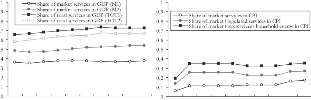
The calculation of the relative price of non-tradables relies on both deflator and CPI price measures. As a first step, the implicit deflators corresponding to the above described productivity series are determined based on nominal and real sectoral GDP. The respective relative prices are calculated subtracting the logarithms of the deflator series of the open sector from those of the closed sector. The same has been done to obtain the relative price of non-tradable goods for the effective foreign benchmark. Finally, the difference between the Estonian and the foreign relative prices is calculated as shown in Table 13. However, it must be noted that the overall GDP deflator and the calculated deflators for the open and the closed sectors do not coincide with the consumer price index. As CPI inflation is at the heart of economic policy in general and of monetary policy in particular, the relative price of non-tradable goods derived from CPI is more appropriate for use instead. We therefore separated the CPI into different goods and service categories. As we have monthly time series of the about 260 items included in the Estonian CPI at our disposal, we could construct series for food, non-food goods, market services, regulated services, household energy, fuel and finally alcohol and tobacco23. Subsequently, we chose to compute two series approximating the development of non-tradable prices. One contains only non-food goods whilst the other also includes food products. It has to be mentioned that the two series behave very similarly as the non-food goods and food series run very closely to each other. The only difference is the higher non-seasonal short-term disturbances in the food series. Next, three series for non-tradable prices are considered. Beside the market service prices, a series including both market and regulated services and a third one containing, in addition, household energy are computed. Based on these data series, we determine six relative price series for Estonia, which are summarised in Table 11.

Table 11. CPI-based relative prices for Estonia

NON-TRADABLES TRADABLES

REL1 MARKET SERVICES NON-FOOD GOODS

REL2 TOTAL SERVICES NON-FOOD GOODS

REL3 TOTAL SERVICES + ENERGY NON-FOOD GOODS

REL4 MARKET SERVICES FOOD + NON-FOOD GOODS

REL5 TOTAL SERVICES FOOD + NON-FOOD GOODS

REL6 TOTAL SERVICES + ENERGY FOOD + NON-FOOD GOODS

For the sake of comparability, the same relative prices have to be used for the foreign countries. For Sweden, we calculate the same series as for Estonia using a 2-digit level disaggregation for CPI prices corresponding to the COICOP. For Finland and Germany, we used 1-digit COICOP data. Finally, we used very disaggregated CPI data (with over 75 categories) for the UK obtained from the Bank of England.

Table 12. CPI-based relative prices for foreign countries

NON-TRADABLES TRADABLES

REL1 MARKET SERVICES NON-FOOD GOODS

REL2 MARKET SERVICES FOOD + NON-FOOD GOODS

REL3 TOTAL SERVICES NON-FOOD GOODS

REL4 TOTAL SERVICES FOOD + NON-FOOD GOODS

23_{For the precise definition of each category, see Appendix. Alcohol and tobacco and fuel are not}

considered in the analysis as they are very often subject to tax changes and to fluctuations in world oil prices.

(20)

Table 13 The difference between CPI-based relative prices in Estonia and foreign countries

ESTONIA BENCHMARK

D_REL1 REL1 REL1

IV. C. The real exchange rate series

The nominal exchange rate series are based on average monthly data in turn based on which of the several real exchange rate series are computed. First, the ones based on the official CPI and industrial PPI indices. Then, the real exchange rate based on goods prices with food and without food is calculated. Finally, a synthetic CPI index based on consumer goods and market services is determined and used for measuring the real exchange rate.

V. A preliminary data analysis

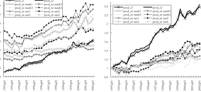
Figure 3 presents labour productivity in absolute values and normalised to the first period for the open sectors, the market-based and the non-market non-tradable goods sectors as described in section four. It can be seen that the level of productivity in the open sector is considerably lower than that in the closed sector, irrespective of whether it is market or market. At the same time, productivity in market non-tradables is still well over that in non-market non-non-tradables. Furthermore, the data also shows that while the rate of growth in the open sector well outpaces that of the closed sector, the market segment of the closed sector clearly lags behind market non-tradables in terms of productivity growth. Hence, the difference between open and closed sector productivities is clearly positive.

Figure 3. Labour productivity in Estonia

10 15 20 25 30 35 40 45 50 19 93q 01 19 93q 04 19 94q 03 19 95q 02 19 96q 01 19 96q 04 19 97q 03 19 98q 02 19 99q 01 19 99q 04 20 00q 03 20 01q 02 20 02q 01 prod_t1 prod_t2 prod_nt mark1 prod_nt mark2 prod_nt mark3 prod_nt mark4 prod_nt nm1 prod_nt nm2 prod_nt nm3 prod_nt nm4 0,8 1 1,2 1,4 1,6 1,8 2 2,2 2,4 19 93q 01 19 93q 04 19 94q 03 19 95q 02 19 96q 01 19 96q 04 19 97q 03 19 98q 02 19 99q 01 19 99q 04 20 00q 03 20 01q 02 20 02q 01 prod_t1 prod_t2 prod_nt mark1 prod_nt mark2 prod_nt mark3 prod_nt mark4 prod_nt nm1 prod_nt nm2 prod_nt nm3 prod_nt nm4

(21)

When constructing the relative price series, the alcohol and tobacco and the fuel items were completely ignored from the CPI because they are all heavily influenced by changes in excise tax and fuel is also subject to changes in oil prices on international markets. Figure 4 below well demonstrates this effect.

Figure 4. Alcohol, tobacco and fuel prices

As to the relative price series, they also show substantial increases over the period under investigation. By using both sectoral deflators and disaggregated CPI data, the price of non-tradables turns out to increase much faster compared with tradable prices. In addition, the market component of tradable prices outpaces market non-tradable prices. This is especially the case for CPI-based measures, as regulated prices grow 2.5 times faster than market service prices.

Figure 5. GDP deflators and CPI

Regulated prices have three major components: public transportation, post and telecommunications and finally rent for publicly owned housing and housing related communal services24. There are at least four main reasons for the huge increases in regulated prices in the past (and possibly the future):

• First, regulated prices were unchanged at the beginning of the transition period when other prices were set free. So, the large increase in regulated prices mirrors a late catch-up with other prices, mainly those of services.

24 In addition, housing energy turns out to be regulated as well as exhibiting one stepwise increase at the beginning of every year. Housing energy is treated separately.

0 0,5 1 1,5 2 2,5 3 3,5 1993 M 01 1993 M 08 1994 M 03 1994 M 10 1995 M 05 1995 M 12 1996 M 07 1997 M 02 1997 M 09 1998 M 04 1998 M 11 1999 M 06 2000 M 01 2000 M 08 2001 M 03 2001 M 10 2002 M 05 fuel&brent 0,96 0,98 1 1,02 1,04 1,06 1,08 1,1 excise Fuel Cruel brent Excise 0,8 1,3 1,8 2,3 2,8 1993 M 01 1993 M 08 1994 M 03 1994 M 10 1995 M 05 1995 M 12 1996 M 07 1997 M 02 1997 M 09 1998 M 04 1998 M 11 1999 M 06 2000 M 01 2000 M 08 2001 M 03 2001 M 10 2002 M 05 alc&tobacco 0,995 1,005 1,015 1,025 1,035 1,045 1,055 excise Alcohol&Tobacco Excise 1 1,5 2 2,5 3 3,5 4 4,5 5 5,5 6 6,5 7 7,5 8 8,5 9 9,5 19 93q 01 19 93q 04 19 94q 03 19 95q 02 19 96q 01 19 96q 04 19 97q 03 19 98q 02 19 99q 01 19 99q 04 20 00q 03 20 01q 02 20 02q 01 defl_t1 defl_t2 defl_nt mark1 defl_nt mark2 defl_nt mark3 defl_nt mark4 defl_nt nm1 defl_nt nm2 defl_nt nm3 defl_nt nm4 1 1,5 2 2,5 3 3,5 4 4,5 5 5,5 6 6,5 7 7,5 8 8,5 9 9,5 19 93q 01 19 93q 04 19 94q 03 19 95q 02 19 96q 01 19 96q 04 19 97q 03 19 98q 02 19 99q 01 19 99q 04 20 00q 03 20 01q 02 20 02q 01 reg_serv nonfood food+nonfood marketserv totserv totserv+energy

(22)

• As soon as the adjustment process has finished, regulated prices are expected to behave similarly and are therefore considered normal market services in the long run. But it is not well known where their target value should adjust to. Furthermore, current prices for regulated services do not yet allow cost recovery, which implies further increases beyond what the B-S effect would imply for normal market services.

• Third, the majority of the regulated sectors are capital intensive. Prices below cost recovery, which do not allow for capital maintenance costs, go in tandem with an ever increasing need for capital investments so as to improve quality and to close the gap on the constantly improving EU standards. Consequently, sooner or later capital investments are to be taken into account.25

• Finally, housing prices in general and thus rents included in the CPI in particular cannot be directly linked to the B-S effect for the following reasons:

a.) Generally, in transition economies, housing prices started adjusting relatively late in the second half of the 1990s: the relative price adjustment of housing turns out to be a slower and longer process than that for other prices26.

b.) This adjustment process accelerates with increasing household incomes and may be accompanied by bubble-like market exuberance. This seems to be also the case in Estonia as shown in Figure 6 below.

c.) Possible tight housing supply could reinforce this.

d.) Non-market rents have undergone a big adjustment process. Even so, they are yet expected to lag behind market rents. Figure 6 also shows that whilst the major hike in rents occurred in 1994–1995, prices for apartments recently started rising sharply, indicating future increases in market rents, and in rents for State-owned housing later on.

25_{This will come either through additional painful price increases or via considerably improved}

efficiency. The former can be achieved by privatisation and market liberalisation. Nonetheless, the scope for the former is very limited due to the difficulty of introducing real competition to, say, the water industry. Efficiency can still be improved under a tight, price cap regulatory regime as the example of the UK has recently shown. (Cf. Saal-Parker, 2000, 2001)

(23)

Figure 6. Regulated rent prices and the price of apartments

Source: Bank of Estonia

Note: The price of apartments refers to those in Tallinn and Tartu, in satisfactory condition: inhabitable, partly in disrepair, no changes to the subdivision, no improvements to the building made, area 54m.

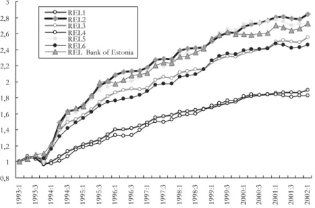
So, as shown in Figure 7 below, the relative price excluding regulated services is substantially lower than the price including them. Comparing these series to the relative price of non-tradable goods using the official non-tradable and tradable series published by the Bank of Estonia, the latter is very similar to those with regulated items excluding household energy.

Figure 7. Relative price measures compared to the official relative price series given by the Bank of Estonia

VI. Are the basic assumptions of the model fulfilled?

There are several assumptions to be verified prior to econometric analysis. The theoretical model explicitly assumes perfect capital mobility between Estonia and the outside world and labour mobility within the Estonian economy. The first assumption is obviously fulfilled with the early implementation of the currency board system: not only are all capital movements liberalised but there are also important de facto capital

0,8 1 1,2 1,4 1,6 1,8 2 2,2 2,4 2,6 2,8 3 19 93 :1 19 93 :3 19 94 :1 19 94 :3 19 95 :1 19 95 :3 19 96 :1 19 96 :3 19 97 :1 19 97 :3 19 98 :1 19 98 :3 19 99 :1 19 99 :3 20 00 :1 20 00 :3 20 01 :1 20 01 :3 20 02 :1 REL1 REL2 REL3 REL4 REL5 REL6

REL Bank of Estonia

1 1,4 1,8 2,2 2,6 3 3,4 3,8 4,2 1 9 9 4 1 9 9 4 1 9 9 5 1 9 9 5 1 9 9 6 1 9 9 6 1 9 9 7 1 9 9 7 1 9 9 8 1 9 9 8 1 9 9 9 1 9 9 9 2 0 0 0 2 0 0 0 2 0 0 1 2 0 0 1 2 0 0 2 Apartment prices Regulated rent

(24)

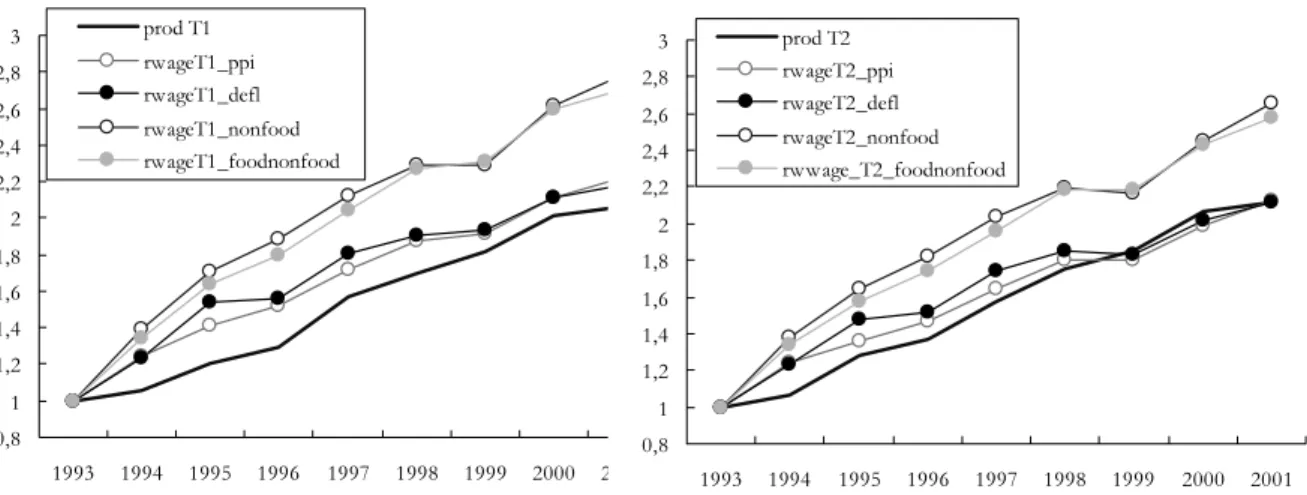
movements to and from Estonia27. As to the labour mobility assumption, it is hard to verify empirically. As it is necessary for the wage equalisation to hold, we have to have a closer look at the wage equalisation process. To begin with we must examine whether the transmission from sectoral productivity growth to the increase in the price of non-tradable goods is secured. As in equation (12) of the model, real wages should be linked to productivity in the open sector. Since we are investigating the model in dynamics, it is most important to check whether changes in real wages deflated by tradable prices are related to productivity developments. Four different tradable price indices – the corresponding sectoral deflator, the PPI, and two CPI sub-indices, namely non-food price inflation and total goods inflation including food – are employed to calculate changes in real wages in the open sector defined as T1 and T228. As can be seen in Figure 8, both productivity measures (PROD_T1 and PROD_T2) move very closely in line with the deflator and the PPI deflated real wage series. Nevertheless, using goods prices from the CPI leads to a different conclusion – even though the short-term dynamics seem to correspond, the real wage measures grow faster and move steadily away from productivity, with a 30% positive gap over the whole period (3,33% a year). Indeed, this is not a serious concern because productivity in the open sector should be in line with real wages when prices in the same sector and not from the CPI are employed.29

Figure 8. Productivity and real wages in the open sector

27_{De facto current account convertibility was achieved in 1992. Full current account convertibility in}

line with article VIII of the IMF and quasi-total capital account convertibility were completed by 1994. Today, the only restriction remaining on capital movements is related to land purchases.

28_{The sectoral nominal wages are weighted using sectoral employment data.}

29_{This means actually that the tradable component of the CPI has risen more slowly than the PPI. This}

can happen because the two indices contain different goods. The PPI consists of domestically produced goods, whereas a large percentage of goods in the CPI are imported goods. It is difficult to say what this share is precisely as CPI statistics do not consider the origins of the goods. As imported goods in household consumption are of importance and because the CPI should broadly reflect household consumption patterns, the share of imported goods should be of a comparable magnitude. Furthermore, there is also a mismatch between the characteristics of the goods included in the two price indices: The PPI contains more industrial goods while the goods component of the CPI includes consumer goods and durable consumer goods. Bearing all this in mind, developments in export and import prices can explain this phenomenon. Export prices have risen compared to import prices, which in turn means that the PPI including a great deal of exported goods has experienced greater increases than the goods component of the CPI which contains a considerable amount of imported goods.

0,8 1 1,2 1,4 1,6 1,8 2 2,2 2,4 2,6 2,8 3 1993 1994 1995 1996 1997 1998 1999 2000 2001 prod T1 rwageT1_ppi rwageT1_defl rwageT1_nonfood rwageT1_foodnonfood 0,8 1 1,2 1,4 1,6 1,8 2 2,2 2,4 2,6 2,8 3 1993 1994 1995 1996 1997 1998 1999 2000 2001 prod T2 rwageT2_ppi rwageT2_defl rwageT2_nonfood rwwage_T2_foodnonfood

(25)

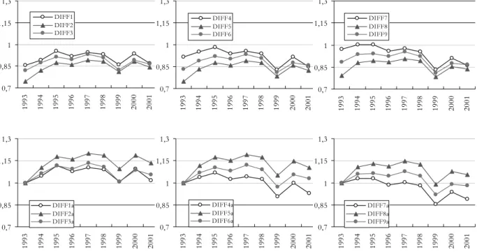
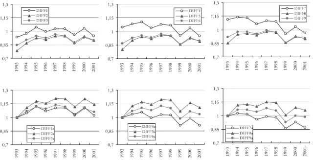
The second step is to find the extent to which nominal wages equalise between the open and the closed sectors30. Nominal wages in the open sector seem to be lower than those in both the market-based closed sector including transport and communication and the closed sector as a whole (see Figure 9) – independently of whether or not construction is considered. The absolute wage equalisation may be slightly better achieved between the open sector and the market-based closed sector including transport and communication as the ratio is closer to unity. However, looking at relative figures shows, seemingly paradoxically, that the wage ratio may follow a downward trend whereas in the two former cases, the ratio turns out to be rather stable.

Figure 9. The wage equalisation process in absolute and relative terms, 1993– 2001

The analysis of the individual sectors reveals that this is mainly due to huge wage increases in financial intermediation. While wages in other sectors move in line over the period considered, wages in financial intermediation, already initially higher, show by far the fastest growth.

30_{The open and closed sectors are defined as for the productivity and the deflator, and the equalisation}

is considered for the differences developed for productivity, that is, DIFF1 to DIFF9 where data for the open sector is divided by that for the closed sector.

0,7 0,85 1 1,15 1,3 19 93 19 94 19 95 19 96 19 97 19 98 19 99 20 00 20 01 DIFF1 DIFF2 DIFF3 0,7 0,85 1 1,15 1,3 1993 1994 1995 1996 1997 1998 1999 2000 2001 DIFF4 DIFF5 DIFF6 0,7 0,85 1 1,15 1,3 1993 1994 1995 1996 1997 1998 1999 2000 2001 DIFF7 DIFF8 DIFF9 0,7 0,85 1 1,15 1,3 1993 1994 1995 1996 1997 1998 1999 2000 2001 DIFF1a DIFF2a DIFF3a 0,7 0,85 1 1,15 1,3 1993 1994 1995 1996 1997 1998 1999 2000 2001 DIFF4a DIFF5a DIFF6a 0,7 0,85 1 1,15 1,3 1993 1994 1995 1996 1997 1998 1999 2000 2001 DIFF7a DIFF8a DIFF9a

(26)

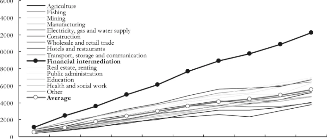
Figure 10. Average nominal wages in 15 sectors in Estonia, 1993-2001 (EEK)

By eliminating wages in financial intermediation from the closed sector, the ratio turns out to be very close to unity. In addition, if transport and telecommunications are taken as a market-based non-traded goods sector, the ratio proves to be more stable than if they are excluded. So, it is not false to state that wages seem to be ready to transmit the effect of productivity growth onto non-tradable prices. However, given the institutional setting in Estonia, it remains somewhat unclear how wage equalisation comes about. First, labour mobility across sectors is rather unidirectional in Estonia. If the open sector is the leader in wage setting, and if wages grow faster there, mobility towards the open sector should be observed. In practice, the opposite has happened in Estonia. Over the last 10 years, the number of employees has dramatically decreased in the open sector while it has slightly increased in the market-based non-traded goods sector31. Second, given that union density in Estonia is one of the lowest among transition economies32 and because unions are present mainly in mining and the public sector, trade unions cannot promote the equalisation of wages across the whole economy.

31_{The difference is apparently absorbed by the decreased activity rate.} 32_{See Paas et al. (2002), pp. 55.}

0 2000 4000 6000 8000 10000 12000 14000 16000 1992 1993 1994 1995 1996 1997 1998 1999 2000 2001 Agriculture Fishing Mining Manufacturing

Electricity, gas and water supply Construction

Wholesale and retail trade Hotels and restaurants

Transport, storage and communication Financial intermediation Real estate, renting Public administration Education

Health and social work Other