Productivity and Tradability

Preliminary and incomplete. Please do not quote.

Comments welcome

Productivity and Tradability

Paul R. Bergin

University of California at Davis and NBER Reuven Glick

Federal Reserve Bank of San Francisco This draft: November 30, 2003

Abstract:

This paper shows how heterogeneity in trade costs and heterogeneity in productivities work together to determine features of the international trade pattern. This is demonstrated in a general equilibrium macroeconomic model, where a convenient methodology is developed for allowing the status of a good as traded or nontraded to be determined endogenous ly. While the two sources of heterogeneity are found to be interchangeable in determining the relative tradability of goods, they have very different implications for relative prices, such as the real exchange rate. The interaction of these two factors is found to be important for understanding the Balassa-Samuelson effect, in which richer countries tend to have more appreciated real exchange rates. This effect will tend to be stronger the more negatively related are trade costs and productivity distributions. Further, the magnitude of the Balassa-Samuelson effect is found in simulations to double when one allows the distinction between traded and nontraded goods to evolve endogenously in response to heterogeneous productivity shocks.

JEL classification: F4

_______________________

The views expressed below do not represent those of the Federal Reserve Bank of San Francisco or the Board of Governors of the Federal Reserve System.

P. Bergin, Department of Economics, University of California at Davis, One Shields Ave., Davis, CA 95616 USA [email protected], ph (530) 752-8398, fax (530) 752-9382.

R. Glick, Economic Research Department, Federal Reserve Bank of San Francisco, 101 Market Street, San Francisco, CA 94105 USA [email protected], ph (415) 974-3184, fax (415) 974-2168.

1. Introduction

This paper shows how heterogeneity in trade costs may work together with heterogeneity in productivities across goods to jointly determine features of the pattern of international trade. It then goes on to show that the macroeconomic implications of technology shocks change, once one views the trade pattern as endogenous.

Open economy macroeconomics has made significant advances in the last decade, particularly in terms of grounding models of the macroeconomy in microeconomic foundations. However, it has tended to take as exogenously given important aspects of the pattern of

international trade. In particular, many open economy macro models rely on the fact that some goods produced domestically are not traded internationally; this dichotomy between traded and nontraded goods has been foundational to several key results in open economy macroeconomics. Yet the demarcation between traded and nontraded sectors of the economy in these models is typically taken as given, with nontradedness assumed to be an inherent feature of some goods.

A prominent example is the theory of Balassa (1964) and Samuelson (1964), which aims to explain the long-run behavior of the real exchange rate. In particular, it offers an explanation for why rich countries tend to have appreciated real exchange rates. Their explanation lies in supposing that technology improvements disproportionately affect the tradable goods sector. Our analysis suggests that technology developments themselves may well alter the trade pattern on which the Balassa-Samuelson theorem depends.

Unlike open economy macro, trade theory has long studied the endogenous development of trade patterns. Beginning with Dornbusch, Fisher, and Samuelson (1977), there has been an interest in seeing how the goods along a continuum that are exported or imported are determined endogenously, with a range of goods possibly remaining untraded due to trade costs. Recent work has proposed clever ways of parameterizing the firm heterogeneity that is necessary for an equilibrium trade pattern. But in all this work, goods are ranked by their productivities, while the magnitude of trade costs is assumed to be uniform across goods. Those goods with the greatest comparative advantage in one country or the other are traded, while those goods with small gains from trading relative to the uniform trade costs remain nontraded.

However, since some goods are much more difficult to trade than others, the identity of a good as traded or nontraded is likely to be determined by heterogeneity in trade costs as well as by comparative advantage based on productivity. For example, the reason that many types of services are nontraded is not because countries are so similar in their productivities in these sectors; rather, they remain nontraded primarily because such services are particularly difficult to trade over long distances.

Empirical work by Hummels (1999, 2001) has emphasized that trade costs -- including tariff and nontariff barriers, shipping costs, and other associated costs of marketing and

distribution -- vary greatly across classes of goods and play an important role in trade decisions. Collecting detailed trade data for individual goods, he finds that freight costs alone can range from more than 30 percent of value for raw materials and mineral fuels down to 4 percent for some manufactures. Depending on factors such as weight, distance, and the time sensitivity of demand, trade costs can be high and variable for many manufactured goods as well. Hummels (2001) documents that in 1998 a substantial proportion of U.S. trade was airshipped with air-freight costs typically amounting to 25 percent of transported good value in some cases.1 _{In a} broad survey of trade cost evidence, Van Wincoop and Anderson (2003) likewise reach the conclusion that trade costs are very large and very heterogeneous among goods.

Empirical work has also found support for the idea that some goods do switch over time between status as traded and nontraded. Using a panel of U.S. manufacturing plants from 1987 to 1997, Bernard and Jensen (2001) find that year to year transition rates are noteworthy: on average 13.9% of non-exporters begin to export in any given year during the sample, and 12.6% of exporters stop. It should be noted that the results of this paper in no way rely upon impla usibly large numbers of firms switching between traded and nontraded status, but rather upon the simple fact that firms have the ability to make such a switch.

This paper develops a macroeconomic model to study how heterogeneity in both productivity and trade costs interact to determine which goods are traded. The model includes

1 _{Even these measured trade cost margins may be severely biased downwards. Average transportation cost} measures that weight costs of individual goods by the value of observed trade flows underestimate costs to the extent that goods with higher costs are traded less. Second, if vertical production arrangements imply transshipment of raw materials and intermediate goods, the cumulative transportation costs can be much higher than those on the exports of the final product alone.

two countries, each of which produces a distinct continuum of varieties. These goods are

heterogeneous in terms of the technology in their respective production functions and the iceberg costs they incur in international trade. We posit convenient distributions for technology and for iceberg costs, which permit us to aggregate over the heterogeneous goods, and evaluate aggregate prices and quantities in this macroeconomy. Firms are assumed to be monopolistically

competitive. The only factor of production is labor, with no physical capital. The model environment is limited to balanced trade in goods, with no trade in assets.

What distinguishes the model from standard open economy macro models is that it views traded and nontradeds not as separate types of goods, but instead as two regions along a single continuum of goods, where the dividing point along this continuum is determined endogenously. While many recent open economy macro models are built upon a continuum of goods, these have assumed all goods within a group are identical. This model takes heterogeneity seriously, and by finding a simple way of dealing with it, permits us to examine how classic results in the field change when one alters the degree of heterogeneity and the underlying distinction between tradeds and nontradeds. Operationally, this is made possible by specifying a convenient

distribution of the heterogeneous factors which is easy to aggregate over, and by taking the share of nontraded goods as an endogenous variable rather than as a fixed parameter. An equilibrium condition is derived for this new variable, which describes whether a firm will generate extra profits by selling its good abroad, after accounting for iceberg and fixed costs of trade.

This simple framework is sufficient to shed useful light on the interactions between productivity and trade costs in determining which goods are traded. Because both affect the marginal costs of goods sold abroad, they enter the decision of whether to export in an identical manner; it is the net effect of the two that determines the traded status of that good. A good that is especially costly to trade may be traded nonetheless, if the productivity of that good relative to other potentially tradable goods is sufficiently high to compensate for the extra trade cost. Conversely , even if a good has a high level of productivity, if it has very large trade costs, it may not be traded, while goods with lower productivity may be traded, due to lower trade costs. A rise in the heterogeneity between goods in either of these two dimensions will tend to raise the share of nontraded goods in an economy. This is because the marginal exporter compares his

relative price and level of demand for his export in the foreign market. A rise in heterogeneity along the continuum of goods will increase the average level among exporters relative to that of the marginal exporter, causing the marginal firm to exit the export market.

However, these two dimensions of heterogeneity are not identical in all respects, as trade costs affect prices differently in foreign compared to domestic markets. So unlike productivity heterogeneity which affects pricing in domestic and foreign markets equally under standard monopolistic competition price setting, only trade costs can create the type of heterogeneous pricing to market and the deviations from the law of one price that we observe in data. Further, because trade costs and productivity affect relative prices differently, these two sources of heterogeneity are found to have extremely different implications for real exchange rate behavior and the Balassa-Samuelson theorem. This result differs from the marginal export decision underlying a good’s tradedness, because the real exchange rate depends on the relative

productivity of exports net of transport costs compared to the relative productivity of all goods sold at home, where the latter is not affected by transport costs. Consequently, while a rise in heterogeneity in terms of productivities will tend to generate a real exchange rate appreciation, greater heterogeneity in trade costs will imply counteracting effects on the real exchange rate. Our framework also provides a generalized version of the Balassa-Samuelson theorem with several interesting implications. Since the productivities of individual goods differ along a continuum goods, the distribution of technology improvements must be sufficiently biased toward goods with low trade costs for the real exchange rate to appreciate. So the Balassa-Samuelson theorem becomes a matter of degree, and our model makes clear what determines this threshold value. Second, the magnitude of the Balassa-Samuelson effect in our model depends upon the degree of heterogeneity in trade costs – if one changes the degree of the underlying distinction between traded and nontraded goods , then a given productivity increase will have different effects on the real exchange rate. Thirdly, the model shows that allowing the trade pattern to evolve endogenously in response to productivity shocks alters the nature of Balassa-Samuelson effects. For example, allowing the share of nontraded goods to rise endogenously in response to a biased productivity gain tends to double the size of the effect on the real exchange rate. Finally, our model suggests that the degree of Balassa-Samuelson effects can wax and wane over time, as the

two factors determining the trade pattern – productivity and trade cost heterogeneity – compete against each other and as one grows over time to dominate the other.

Our analysis is related to several other recent papers in the literature. Obstfeld and Rogoff (2000) demonstrated that introducing trade costs into simple macro models can have dramatic implications for understanding a range of open economy issues, Betts and Kehoe (2001a,b) developed a full-scale macro model with trade costs. This mode l differs from ours in that it does not have a range of goods that are fully nontraded. Ghironi and Melitz (2003) develop a macro model in which goods can switch between traded and nontraded; further their model allows for entry and exit from production, which our model does not permit. But another difference is that their model allows heterogeneity only in the dimension of productivities, whereas our focus is on the role of heterogeneity in trade costs and how this interacts with productivity differences.

2. Model

Consider a model of two countries, Home and Foreign, in which each country completely specializes in production of a distinct differentiated good. In each country there is a separate continuum of firms each producing a different variety of the local differentia ted good, denoted by H and F, respectively. All goods produced in each country have the potential to be exported, but some endogenously determined fraction will be nontraded in equilibrium. Quantities and prevailing prices for the H or F goods consumed in the foreign country are denoted by *. In the following we specify the model equations for the Home country; the counterpart equations for the foreign country are for the most part relegated to an appendix.

Consumption

*

,

C C is the level of aggregate consumption by home and foreign agents, respectively, defined as a CES aggregate of consumption of each country’s own goods (CHin the home country, *

F

C in the foreign country) and imports of the other country’s traded (export) goods

( _, *

FT HT

( )

(

)

1 ₁ 1 _{1 1} (1 ) H FT C C C γ γ γ γ γ _γ γ _γ θ − θ − −   =_ + − _   (1)

( )

( )

1 1 1 1 1 * * _{(1 )} * F HT C C C γ γ γ γ γ γ γ γ θ − θ − −   =_ + − _   (1*)

where γ is the elasticity of substitution between domestic and foreign goods and θ is an own-goods bias coefficient.

The continuum of goods produced in each country is indexed by i on the interval

[ ]

0,1 .2 Let n and _n* _{denote the (endogenous) share of these in each country that are nontraded, where}

goods are ordered such that

[ ]

0,n and

[

_0,n*

]

_{are nontraded and}

[ ]

_{n,1 and}

[ ]

_n*_{,1 are traded.}

Accordingly, home country consumption of its own-produced good (CH ) is defined as a CES index of nontraded (CHN) and traded (CHT) home goods:

( )

( )

( )

(

)

1 1 1 1 0 1 1 1 1 n H Hi Hi n HN HT C c c di C C n n n n φ φ φ φ φ φ φ φ φ φ − − − − − = +     = _{  + −  } −    

∫

∫

(2) where

( )

1 ₁ 1 0 1 n HN Hi C c di n φ φ φ φ φ − − _{ }    ≡  _{  } 

∫

 ,

( )

1 ₁ 1 1 1 1 HT Hi n C c di n φ φ φ φ φ − − _{ }    ≡ _{ −} _{ } 

∫

 (3)

Lower case c is used to denote consumption of individual varieties i of each differentiated good and φ is the elasticity of substitution between varieties.3 _{Analogously, the consumption indices} of the foreign good imported by home residents C_{F T} is defined as

( )

* 1 ₁ 1 1 * 1 1 FT Fi n C c di n φ φ φ φ φ − − _{ }    ≡ _{ −} _{ } 

∫

 (4)

2 _{Note that, although each country produces a distinct set of goods, in our notation we use the same index i} to order goods along each continuum. We assume that the mass of firms is the same (1) in each country and do not allow entry of new firms into production, as in Ghironi and Melitz (2003) Relaxing these

assumptions are possible extensions in future research. 3 _{That is, /}

(

_/

)

Hi cHj pHi pHj

Foreign country consumption of its own-produced good * F C , nontraded ( * FN C ) and traded ( * F T C ) foreign goods, and consumption of the traded home good that is imported by foreign residents ( *

HT

C ) are defined analogously (see the appendix). Note that the ela sticity of substitution is assumed constant across countries.

Prices and relative demands

Price indexes are defined as usual for each category of goods, in correspondence to the consumption indexes above. For the Home country, the aggregate price level P is an index of the prices of home goods PH and of imported foreign goods PFT

( )

( )

(

)

1 1 1 1 (1 ) H FT P_≡ θ P −γ _{+ −}θ P −γ −γ (5) where the home goods price is in turn an index of the prices of nontraded home goods

HN

P and of nontraded home goods PHT

( )

( )

( )

( )

1 1 1 1 0 1 _{(1 )} 1 n H Hi Hi n HN H T P p di p di n P n P φ φ φ φ φ − − − − − = + = + −

∫

∫

₍₆₎ and 1 1 1 0 1 n HN Hi P p di n φ φ − − _{ }  ≡  _{ }  

∫

 , 1 1 ₁ 1 1 1 HT Hi n P p di n φ φ − − _{ }  ≡ _{ −} _  

∫

 (7)

while the domestic price (to Home residents) of the imported traded foreign good is given by

* 1 1 1 1 * 1 1 FT Fi n P p di n φ φ − − _{ }  ≡ __{ −} _ _ 

∫

 (8)

The consumption and price indices imply the following relative demand functions for domestic residents over aggregate home and foreign-produced output:4

(

)

/ /

H H

C C=θ P P −γ, C_FT/C= −(1 θ)

(

P_FT/P

)

−γ (9) and over nontraded and traded home goods output

4 _{Also note that the CES specification implies for individual goods variety i : /}

(

_/

)

Hi H H i H

c C = p P −φ

( )

1

(

)

(

)

1

(

)

/ / , / 1 /

(

)

/ /

HN H HN H

C C =n P P −φ, C_HT /C_H = −

(

1 n P

)(

_HT /P_H

)

−φ (10) Production, productivity, and transport costs

The production sector in each country consists of constant-returns-to-scale technologies for the output of each differentiated good. For the Home country:

H i i H i

y =Al (11)

where yHi represent the level of output, l_Hidenote workers employed in production, and Ai are productivity coefficients for each individual good i. We employ the usual assumption that labor is mobile across sectors within each economy, but immobile across countries.

Profit maximization under monopolistic competition implies pricing is determined by the standard cost markup rule. For domestic sales of all home goods, either traded or nontraded goods [0,1] 1 Hi i W p i A φ φ = ∈ − (12)

where

W

denotes the home wage rate, and for export sales of traded goods

* 1 _{[ ,1]} 1 1 Hi i i W p i n A φ φ τ = ∈ − − (13)

where τi is the fraction of each good i lost during shipment and it is assumed that foreign residents fully absorb the cost of shipping.5 _{Thus for each traded good the domestic and foreign} sales price differs by the proportion1/ 1

(

−τ_i

)

:

* 1 1 Hi Hi i p p τ = −

Note that, in the absence of transport costs, sales prices are equalized across markets for each good i, i.e. * _, *

Hi Hi Fi Fi

p =p p = p .

We assume that transport cost differences across goods are monotonically declining in i, as specified by the following functional forms:

5 _{For example, if 0.5}

i

τ = , then 50% of good i is lost in shipment and the firm doubles the price of the good that reaches the foreign market.

(

)

1− =τ α_{i τ} 1+λi βτ , 1>α_τ >0;λ β, _τ >0 (14) The parameter α_τ controls the level of the distribution, while

λ

and β_τ control the rate at which transport costs fall with i. An increase in α_τ represents a balanced increase in transport costs that affects all goods equally. An increase in

λ

biases transport cost declines towards goods with higher i indices. A higher β_τ increases the rate at which costs fall for a given percent change in the index. The restriction 1>α_τ ensures that in the absence of trade cost heterogeneity, i.e. β_τ =0, there are still positive iceberg costs for all goods, i.e. τi = −1 ατ >0 for all i.

We assume that the variation of productivity across firms follows the same functional form:

(

1

)

A, , 0

i A A

A=α +λi β α λ > (15)

Changes in αA,

λ

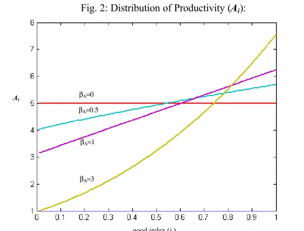
, βA have effects on the distribution of productivity similar to their analogues for transport costs. Higher α_A represents a balanced productivity improvement that affects all goods equally. An increase in

λ

biases productivity increases towards goods with higher i

indices. The magnitude of β_A affects the curvature of the productivity distribution and hence the degree of heterogeneity across goods. A higher βA increases the rate at which productivity changes for a given percent change in the index. The sign of β_A affects the ordering of productivity differences. In the discussion below we generally assume that productivity is ordered in the same way as transport cost, i.e. β_τ >0 and βA >0 and hence transport costs fall and productivity rises with i. However, where appropriate we consider the case where they are ordered in opposite directions, i.e. β_τ >0 and βA<0 and productivity declines with i.

Our specification of the distribution of productivity levels implies the average (weighted) productivity level at home A% (the analogue for the foreign country is denoted _A%*_{) can be defined}

as6

[

]

(

)

1 1 ₁

( ) (

₁

)

0 1 1 , A A A i A A A A di ω φ _{φ φ} λ α ω α λω − _{− −} + − ≡

_∫

= % ₍₁₆₎

An increase in αA or ωA raises the economy-wide average productivity.

7 _{Note, however, that}

A% is independent of n and hence do not depend on the nontraded vs. traded goods composition of the economy.

Given the cutoff between nontraded and traded goods at index n, it is straightforward to compute the price index for nontraded home goods by using (12) and (15) to substitute for pHi in (7)

(

)

1 1 1 0 1 1 1 1 1 1 1 A n HN i A A W P di n A n W n φ φ ω _φ φ φ λ φ φ α λω − − − _{ } _{ }     = _{   }   _ −  _    _{+ −}      = _{  } −   

∫

(17)

where ω_A≡ −1 β_A(1−φ) 1> if β_A≥0 since φ>1. Analogously substituting into (7) gives the price index of traded home goods:

(

) (

)

(

)

1 1 1 1 1 1 1 1 1 1 1 1 1 A A HT i n A A W P di n A n W n φ φ ω ω _φ φ φ λ λ φ φ α λω − − − _{ } _{ }     = _{   }  −  _ −  _    _{+ − +}    =_{ }   −  −    _{ }

∫

(18)

Equations (17) and (18) express the prices of nontraded and traded goods as functions of the share of nontraded goods n, the elasticity of substitution across goods φ, the wage rate W, and the

6 _{As pointed out by Melitz (2003), weighting by the elasticity parameterφ, makes the weights proportional} to the relative output shares of firms.

7 _Formally, %

₍

₎

( )

(

)

[

]

(

)

(

)

(

)

2 1 1 1 / 1 ln 1 1 0 1 if ln 1 1 if 1 1 1. A A A A A A A A A A A A ω ω ω ω ω λ ω ω λ λ ω λω _{λ ω} λ λ λ ω + − ∂ _{∝ ∂ ∂ = + − + + >} ∂ + > − +    _{ } +     _{  }         >  

productivity parameters, αA, βA, and λ. Keep in mind that n is itself an endogenous variable that will be solved as part of the general equilibrium system.8

Defining the average level of productivity in production of the nontraded and traded home goods (where the notation indicates that each is an implicit function of the endogenous n, as well as the other parameter arguments αA, ωA)

9_:

[

]

(

)

1

( )

₁

( ) (

₁

)

0 1 1 1 ; , A n N A A i A A n A n A di n n ω φ _{φ φ} λ α ω α λω − _{− −} + − ≡

_∫

= % ₍₁₉₎

[

]

(

)

1 1 1 ₁

( ) (

₁ 1

)

(

1

)

; , 1 (1 ) A A T A A i A A n n A n A di n n ω ω φ _{φ φ} λ λ α ω α λω −   _{− −} + − + ≡_{ } = − −  

∫

% ₍₂₀₎

Taking first derivatives of (20) establishes the property that, if productivity rises with the index i

(βA>0 ) and henceωA>1, ∂AT/∂ >n 0, i.e. average productivity rises in the traded sector with increasing n.10 _{Intuitively, as the share of nontraded goods in the economy rises, goods at the} low productivity end of the traded goods sector become nontraded, and the average level of productivity of all remaining traded goods rises. These effects are reversed if ωA<1; i.e. an increase in n then is associated with lower average productivity in the traded goods sector.

With (19) and (20), we may rewrite (17) and (18) as (where the dependence on the exogenous productivity parameters is suppressed in the notation):

[ ]

1 HN N A W P n φ φ = − % (21)

8 _{Note that (17) is well-defined and positive for 0}

A

ω < as well as forω_A>0 since the numerator and denominator always have the same sign; the same is true for all productivity and price aggregates defined elsewhere in our analysis.

9 _Note

( )

1

(

[ ]

)

1

(

[ ]

)

1 (1 ) N T A% φ− =n A n% φ− + −n A n% φ− _{. It is straightforward to demonstrate}

[ ]

(

)

(

1

)

(1 n A n) _T φ− / n 0 ∂ − % ∂ < _. 10 _{Formally, since}

[ ]

_{[ ]}

(

1

)

(

1

)

(1 ) A A A T n n Z n n A ω ω λ λ λω + − + ∝ ≡ −

% _{, it can be shown that} AT ₀

n ∂ _>< ∂ as

(

)

(

)

(

)

(

)

1 2 2 1 1 1 1 1 (1 ) 1 0 (1 ) (1 ) (1 ) 1 1 A A A A A A A A A n n Z n n n n n n n ω ω ω ω λ λ ω λ λ λ ω λ λω λω λω λ λ − + − + + ∂ _{= − =} + _{− −} − _> < ∂ − − − + + _{ }  _ _   

[ ]

1 HT T W P A n φ φ = − % (22)

In this form we see that prices are markups of the average marginal cost -- wage over average productivity -- in each sector.

Substituting for P_HN,P_HT with (21) and (22), respectively, in expression (6) gives

(

)

_° 1 1 1 1 1 1 1 1 A H A A W P W A φ ω φ _λ φ φ α λω φ −      _{ } = _{   } + − _ = − _{    } − (23)

Thus the aggregate price of home goods depends on wages

W

and average aggregate productivity A%. Since A%is independent of trade costs and n, these variables affect PH only through their effects on the average wage level in the economy.

The foreign price (to Foreign residents) of the home good exported abroad is

(

) (

)

(

)

1 1 ₁ 1 * 1 1 1 1 1 1 1 1 1 1 1 HT i i n A W P di n A n W n φ φ ω ω _φ τ φ φ τ λ λ φ φ α α λω − − − _{ } _{ }     = _{   }  −  _ − −  _    _{+ − +}    =_{ }   −  −    _{ }

∫

(24)

where ω≡ −1

(

β_A+β_τ

)

(1−φ). We define the “effective” productivity of home good exports as

[ ]

(

1

)

X i i

A i =A −τ , i.e. productivity adjusted by the transport costs of goods exported abroad, since higher τ effectively lowers the productivity of these goods relative to the same goods sold domestically. Note that β_A+β_τ >0 implies A i_X′

[ ]

>0, i.e. effective productivity of export goods rises with higher i. However, forβ_τ >0, if productivity declines with i (βA<0) sufficiently to make βA+βτ <0, effective productivity may decline.

The average effective productivity of home good exports A%X is defined by

(

)

₁ 1

( )

(

)

(

) (

)

1 1 1 1 1 ; , , 1 (1 ) X A Xi A n n A n A di n n ω ω φ φ φ τ τ λ λ α α ω α α λω −   − − + − +   ≡_{ } =   _{ − }

∫

₋ % ₍₂₅₎ as ωA >< 1.

As with the case ofA%_T, the effect of n on A%_Xdepends on whether or not the parameter ω>1, which in turn depends on the transport and productivity curvature parameters β βA, τ . A sufficient condition for ω>1 and ∂A%_X/∂ >n 0 _{is 0}

A τ

β +β > , i.e. effective productivity of exports rises with the index i. Note that, even if the ordering of transport costs and productivity across goods are reversed (βA<0,βτ >0), the sum βA +βτis still positive and ω>1as long asβτ > −βA>0.

Substituting (25) into (24) implies that the price of home country exports may be

expressed (where we again suppress the dependence on the exogenous productivity parameters in the notation) as

[ ]

* 1 HT X W P A n φ φ = − % (26)

Comparison of (20) and (22) with (25) and (26) indicates that in the presence of transport costs X T

A% <A% _{, implying} *

HT HT

P <P , i.e. the price to foreign residents of exported home goods is higher than the domestic price of the same goods at home. It should be noted that as long as transport costs vary across goods, the difference between A%X and A%T and hence

*

and HT HT

P P is not

constant and depends on n. In the special case of no trade cost heterogeneity (β_τ =0), however, A

ω ω= and *

HT HT

P =α_τP , i.e. aggregate domestic prices of traded goods are less than export sales by the constant factor α<1. In the absence of any transport costs at all, all goods are traded (n=0), implying A A% = %X =A%T, and

*

H HT HT

P = P = P . Marginal trading condition

To help pin down the equilibrium share of nontraded goods note that at the margin the producers of the borderline nontraded--nontraded good must be indifferent between home and foreign sales. That is, the (real) operating profits from exporting the nth home good must equal the (real) fixed cost of exporting f_X:

* 1 1 * 1 Hn Hn X n i W W p c f A τ P P  ₋   ₌   ₋  _{ }  _{ }   (27)

where the operating profits are defined as the export price minus marginal cost times the volume of sales to foreign residents. Note that real operating profits are expressed in terms of the price of the domestic consumption basket P. We follow Ghironi and Melitz (2003) in assuming that firms employ domestic workers to cover the fixed costs. With f_X measured in units of effective

domestic labor, we define W P/ as the effective real wage rate of this labor and express these labor costs as

(

W P f/

)

_X.11

Since the condition * _/ *

(

₁

)

1

(

* _/ *

)

Hi HT Hi HT

c C = −n − p P −φ holds for all goods i in the range [ ,1]n , it can be used to substitute for *

Hn

c , so (after canceling the variable P from both sides) * * * * 1 1 1 1 Hn Hn HT X n i HT p W p C Wf A n P φ τ −  _{ }  − =  ₋ _{ −} _     Substituting for * Hn

p with (14) and (17), defining A n_X

[ ]

≡A_n

(

1−τ_n

)

(

1

)

A

A n τ β β τ α α λ + = + as the

effective productivity of exports of the nth good, multiplying and dividing by *

HT

P , and substituting with (24) for *

HT

P in the denominator on the lefthand side gives

[ ]

[ ]

1 * * 1 1 1 X HT HT X X A A n P C Wf n n φ φ − _{    } _{    } = − _{  }    %  (28)

Observe that export profits depend on the effective productivity of the nth good ,A n_X

[ ]

, relative to the average of all exported goods, A n%_X

[ ]

. For given aggregate export sales * *

HT HT

P C , when no goods are traded (n=1), the marginal profitability of exporting is very high. As long as profits exceed the fixed costs of exporting, more goods will become traded and n declines. As n falls, the relative productivity and profitability of the marginal exported good declines; in equilibrium

11 _{In general, the effective labor employed to cover the fixed costs should depend on the productivity of the} labor employed and the real wage rate should be scaled by this level of productivity, which we can

denoteA_fX. A_fXmay be assumed exogenously given or related to productivity elsewhere in the economy, e.g. %A, the average aggregate productivity level. We abstract from this issue by normalizing A_fXto 1.

profits are reduced to just covering the fixed costs of the nth good entering into the foreign export market. 12

Labor market equilibrium

Labor market equilibrium in the domestic country requires that labor employed in production of nontraded and traded home goods plus labor employed to cover the fixed costs of exporting equal the (exogenous) domestic labor supplyLH

13_: 1 0 (1 ) n Hi Hi X H n l di + l di + −n f =L

∫

∫

(29)

Substituting for l_Hiwith the production function (11):

1 0 * 1 0 (1 ) 1 (1 ) n Hi Hi X H i n i Hi Hi n Hi i X H i n i y y d i d i n f L A A c c c d i d i n f L A A τ + + − = + − + + − =

∫

∫

∫

∫

since * y , [0, ] y [ ,1] 1 Hi Hi Hi Hi Hi i c i n c c i n τ = ∈ = + ∈ −

Substituting with c_Hi/C_H =

(

p_Hi/P_H

)

−φ and * _/ *

(

₁

)

1

(

* _/ *

)

Hi HT Hi HT c C = −n − p P −φ gives 1 * * * 0 1 1 1 (1 ) 1 1 n Hi Hi Hi H H HT X H i H n i H i HT p p p C di C C di n f L A P A P n P φ φ φ τ − _ − − _     _   _{ }   _ + _{ } + + − =   _   ₋ _{ −} _   _    _{ }     _

∫

∫

12 _{This can be shown formally by defining per unit export profits}

[ ]

(

[ ]

)

[ ]

(

)

(

(

(

)

)

)

1 1 1 1 1 1 0 (1 ) 1 (1 ) X X A n n X n n n A n φ ω φ ω ω λω λ φ φ λ λ − − − + ≡ = > + − + −        

  %   and noting that

[ ]

₍

₎

[ ]

0 1 1 lim lim , / 0 (1 ) 1 n X n ω n X n X n λω φ λ → = + − < → = ∞ ∂ ∂ >      

13 _{When all home goods are nontraded, i.e. n = 1, then no labor is employed to cover fixed costs of} exporting.

Using (14) and (17) in turn to substitute for _, *

Hi Hi

p p and evaluating gives the following expression for the domestic wage as a function of domestic and foreign demand for the home good as well as the nontraded goods share and the productivity parameters:

(

)

( )

( ) ( )

_{( )}

(

) ( ) (

(

)

)

1/ 1 * * 1 1 1 _* 1 1 (1 ) 1 1 1 1 1 A H X H H HT HT A A A H HT W L n f n P C P C n P P φ φ ω ω ω φ φ φ φ τ φ φ λ λ λ α α α λω λω − − − − −  −  = − − _{ }⋅   _{   + − }   _{ + − + } _{   +}  _{ }       _{   }   _{ − }      

Substituting next with (16) and (25) for the definitions of A A n%, %_X

[ ]

(

)

_{( )}

( )

( )

( )

1 * * 1 1 1/ 1 _* 1 1 (1 ) H H HT HT H X X H HT P C P C W L n f A A P P φ φ φ φ φ φ φ φ − − − − − _{ }     _{− } _{  }   = − − _{   } +_{  }  _{  } % _{ } % _ Substituting for _, * H HT

P P with (6), (24) and canceling terms gives

(

)

( )

[ ]

[ ]

(

)

(

)

1 * * 1 1 1/ 1 1 1 * * 1 (1 ) 1 1 1 (1 ) H H HT HT H X X X H X H H HT HT P C P C W L n f A A n W _W A A n L n f P C P C φ φ φ φ φ φ φ φ _{φ φ} φ φ φ φ − − − − − − _{ }    _{ }         −    = − −  _{ } _ +        _{ }        _{ − } _ _{ − } _          _{− } _ = − − _{ } + _   % % % % (30) or * * 1 (1 ) H X H H HT HT WL n f W φ P C P C φ  _{− } _ − − =_{ } + _  

i.e. the domestic wage bill -- net of wages paid for workers employed in covering fixed costs, (1 ) _X

W −n f -- is proportional to the value of home goods consumed domestically or exported, with the proportionality constant equal to 1 minus the profit rate 1/φ.

Closing the model

We close the model with the balanced trade condition that the value of exports equals the value of imports

* *

HT HT FT FT

and the normalization condition14

* ₁

P = (32)

Equilibrium determines the 24 variables ,C C_H,C_HN,C_HT,C_FT P P P, _H, _HN,P_HT,P_FT,W , and

n

and their foreign counterparts (denoted by *) by solving the system of 24 equations (1), (2), (3a), (3b), (4)-(6), (17)-(18), (28), and (30) plus their foreign counterparts, together with (31) and (32) .

3. Analysis

In this section we develop analytic and simulation results of the model.

a) Heterogeneity and nontradedness

A key feature of the model is the similarity of the effects of heterogeneity in terms of iceberg trade costs and that in terms of productivities. This is most clearly true with regard to the decision of whether to export a good, as summarized in marginal trading equation (28). In this equation, the good-specific trade cost term and technology appear only as a product,

[ ]

(

1

)

X i i

A i =A −τ , so it is only the net effect of the two terms that matters for the relative ranking of varieties in terms of their tradability. For example, even if a good i is more costly to trade than a good j,

τ

_i> τ_j, good i nevertheless can be more tradable if it has a sufficiently high level of productivity so that A i_X

[ ]

>A j_X

[ ]

. Conversely, there may be also some highly

productive goods that nevertheless will probably never be traded, because they have particularly high good-specific transport costs.

To understand the determinants of each country’s share of nontradable goods n, we use the marginal trading condition (28) and the definitions of the effective productivity for good i

[ ]

X

A i and the average effective productivity of all exported goods A n%_X

[ ]

(see expression (25)) to define per unit export profits

14 _{An alternative normalization is} *

1

[

]

(

[

]

)

[

]

(

)

(

(

(

)

)

)

1 ₁ 1 ; 1 1 1 ; (1 ) 1 (1 ) ; X X A n n X n n n A n φ _ω φ ω ω ω λω λ ω φ _ω φ _{λ λ} − ₋ − +     ≡_{ } =_{ }   − %   + − + (33)

where (recall) ω≡ −1

(

β_A+β_τ

)

(1− >φ) 1 if βA+βτ >0. Evaluating partial derivatives

establishes ∂X /∂ >n 0,∂X/∂ <ω 0 if βA+βτ >0, ω>1, i.e. unit export profits increase as the size of the nontraded sector increases (tradable goods sector declines) and decrease the more rapidly productivity rises and transport costs fall for tradable goods.15 _{Note that neither}

A

α nor

τ

α enter into (33), since balanced changes in productivity or transport costs have no differential effect on the profitability of exporting the marginally nontraded good.

With (33), we may rewrite (28) as

[

_;

]

* *

HT HT X

X n ω P C =Wf

Comparison of (28) and the foreign counterpart (28* in the appendix) indicates that X [.] has exactly the same functional form for both countries and differs across countries only if the values of the functional arguments n,ω differ.16 _{We make use of this property together with the} balanced trade condition (31)-- * *

HT HT FT FT P C =P C -- to obtain * * * * ; ; X X X n X n Wf W f ω ω + − + −     _{ }     ₌   ₍₃₄₎ where * ₁

(

* *

)

_{(1 )} A τ

ω ≡ − β +β −φ and partial derivative signs are indicated for the case

*

1, 1

ω> ω > .

For purposes of illustration, assume that the fixed export costs across countries are equal in wage terms, i.e. * *

X X Wf =W f . It follows that * * ; ; X n_+ ω− = _ X n+ ω− _    

15_{The condition for ∂X/∂ >n 0is equivalent to that for which / 0} X

A n>

∂% ∂ _{, i.e. ω>1 . It can also be} shown that X declines as the elasticity of substitution φincreases.

The immediate implication is that the size of the nontraded goods sector will be the same across countries if the net degree of heterogeneity in effective productivity is the same across countries,

i.e. * *

A τ A τ

β +β =β +β implies _{ω ω=} * _{and n n=} *_{. Correspondingly, nontraded good shares}

differs across countries if the effective productivity differs, i.e. * *

A τ A τ

β +β ≠β +β implies _{n n≠} *_.

Moreover, it is easily determined through the properties of [.]X that *_, * ₀

A A τ τ

β >β β = β > implies _{ω ω>} * _{and n n>} *_{, i.e. if the domestic country’s elasticity of productivity exceeds that}

of the foreign country , the relatively larger is the share of its goods that are nontradable . To understand this result, recall from condition (28) that the producer of a home variety i

considers the productivity of his good relative to the average of all other exported home varieties in making the decision of whether to export. The firm knows that, for a given overall level of foreign demand for home goods, if its home competitors in the foreign market are much more productive and hence have a much lower price, much of that foreign demand will not be directed toward its own good. So even if the marginal cost of exporting can be covered on a per-good basis, a small volume of exports of good i may mean that the fixed costs of exporting cannot be covered. This logic indicates that when there is an increase in the degree of heterogeneity among a country’s goods, this will tend to induce a greater degree of specialization in trade, and a smaller number of varieties will be needed to be exported to maintain trade balance.

The analysis of heterogeneity above makes clear the parallel effects of heterogeneity in terms of productivitie s and trade costs. Since it is the sum β_A+β_τ that determines the ratio of nontradeds, a greater degree of heterogeneity among a country’s goods, either in terms of

productivity or iceberg costs, may induce a greater degree of specialization in trade and shrink the number of varieties traded.

b) Heterogeneity and the real exchange rate

While iceberg costs and productivities have identical effects on the nontraded good margin, as shown above, it would be a mistake to assume that these two sources of heterogeneity are in all ways identical. They have very different implications when it comes to relative prices. Transport costs only come into play when goods are exported, so while technology heterogeneity generates heterogeneity in the prices and hence production of goods sold at home, transport cost

heterogeneity has no effect here. One implication of this is that if one wishes to explain why the law of one prices fails to differing degrees among traded goods, that is, why prices of a good are different in different national markets, one needs heterogeneity in transport costs, as

heterogeneity in technology affects both domestic and export prices alike under standard monopolistic competition pricing rules. Another implication, one which is striking and which will be developed at length below, is that while increasing technological heterogeneity will tend to have strong impacts on the real exchange rate, an increase in transport cost heterogeneity will not, as it implies counteracting effects which tend to offset each other.

It is straightforward to see that the relation of relative prices in the model to relative productivity averages. Equations (17) and (18) imply that the relative price of nontraded to trade home goods

(

)

(

)

(

)

[ ]

[ ]

1/( 1) 1 1 1 _{1 1} A A A T HN HT N A n n P n P n _n A n φ ω ω ω λ λ λ − _{ }_{ + − +} _   =__{ −} _ _ = + −       % % (35)

depends (inversely) on the average relative productivity of firms producing traded and nontraded goods. It can be seen readily that the relative price of nontraded to traded goods depends on n

through its effect on relative productivity in the two sectors: for βA>0,ωA >1, an increase in n raises the productivity of traded goods (∂A%_T /∂ >n 0_{) implying the relative price of nontradables} declines; the relative price is independent of wages (as well as the productivity scale parameter

A

α ) which affects the price of all home goods equally, leaving the relative price unaffected. The terms of trade between home and foreign export goods -- the price of home country export’s relative to its imports -- obtained from (26) and (26*),

[ ]

* * * * / / X HT FT X W A n P P W A n   =   _{ }   _{ } % % , (36)

is equal to the ratio of marginal costs of exporting in each country, which in turn depend on relative wages and (inversely) on the average effective productivity of exports in each country. For β_A+β_τ >0,ω>1 and * * _0, * ₁

A τ

β +β > ω > an increase in the share of nontraded goods raises export productivity and lowers export prices in each country. Consequently, a ceteris paribus increase in n reduces the domestic country’s terms of trade.

We next develop insight into the determinants of the real exchange rate in the model. The allocation conditions (9) and (9* in the appendix) imply

(

)

( )

1 _{* *}

(

)

( ) ( )

_* 1 _{* *}

1 , 1

FT FT FT HT HT HT

P C _{= −θ} P −γ P Cγ P C _{= −θ} P −γ P γC

Combining with the balanced trade condition (29) and defining the real exchange rate as _{P P/} *

(units of the domestic consumption basket per unit of foreign consumption) yields

1 1/ * * * HT FT P P C P P C γ γ γ − −  _{  } =   _ _   (37)

i.e. the real exchange rate depreciates (assuming γ >1) in response to a rise in the terms of trade

* _/

HT FT

P P and/or rise in relative domestic consumption _{C C/} * _{in order to maintain the trade}

balance.

An alternative expression for the real exchange rate is obtained by using (23), (26), (23*), (26*) to substitute for _, * _, *_,

H HT F FT

P P P P , respectively in the definitions of _{P P,} * _{given by (5), (5*)}

( )

( )

( )

( )

(

)

(

)

(

)

(

)

1 1 * * 1 1 * 1 1 1 * * 1 _{* *} 1 (1 ) (1 ) / (1 ) / / (1 ) / F HT H FT X X P P P P _{P P} A W A W A W A W γ γ γ γ _γ γ γ γ γ θ θ θ θ θ θ θ θ − − − − ₋ − − − −  _{+ −}    _{= }   _{ }   _{ + − }  _{+ −}    =_{ }  _{+ −}    % % % % (38)

where we have suppressed the notation indicating the productivity average variables are functions of _{n n,} * _{as well as the exogenous productivity distribution parameters. For simplicity, we assume}

there is no own-goods bias (θ =1/2) in the discussion below.

As a benchmark, consider first the case in which there are no transport costs at all:

* _1, * _0, * ₀

X X

f f

τ τ τ τ

α =α = β =β = = = . It follows that all goods are traded in the steady state ( _{n n= =}* _{0), implying ,} * * * X T X T A A%= % =A A% % = A% = A% _:

(

) (

)

(

) (

)

1 1 * * 1 1 1 * _{* *} / / 1 / / A W A W P P _{A W A W} γ γ γ γ γ − − − − −  ₊    _{= =}   _{ }   _ + _ % % % %

and hence that trade equalizes consumption price levels across countries.17

In the more general case with transport costs (but still assuming θ =1/2), we rewrite (38) as 1 * * 1 1 1 * _{* *} * * 1 / / X X A A W W P P _{A A A} W W A γ γ γ γ − − − −  _{   }   _{+    }      _{= }     _         _{+ }            _{     }    % % % % % % (39)

In this form, we see that the domestic country experiences a real appreciation (_{P P/} *

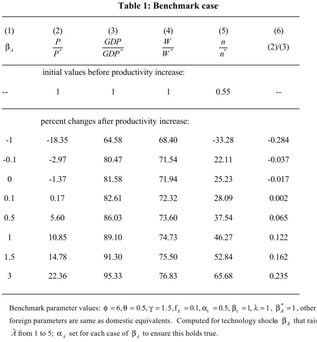
rises) in response to a ceteris paribus increase in the wage-adjusted effective productivity of its exports A W%_X / _{. The logic behind this result is similar to that behind the standard} Balassa-Samuelson result of real appreciation in response to a relative increase in the productivity of tradables. Conversely, consider a ceteris paribus increase in /A W% , holding A W%_X / _constant. Such a productivity change amounts to a productivity improvement biased towards nontradable goods and is associated with a real depreciation (fall in _{P P/} *₎

In general, the reduced form response of the real exchange to productivity changes depends on the relative wage change and the endogenous adjustment of tradability of goods. Further insight can be obtained by assuming Cobb-Douglas preferences over domestic and foreign goods (γ =1)18_{. The analogue expression for the real exchange rate is then}

[

]

(

)

(

)

1 * * 2 1 * * _{* * *} ; ; X A A X A n A P W P W A A n θ θ θ _{ω ω} ω ω − − _{  }     _{    } = _ _{        }         % % % (40)

where the notation reflects the dependence of productivity averages on the parameters of the productivity distribution as well as the share of nontraded goods. In the case that θ =1/2 and equal weights are placed on domestic and foreign goods, this simplifies further to

[

]

1/2 * * 1 / 2 * * * ; ; X X A A A n A n P P A A ω ω ω ω    _ _     =_{   }             % % % %

17 _{In the presence of proportional trade costs affecting all goods equally, 1,} * _1, * ₀

τ τ τ τ α < α < β =β = , then * * * , X T X T A% =αA% A% =α A%

In this case the real exchange rate is independent of relative wages since with Cobb-

Douglas preferences each country always spends the same amount on consumption. As in the more general case, the real exchange rate appreciates if export sector productivity rises relative to the economy average , i.e. A%X/A% rises.

Consider an increase in β_A which biases productivity increases towards export goods relative to the economy average, holding the foreign productivity parameters constant. This effect alone would tend to raise the real exchange rate in the condition above : while the rise in

productivity raises the average for all goods A% as well as the average for exported goods A%_X

alone, by construction it raises the latter more. Further, from the discussion in the previous section (see eqn. (34), we know an increase in βA that raises

*

ω ω> will tend to raise n relative to *

n .19 _{This means that the least productive of the traded goods are cut from that group, inducing} an even greater change in A%_X relative to A%, and thus an even larger increase in the real exchange rate. Hence endogenous changes in nontradability magnify the effect of productivity changes on the real exchange rate.

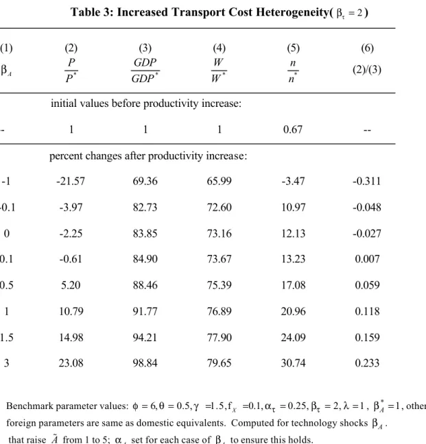
Consider next the case of a rise in transport cost heterogeneity; in particular, suppose a rise in β_τ which raises iceberg costs for all home goods, but in a biased way concentrated on those goods already with large costs (through an accompanying decline in α_τ). As in the case of a higher βA, the rise in βτ will raise

*

ω ω> and will tend to raise n relative to _n* _{(see (34)}

again), implying specialization in fewer traded varieties in Home rather than the foreign country. Since trade is being concentrated on more productive goods, this endogenous change in n also 18 _{Specifically, assume}

( )

( )

1 H FT P= P θ P −θ,

( ) ( ) (

1 _{/ (1 )}1

)

_{, 1 0} H FT C₌ C θ C −θ _θθ _−θ −θ _{> >θ .} 19

From (34) we see that the relation between _{ω ω,} * _{and n n,} * _{depends also on relative wages. To see that}

this does not affect the logic in the text, note that with Cobb-Douglas preferences over domestic and foreign goods and balanced trade, * *

PC=P C and

(

)

(

)

* * * (1 ) (1 ) F X H X L n f W W L n f − − =

− − (see (30) and (30*). Hence

with equal fixed export costs ( *

X X

f = f ) and labor supplies (L_H =L_F =L) across countries, (34) then reduces to _;

(

_{(1 )}

)

*_; *

(

₍₁ *₎

)

X X

X n_+ ω−_ L− −n f =X n_+ ω− _ L− −n f

    . We again see the property that

* _{n n}*_, * _{n n}*