No. 2004/13
Optimal Monetary Policy under
Commitment with a Zero Bound on
Nominal Interest Rates
Klaus Adam and Roberto M. Billi
Center for Financial Studies
The
Center for Financial Studies is a nonprofit research organization, supported by an
association of more than 120 banks, insurance companies, industrial corporations and
public institutions. Established in 1968 and closely affiliated with the University of
Frankfurt, it provides a strong link between the financial community and academia.
The CFS Working Paper Series presents the result of scientific research on selected
top-ics in the field of money, banking and finance. The authors were either participants in
the Center´s Research Fellow Program or members of one of the Center´s Research
Pro-jects.
If you would like to know more about the Center for Financial Studies, please let us
know of your interest.
1Klaus Adam, CEPR, London, University of Frankfurt, Mertonstr.17, PF94, 60054 Frankfurt am Main, Germany
2Roberto M. Billi, University of Frankfurt, Mertonstr.17, PF94, 60054 Frankfurt am Main, Germany
Thanks go to Kosuke Aoki, Joachim Keller, Albert Marcet, Ramon Marimon, Athanasios Orphanides, Volker Wieland, Mike Woodford, and participants at the CEPR-INSEAD conference on “Monetary Policy
CFS Working Paper No. 2004/13
Optimal Monetary Policy under Commitment with a Zero
Bound on Nominal Interest Rates
Klaus Adam
1and Roberto M. Billi
2First Version: March 24, 2003
This Version: April 1, 2004
Abstract:
We determine optimal monetary policy under commitment for a sticky price model with
monopolistic competition when nominal interest rates are bounded below by zero. The lower
bound causes the model to be nonlinear due to an occasionally binding constraint. A
calibration to the U.S. economy suggests that policy should reduce nominal interest rates
more aggressively than suggested by a model without lower bound: rational agents anticipate
the possibility of reaching the lower bound in the future and thereby amplify the effects of
adverse shocks. While the empirical magnitude of U.S. mark-up shocks seems too small to
entail zero nominal interest rates, real rate shocks plausibly lead to a binding lower bound
under optimal policy. This, however, occurs quite infrequently given the variability of U.S.
real rate shocks during past 2 decades. Interestingly, the presence of binding real rate shocks
requires to alter the policy response to (non-binding) mark-up shocks.
JEL Classification:
C63, E31, E52
Keywords:
nonlinear optimal policy, zero interest rate bound, commitment, liquidity trap,
New Keynesian
1
Introduction
This paper studies optimal monetary policy taking into account that nominal interest rates cannot be set to negative values.1 Considerable attention has recently been given to the policy implications of the lower bound on nominal interest rates, since these in major world economies are either already at or getting closer to zero.
A situation in which nominal interest rates are close to zero is gener-ally deemed problematic as the inability to further lower them can lead to higher than desired real interest rates. In particular, it is often feared that when agents hold deflationary expectations the economy might embark on a deflationary path, sometimes referred to as a ‘liquidity trap’, with high real interest rates generating demand shortfalls and thereby fulfilling the expectations of falling prices.
We consider optimal monetary policy under commitment in a micro-founded model with monopolistic competition and sticky prices in the prod-uct market (see Clarida, Galí and Gertler (1999) and Woodford (2003)). While the model we employ has been widely used to study optimal mone-tary policy and short-run fluctuations, we seem to be the first to analyze it on a fully stochastic setup that takes into account the zero lower bound. This is of interest because, as we show, the presence of shocks generates qualitatively new features of optimal monetary policy that do not appear when either ignoring the lower bound or assuming perfect foresight. In ad-dition, a stochastic model can be calibrated to real world economies. This allows us to assess the quantitative implications of the zero lower bound for U.S. monetary policy.
We should mention that solving the stochastic rational expectations equi-librium of our model is not trivial as it involves occasionally binding con-straints.2 Our numerical technique is based on the insights of Marcet and Marimon (1998) and requires solving for the functionalfixedpoint of a gen-eralized Bellman equation. To our knowledge we are the first to solve for the saddle point function that solves this Bellman equation. While our so-lution method is complementary to the approach of Christiano and Fisher
1In principle negative nominal rates are feasible, e.g., if one is willing to give up free convertability of deposits and otherfinancial assets into cash or if one could levy a tax on money holdings, see Buiter and Panigirtzoglou (2003), Goodfriend (2000). However, these policy measures are generally considered to be practically inapplicable.
(2000) that is based onfirst order conditions, it has the paramount advan-tage that we can check whether second order conditions hold. In particular, we numerically verify the saddle point property of our solution which is a sufficient condition for having found a constrained maximum.
Two qualitatively new features of optimal policy emerge from this anal-ysis.
First, we find that nominal interest rates are lowered more aggressively in response to a fall in the natural real interest rate than what is suggested instead by a model without lower bound.3 Such ‘preemptive’ easing of nom-inal rates is optimal because agents anticipate the possibility of binding real rate shocks in the future and reduce their output and inflation expectations correspondingly. Such expectations end up amplifying the adverse effects of real rate shocks and thereby trigger a stronger policy response. Since this will cause the bound to be hit earlier, there exists a complementarity between private sector expectations and the optimal policy reaction to such expectations.4
Second, the presence of real rate shocks that cause the zero lower bound to bind also alters the optimal policy reaction to (non-binding) mark-up shocks. This occurs because the policymaker cannot affect the average real interest rate in any stationary equilibrium, therefore, faces a ‘global’ policy constraint. The inability to lower nominal and real interest rates as much as desired then requires that optimal policy increases rates less (or lowers rates more) in response to non-binding shocks compared to the policy that would be optimal in the absence of the lower bound.
There are also a number of quantitative results regarding optimal U.S. monetary policy and the relevance of the zero lower bound emerging from this analysis.
First, the zero lower bound appears inessential in dealing with mark-up shocks, i.e., variations over time in the degree of monopolistic competition betweenfirms.5 More precisely, the empirical magnitude of mark-up shocks in the U.S. economy observable for the period 1983-2002 is too small for
3The natural real rate is the real interest rate associated with the optimal use of productive resources underflexible prices.
4Although we do not formally show the existence of sunspot equilibria, this comple-mentarity may be troublesome for policy making in practice.
the zero-lower bound to become binding. This would remain the case even when the true variance of mark-up shocks were threefold above our estimated value.
Second, the shocks to the ‘natural’ real rate of interest may cause the lower bound to become binding, but this happens relatively infrequently and is a feature of optimal policy. Based on our estimates for the 1983-2002 period, in the U.S. economy the bound would be expected to bind on average in about one quarter every 17 years under optimal policy.6 Moreover, once zero nominal interest rates are observed they are expected to endure on average not more than 1 to 2 quarters. Also, the average welfare losses entailed by the zero lower bound seem rather small for the U.S. economy.
The latter results, however, are sensitive to the size of the standard deviation of the estimated real rate process. In particular, we find that zero nominal rates would occur much more frequently and generate higher welfare losses if the real rate process had a somewhat larger variance.
Third, as argued by Jung, Teranishi, and Watanbe (2001) and Eggertsson and Woodford (2003) optimal policy reacts to a binding zero lower bound on nominal interest rates by creating inflationary expectations in the form of a commitment to let future output gaps and inflation rates increase above zero. The policymaker thereby effectively lowers the real interest rates that agents are confronted with. Since reducing real rates using inflation is costly (in welfare terms), the policymaker has to trade-offthe losses generated by too high real rates with those stemming from higher inflation rates.
We find that the required levels of inflation and the associated positive output gap are very moderate. A negative 3 standard deviation shock to the natural real rate requires a promise of an increase in the annual inflation rate in the order of 15 basis points and a positive output gap of roughly 0.5%.
Finally, while the optimal policy response to shocks through the promise of above average output and inflation may in principal generate a ‘commit-ment bias’, the quantitative effects turn out to be negligible. This holds not only for our baseline calibration but also for a range of alternative model
6
parameterizations. It suggests that optimal policy for the U.S. economy im-plements an average inflation rate of zero even when taking direct account of the zero lower bound on nominal interest rates.7
The remainder of this paper is structured as follows. Section 2 briefly discusses the related literature. Thereafter, section 3 introduces the model and the policy problem. In section 4 we prove the model’s ability to generate a ‘liquidity trap’, i.e., deflation and negative output gaps in the presence of zero nominal interest rates. Section 5 presents our calibration for the U.S. economy and explains how the historical shock processes were identified. The solution method we employ is described in section 6. Section 7 presents our main results on optimal monetary policy with lower bound for the U.S. economy. We then discuss in section 8 the robustness of our findings to various parameter changes, and briefly conclude in section 9.
2
Related Literature
A number of recent papers study the implications for optimal monetary policy of the zero lower bound on nominal interest rates.
Most closely related is Eggertsson and Woodford (2003) who consider a perfect foresight economy and analytically derive optimal targeting rules with a lower bound. In this paper we consider a fully stochastic setup and solve the model numerically. A stochastic setup has two important advantages. First, it allows for the possibility that shocks drive the economy from a non-binding region into a region where the lower bound is binding. This allows to assess how policy should be conducted in the ’run-up’ to a binding situation. Secondly, a stochastic setup allows us to calibrate the model to actual economies and to study the quantitative importance of the zero lower bound for the conduct of monetary policy in practice.
A related set of papers focuses on optimal monetary policy in the ab-sence of credibility. In a companion paper Adam and Billi (2003) derive the nonlinear optimal policy under discretion for a stochastic New Keynesian model calibrated to the U.S. economy. Instead, Eggertsson (2003) analyzes discretionary policy and the role of nominal debt policy as an instrument to achieve credibility.
7Zero inflation is optimal because it minimizes the price dispersion betweenfirms with sticky prices and we abstract from the money demand distortions associated with positive nominal interest rates.
The performance of simple monetary policy rules is examined by Fuhrer and Madigan (1997), Orphanides and Wieland (1998), and Wolman (2003). A main finding of these papers is that if the targeted inflation rate is close enough to zero policy rules formulated in terms of inflation rates, e.g., the Taylor rule (1993), can generate significant real distortions. Reifschneider and Williams (2000) and Wolman (2003) show that simple policy rules for-mulated in terms of a price level target can significantly reduce these real distortions associated with the zero lower bound on interest rates. Benhabib et al. (2002) study the global properties of Taylor-type rules showing that these might lead to self-fulfilling deflations that converge to a low inflation or deflationary steady state. Evans and Honkapohja (2003) study the prop-erties of global Taylor rules under adaptive learning, showing the existence of an additional steady state with even lower inflation rates.
The role of the exchange rate and monetary-base rules in overcoming the adverse affects of a binding lower bound on interest rates is analyzed, e.g., by Auerbach and Obstfeld (2003), Coenen and Wieland (2003), McCallum (2003), and Svensson (2003).8
3
The Model
We consider a simple and well known monetary policy model based on a representative consumer and firms in monopolistic competition facing re-strictions on the frequency of price adjustments (Calvo (1983)). Following Rotemberg (1987) this is often referred to as the ‘New Keynesian’ model and has frequently been studied in the literature, e.g., Clarida, Galí and Gertler (1999) and Woodford (2003).
3.1
Private Sector
The behavior of the private sector is described by two linearized equations.9 On the one hand, profit maximizing price setting behavior byfirms implies an ‘aggregate supply’ (AS) equation of the form
πt=βEtπt+1+λyt+ut (1)
8Further articles dealing with the relevance of the zero lower bound can be found in the special issues of the Journal of Japanese and International Economies Vol. 14, 2000 and the Journal of Money Credit and Banking Vol. 32 (4,2), 2000.
9We justify the use of linearized equations in section 3.3.3 based on the computational complexity of numerically solving the model.
where πt denotes the inflation rate from period t−1 to t and yt is the
deviation of output from its natural rate.10 The shock ut captures the
stochastic variation in the degree of substitutability between different goods that leads to variation in the mark-up charged by firms.11 The parameter β ∈ (0,1) is the discount factor and λ > 0 indicates how strong is the reaction of inflation to deviations of output from its natural rate.
On the other hand, the Euler equation describing households’ optimal labor and consumption decisions delivers an ‘IS curve’ of the form
yt=Etyt+1−ϕ(it−Etπt+1) +gt (2)
where it denotes the nominal interest rate (in deviation from the interest
rate consistent with the zero inflation steady state) andϕ>0is the interest rate elasticity of output. The shockgtcaptures the variation in the ‘natural’
real interest rate, i.e.,
gt=ϕ(rt−r∗) (3)
where rt is the real rate consistent with the flexible price equilibrium and
r∗= 1/β−1is the real rate of the deterministic zero inflation steady state. The shock gt summarizes all shocks that generate time variation in the
real interest rate under flexible prices, therefore, captures the combined effects of preference shocks, productivity shocks, and changes in government expenditure.12
The laws of motion of the shocks are assumed to be given by
ut=ρuut−1+εu,t (4)
gt=ρggt−1+εg,t (5)
with ρj ∈ (−1,1) and εj,t ∼ iiN(0,σj2) for j = u, g. As will be shown in
the following sections, this specification of the shock processes is sufficiently general to describe the historical sequence of shocks in the U.S. economy for the period 1983:1-2002:4 that we consider.
1 0
The natural rate of output is the output level that would emerge if prices wereflexible. 1 1See Steinsson (2003) for details.
3.2
Monetary Authority
We suppose that the monetary authority controls the short-term nominal interest rate it, but control is subject to a lower bound that emerges from
the presence of money that offers a zero nominal return. This implies that nominal interest rates are non-negative, which in terms of our notation is captured by the restriction
it≥ −r∗. (6)
We further assume that the monetary authority uses nominal interest rates to maximize the welfare of the representative agent. As shown in Woodford (2001), this can be approximated by a quadratic function in output and inflation Wt=−Et "∞ X i=0 βi¡πt2+i+αyt2+i¢ # (7)
where the weightα>0depends on the underlying preference and technology parameters.
Intuitively, the welfare function captures the following two effects. Firstly, output gaps are inefficient because they denote deviations of output from the (approximately efficient) natural rate of output. Secondly, inflation is inefficient because it generates price dispersion between firms that cannot perfectly adjust prices, thereby induces socially inefficient substitution be-tween the goods produced by different entrepreneurs.13
Therefore, the monetary policy problem is the following
1 3Substitution is socially inefficient becausefirms face increasing marginal costs of pro-duction and labor is imperfectly substitutable between different varieties.
max {yt,πt,it} −E0 "∞ X t=0 βt¡π2t +αyt2¢ # (8) s.t.: πt=βEtπt+1+λyt+ut (9) yt=Etyt+1−ϕ(it−Etπt+1) +gt (10) it≥ −r∗ (11) ut=ρuut−1+εu,t (12) gt=ρggt−1+εg,t (13) u0,g0 given
Note that besides setting interest rates, the monetary authority is allowed to ‘choose’ the associated output gaps and inflation rates. This implies that whenever there exist multiple rational expectations equilibria consis-tent with a given interest rate policy the economy coordinates on the welfare superior equilibrium. As shown in Woodford and Giannoni (2003) such co-ordination may be achieved by conditioning policy on endogenous variables in an appropriate way.
3.3
Discussion
3.3.1 Money demand distortions
The objective function (7) does not contain any element capturing the dis-tortionary effects of positive nominal interest rates, an issue that has been emphasized by Milton Friedman. It thus implicitly assumes that real money balances are of negligible importance (in utility terms) and the distortion generated by positive nominal interest rates can be abstracted from. One may interpret this in the sense of a cash-less limit economy, as in Woodford (1998).
We note that the neglect of money balances, in any case, does not seem to entail a significant approximation error. Schmitt-Grohé and Uribe (2003a), e.g., find that price level stability should indeed be the overriding policy objective in the presence of sticky prices, even when taking into account the distortions generated by positive nominal interest rates.
3.3.2 Policy instruments
By assuming that the interest rate is the only available policy instrument we deliberately abstract from a number of alternative policy channels, most notably fiscal policy, exchange rate policy, and quantity-based monetary policies.
While the omission of fiscal policies clearly constitutes a shortcoming that ought to be addressed in future work, ignoring exchange rate and money policies may be less severe than one might initially think. Clarida, Galí and Gertler (2001), for example, show that one can reinterpret the present model as an open economy model and there exists a one-to-one mapping be-tween interest rate policies and exchange rate policies. It is then inessential whether policy is formulated in terms of interest rates or exchange rates. Similarly, ignoring quantity-oriented monetary policies in the form of open market operations during periods of zero nominal interest rates seems to be of little relevance. Eggertsson and Woodford (2003) show that in the present model such policies have no effect on the equilibrium unless they influence the future path of interest rates.
We recognize that alternative policy instruments may still be relevant in practice.14 Focusing on interest rate policy in isolation is nevertheless of considerable interest as it allows to assess what interest rate policy alone can achieve in avoiding liquidity traps and whether there is any need for employ-ing alternative instruments. This seems important to know, given that these alternative instruments are often subject to (potentially uncertain) political approval by external authorities and may therefore not be readily available.
3.3.3 How much non-linearity?
Instead of the fully nonlinear model, we use linear approximations to thefirst order conditions, i.e., equations (1) and (2), and a quadratic approximation to the objective function, i.e., equation (7). Doing so means that the only nonlinearity that we take account of is the one imposed by the zero lower bound (6). Technically, this approach is equivalent to linearizing the first order conditions of the nonlinear Ramsey problem around the first best steady state except for the non-negativity constraint for nominal interest rates that is kept in its original nonlinear form. This approximation is valid for small shocks and whenver the steady state interest rate is sufficiently
1 4
See Eggertsson (2003) on how other policy instruments, e.g., nominal debt policy, may be used as a commitment device.
close to the zero lower bound, i.e., when the quarterly discount factor β is sufficiently close to one.
Clearly, this modelling approach has advantages and disadvantages. One disadvantage is that for the empirical shock support and the actual value of the discount factor the linearizations (1) and (2) may perform poorly. However, this depends on the degree of nonlinearity present in the economy, an issue about which relatively little seems to be known empirically.
A paramount advantage of our approach is that one can economize in the dimension of the state space. A fully nonlinear setup would require instead an additional state to keep track over time of the higher-order effects of price dispersion, as shown by Schmitt-Grohé and Uribe (2003b). Computation costs would become prohibitive with an additional state.15
A further advantage of focusing on the nonlinearities induced by the lower bound only is that one does not have to parameterize higher order terms when applying the model to the U.S. economy. This seem important, given the lack of evidence about the empirical importance of such terms.
Finally, the simpler setup implies that our results remain more easily comparable to the standard linear-quadratic analysis without lower bound as the only difference consists of imposing equation (6).
4
Zero Bound and Liquidity Traps
In this section we assess the suitability of the simple model described in the previous section for studying issues related to the zero lower bound and ‘liquidity traps’.
We believe that a minimum requirement of any model used to analyze these issues is that it should be able to replicate the Japanese experience of the 1990s, i.e., low nominal interest rates, deflation, and negative output gaps. It is precisely the apparent existence of such unfavorable ‘liquidity trap equilibria’ that causes the zero lower bound to be of economic interest.
For this reason we determine the set of Rational Expectations Equilibria (REE) consistent with equations (1) and (2) whenit≡ −r∗, i.e., when
nom-1 5
For our version of the model we have 4 state variables with continuous support. We need a considerable amount of (collocation) nodes along most of the dimensions to appro-priately capture the kinds in the policy functions. The models with occasionally binding constraints analyzed by Christiano and Fisher (2000) had one or two state variables at most.
inal interest rates are at their lower bound.16’17 We then analyze whether there exist REE that display properties associated with a liquidity trap, as defined above. In the appendix the following result is derived:
Proposition 1 (REE with Zero Bound) Suppose it = −r∗ for all t. The
full set of Rational Expectations Equilibria for the model described by equa-tions (1) and (2) is given by
• a continuum of locally explosive solutions, possibly involving sunspots, where either output is positive and inflation negative or output negative and inflation positive.
• a set of stationary solutions
µ πt yt ¶ = µ −r∗ −1−λβr∗ ¶ +Γ µ ut gt ¶ + ∞ X n=0 φn µ ω 1 ¶ st−n (14) where Γ= Ã −1+ρu ρuϕλ+ρu−1+ρuβ−ρ2uβ −λ −1+ρg+ρgϕλ+ρgβ−ρ2gβ −ρuϕ ρuϕλ+ρu−1+ρuβ−ρ2uβ −1+ρgβ −1+ρg+ρgϕλ+ρgβ−ρ2gβ ! (15)
and the sunspot variable st∈R1 is an arbitrary martingale difference
series, φ∈(0,1), and ω>0.
Clearly, the locally explosive solutions mentioned in proposition 1 seem inadequate explanations of liquidity traps, as either inflation or output are increasing.18 Moreover, such equilibria are Pareto dominated by the sta-tionary equilibria since the rate of growth of output or inflation is (locally) larger than1/β, see the appendix.
The situation is different for the stationary solutions (14).19 Since the coefficients in the respective columns ofΓ have the same sign, when interest
1 6
Whenβis sufficiently close to one the linearization of equations (1) and (2) remains valid atit=−r∗,sincer∗= 1β−1→0asβ→1.
1 7We assume transversality conditions to be satisfied. Subsequent footnotes discuss various aspects of this assumption.
1 8Since we use a linearized model, these variables need not increase without bound in the underlying fully nonlinear model, i.e. one cannot rule out such equilibria based on feasibility arguments. Yet, provided the solutions exist in the nonlinear model, they will display either high inflation or high output and are therefore unable to replicate a liquidity trap.
1 9As argued in Eggertsson and Woodford (2003) such solutions statisfy the transversality constraint iffiscal policy contracts the stock of outstanding goverment debt at a sufficient rate. This is the case, for example, iffiscal policy is Ricardian.
rates are at their lower bound mark-up shocks and demand shocks can give rise to both low output and low inflation. Clearly, similar phenomena may be generated by sunspot shocks, since ω > 0. Solutions of the form (14), thus, have the potential to replicate the Japanese experience of the recent years.
In the remaining part of the paper we will focus on stationary funda-mental equilibria. These equilibria Pareto dominate explosive equilibria and any equilibria involving sunspots, and may generate equilibrium paths re-sembling liquidity traps. Moreover, since the stationary fundamental solu-tion is locally isolated among the set of fundamental rasolu-tional expectasolu-tions solutions, learning dynamics may be expected to select the stationary so-lution instead of the explosive soso-lutions, as in the analysis of Evans and Honkapohja (2003) with a related model.
As afinal remark, we should point out that the model is globally stable, in the sense that there always exist feasible interest rate policies consis-tent with a stationary equilibrium path. This differs from earlier studies, e.g., Orphanides and Wieland (2000), in which for some realizations of the shocks the economy possesses only destabilizing equilibria. The global sta-bility property of the present set up, however, might be sensitive to the introduction of lagged inflation terms in the price setting equation (1), a question that would have to be explored in future work.
5
Model Calibration
To asses the quantitative importance of the zero lower bound for monetary policy in the U.S. economy we need to assign values to the model parameters. In particular we must choose parameter values for the coefficients appearing in equations (8), (9), (10), (12) and (13).
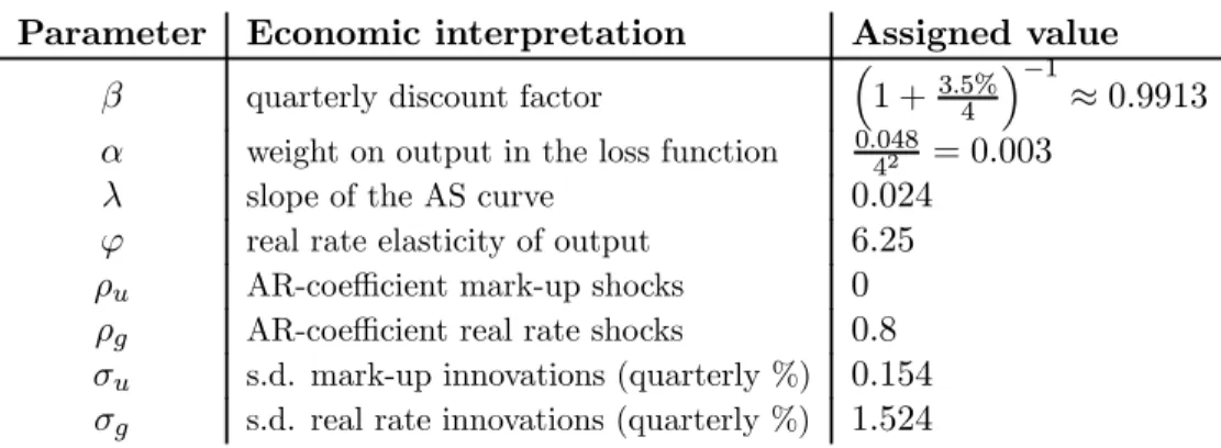
Table 1 summarizes our parameterization for the U.S. economy. The values for α, λ, and ϕ are taken from table 6.1 in Woodford (2003), based in turn on Rotemberg and Woodford (1998). Instead, the parameters of the shock processes and the discount factor are estimated using U.S. data for the period 1983:1-2002:4.
Parameter Economic interpretation Assigned value
β quarterly discount factor
³
1 +3.5%4 ´−1 ≈0.9913
α weight on output in the loss function 0.40482 = 0.003
λ slope of the AS curve 0.024
ϕ real rate elasticity of output 6.25
ρu AR-coefficient mark-up shocks 0
ρg AR-coefficient real rate shocks 0.8
σu s.d. mark-up innovations (quarterly %) 0.154
σg s.d. real rate innovations (quarterly %) 1.524
Table 1: Parameter values (baseline calibration)
The estimation procedure follows Rotemberg and Woodford (1998). We
first construct output and inflation expectations by estimating expectation functions from the data. Then we plug these expectations along with actual values of the output gap and inflation into equations (1) and (2) and identify the shocksut andgt with the equation residuals.
We measure output by linearly detrended log real GDP, and inflation by the log quarterly difference of the implicit deflator.20 Detrended output
is depicted in figure 1. For the interest rate we use the quarterly average of the fed funds rate in deviation from the average real rate for the whole sample, which is approximately equal to3.5%(in annual terms). Based on this latter estimate we set the quarterly discount factor shown in table 1.21
All variables used are expressed in percentage terms. When presenting results we transform quarterly inflation rates and interest rates into annual rates.22
The expectations in equations (1) and (2) are constructed from the pre-dictions of an unconstrained VAR in output, inflation, and the fed funds
2 0
The data is taken from the Bureau of Economic Analysis: www.bea.gov. Using quadratically detrended GDP or HP(1600)-filtered GDP leaves the estimated parameters of the shock processes virtually unchanged.
2 1
We implicitely assume that the positive inflation rates displayed in the sample did not affect the real rate so that the nominal interest rate in the zero inflation steady state remains equal to this real rate.
rate with three lags.23 The correlations of the VAR residuals are depicted in
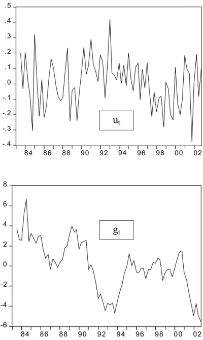
figure 2. Substituting these VAR predictions for the expectations in equa-tions (1) and (2) one can then identify the shocks ut and gt. The implied
shock series are shown infigure 3.
While the mark-up shocks ut seem to be close to white noise, the real
rate shocksgtare rather persistent. As one would expect, the real rate seems
to fall during recessions, e.g., at the beginning of the 1990’s and at the start of the new millennium. Fitting univariate AR(1) processes to these shocks delivers the following estimates24
ρu= 0.129 (0.113)
ρg = 0.919 (0.050)
σu= 0.153
σg = 1.091
The estimated value of ρu is insignificant at conventional significance
lev-els.25 For this reason we use ρu = 0 and set the standard deviation of
the innovations εu,t so as to match the standard deviation of the identified
mark-up shocks, which is approximately equal to0.61%annually.
The estimate ofρg indicates that real rate shocks are highly persistent.26
The implied annual standard deviation of the real rate, as implicitly defined in equation (3), is equal to 1.63%.27 Although real rate shocks seem quite
2 3Estimating expectations functions in such a way is justified as long as there are no structural breaks in the economy. Since our sample period, 1983:1-2002:4, starts after the disinflation policy under Federal Reserve chairman Paul Volcker, monetary policy is expected to have been reasonably stable, see Clarida et al. (2000). A VAR lag order selection test based on the Akaike information criterion with a maximum of 6 lags suggests the inclusion of 3 lags. A Wald lag exclusion test indicates that the third lags are jointly significant at the 2% level.
2 4Numbers in brackets are the standard errors of the point estimates. The univariate AR(1) describe the shock processesut andgt quite well. In particular, there is no
signif-icant autocorrelation left in the innovationsεi,t (i=u, g). Also when estimating AR(2)
processes the additional lags remain insignificant.
2 5This contrast with Ireland (2002) who uses data starting in 1948:1. Extending our sample back to this date would also lead to highly persistent mark-up shocks. Since we do not argue that monetary policy has been constant across the extended sample, we choose the shorter period commencing in 1983:1.
2 6
This is similar to the results in Ireland (2002).
2 7When using instead the period 1979:4-1995:2 as in Rotemberg and Woodford (1998), which includes the volatile years 1980-1982, wefind for the estimated real rate process an annual standard deviation of 2.57%.
persistent, the persistence drops considerably once one uses future actual values to identify output and inflation expectations in equations (1) and (2).28 The estimated autoregressive coefficient for the real rate shocks then drops to ρg = 0.794 which indicates that forecasts that are better than
our simple VAR-predictions would most likely lead to a reduction in the estimated persistence.29 For this reason we setρg = 0.8in our calibration.30
Finally, the standard deviation of the innovationsεg,tin table 1 is chosen
again so as to keep the unconditional standard deviation of the calibrated real shock process equal to the standard deviation of the identified shock values.
6
Solving the Model
Due to the presence of the zero lower bound analytical results for optimal interest rate policy are unavailable. For this reason we have to rely on numerical methods.
An important complication that arises, however, is that the policy-maker’s maximization problem (8) fails to be recursive, since constraints (9) and (10) involve forward-looking variables. For this reason dynamic programming techniques cannot be applied directly; these assume transi-tion equatransi-tions that do not involve expectatransi-tion terms. To obtain a dynamic programming formulation of problem (8) we apply the technique of Marcet and Marimon (1998) and reformulate the problem as follows:
W(µ1t, µ2t, ut, gt) = inf γ1 t,γt2 sup yt,πt,it © h(yt,πt, it,γt1,γt2, µ1t, µ2t, ut, gt) +βEt £ W(µ1t+1, µt2+1, ut+1, gt+1) ¤ª (16) 2 8
This amounts to assuming perfect foresight. 2 9
When using VAR-predictions but considering the period 1979:4-1995:2, as in Rotem-berg and Woodford (1998), the point estimate also drops toρg = 0.827.
3 0
This value cannot be rejected at the 1% significance level when using estimates based on the VAR-expectations. In an earlier version of the paper, which is available upon request, we used instead the point estimates forρuandρg.
s.t.: it≥ −r∗ µ1t+1=γt1 µ2t+1=γt2 ut+1 =ρuut+εu,t+1 gt+1=ρggt+εg,t+1 µ10 = 0 µ20 = 0 u0, g0 given where h¡y,π, i,γ1,γ2, µ1, µ2, u, g¢ ≡ −αy2−π2+γ1(π−λy−u)−µ1π +γ2(y+ϕi−g)−µ2 1β(ϕπ+y). (17) Problem (16) is fully recursive as all transition equations now involve only lagged state variables.
A crucial feature of the reformulated problem (16) is that it introduces two co-state variables(µ1, µ2)bringing the total number of state variables up to four. The states(µ1, µ2)are the lagged values of the Lagrange multipliers for the constraints (9) and (10), respectively; they can be interpreted as ‘promises’ that have to be kept from past commitments. A negative value ofµ1, e.g., indicates a promise to generate higher inflation rates than what purely forward looking policy would imply.31 Likewise, a negative value of
µ2indicates a promise to generate higher values of β1(ϕπ+y)than suggested by purely forward looking policy.
We then apply numerical dynamic programming tools to approximate the value function that solves the recursive saddle point functional equation (16) and derive the associated policy functions.32 It appears that we are
the first to actually solve for the saddle point function of such a recursive
3 1
This follows from the expression of the one-period return functionh(·)given in equa-tion (17).
3 2
In particular, we use the collocation method with cubic splines as basis functions to approximate the value function solving equation (16). For details on projections methods and the collocation method see Judd (1998). We iterate on the Bellman equation until the maximum absolute change in the basis coefficients falls below the square root of machine precision, i.e., approximately 1.49·10−8. The accuracy of our numerical solution is then checked by studying the Bellman equation residuals on afine grid offthe collocation nodes. With this procedure and some experimentation, we choose the collocation nodes so as to minimize on the Bellman equation residuals. Solutions have been computed in MatLab employing the toolboxes of Miranda and Fackler (2002).
problem. Our solution method is complementary to the ones studied by Christiano and Fisher (2000) who focused on first order conditions but has the paramount advantage that it allows to verify second order conditions. In particular, we numerically check whether the right-hand side of (16) has a saddlepoint in the variables(γt1,γt2) and(yt,πt, it), respectively, at the
con-jectured optimal solution. As is well known, e.g. chapter 14.3 in Silberberg (1990), the saddle point property is a sufficient condition for having found a constrained optimum. The results of this solution approach are reported in the next sections.
7
Optimal Policy with Lower Bound
This section shows the optimal policy with a lower bound on nominal interest rates for the model calibrated to the U.S. economy.
Before presenting the results we would like to emphasize that the pres-ence of the zero lower bound generates nonlinear optimal policies therefore causes a failure of certainty-equivalence. This has two important implica-tions. First, the average value of endogenous variables will generally differ from the steady state value in a way that depends on the nature of the shocks. Second, the average or expected model dynamics in response to shocks will differ from the deterministic impulse responses. For this latter reason we discuss results in terms of the implied ‘mean dynamics’ in response to shocks, instead of the more familiar deterministic impulse responses.33
7.1
Optimal Policy Functions
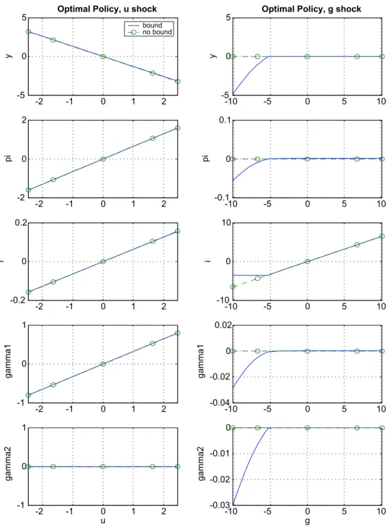
Figure 4 presents the optimal responses of(y,π, i) and the Lagrange multi-pliers(γ1,γ2)to a mark-up shock and a real rate shock.34 The responses of
the Lagrange multipliers are of interest because they represent commitments regarding future inflation rates and output levels, as explained in the pre-vious section. Depicted are the optimal policy responses both for the case of the zero lower bound being imposed (solid line) and for the case when interest rates are allowed to become negative (dashed line with circles).
3 3
Mean dynamics are identical to impulse responses whenever certainty equivalence holds, e.g., in the absence of the zero lower bound. We found that in our nonlinear model the mean dynamics differ considerably from the deterministic impulse responses.
3 4
The state variables not shown on thex-axes are set to their (unconditional) average values. Policies are shown for a range of ±4 unconditional standard deviations of both the mark-up shock and real rate shock.
The left-hand panel offigure 4 shows that the optimal response to mark-up shocks is virtually unaffected by the presence of the zero lower bound.35 Independently of whether the bound is imposed or not, a positive mark-up shock lowers output and leads to a promise of future deflation, as indicated by the positive value of γ1. The latter ameliorates the inflationary effect of the shocks through the expectational channel present in equation (1). To deliver on its promise the policymaker increases nominal interest rates.36
Yet, since the required interest rate changes are rather small, mark-up shocks do not plausibly lead to a binding lower bound.
The situation is quite different when considering the policy response to a real rate shock, which is shown on the right-hand panel offigure 4. With-out zero lower bound these shocks do not generate any policy trade-off: the required real rate can be implemented through appropriate variations in the nominal rate alone. Yet, once the lower bound is imposed sufficiently negative real rate shocks cause the bound to be binding. Promising future inflation is then the only remaining instrument for implementing reductions in the real rate. The negative values for γ1 and γ2 reveal that the policy
maker indeed commits to future inflation as a substitute for nominal rate cuts once the lower bound is reached. Yet, since inflation is a costly in-strument (in welfare terms), it would be suboptimal to completely undo the output losses generated by negative real rate shocks. As a result, there is a negative output gap, some deflation, and nominal interest rates are at their lower bound. Note that all these features are generally associated with a ‘liquidity trap’.
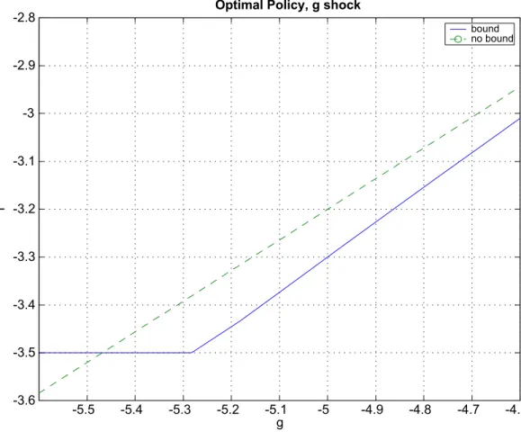
Figure 5 depicts the optimal interest rate response to real rate shocks in greater detail. This shows that once the lower bound is taken into account it is optimal to reduce nominal rates more aggressively than is the case when nominal rates are allowed to become negative. As a result of this ‘preemptive’ easing of nominal rates the lower bound is reached earlier than suggested by optimal policy without taking into account the lower bound.37
3 5The optimal reaction to mark-up shocks is different with or without the bound, but the difference is quantiatively small for the calibrated parameter values. We will come back to this point in section 7.4.
3 6
The sign of the optimal interest rate response, however, depends on the degree of autocorrelation of the mark-up shocks. In particular, with more persistent shocks nominal rates would optimally decrease in response to a positive mark-up shock.
3 7Kato and Nishiyama (2003) found a similar effect when using a backward looking AS curve which suggests that our result is robust to the introduction of lagged inflation terms into the ‘New Keynesian’ AS curve. Using different models, Orphanides and Wieland
A stronger interest rate reduction is optimal because the possibility of a binding lower bound in the future puts downward pressure on expected future output and inflation, since these variables become negative once the bound is reached, see the right-hand panel offigure 4. The reduced output and inflation expectations amplify the effects of negative real rate shocks in the IS equation (2) and thereby require that the policy maker lowers nominal rates faster than is the case without lower bound.
This anticipation effect points towards an interesting complementarity between policy decisions and private sector expectations that may be of considerable importance for actual policy making. Suppose, e.g., that agents suddenly assign a larger probability to the lower bound being binding in the future. This would lower output and inflation expectations, and in turn induces policy to reduce the nominal interest rate thereby causing the economy to move into the direction of the expected change. This points towards the existence of possible sunspot fluctuations, an issue that may have to be explored in future work.
7.2
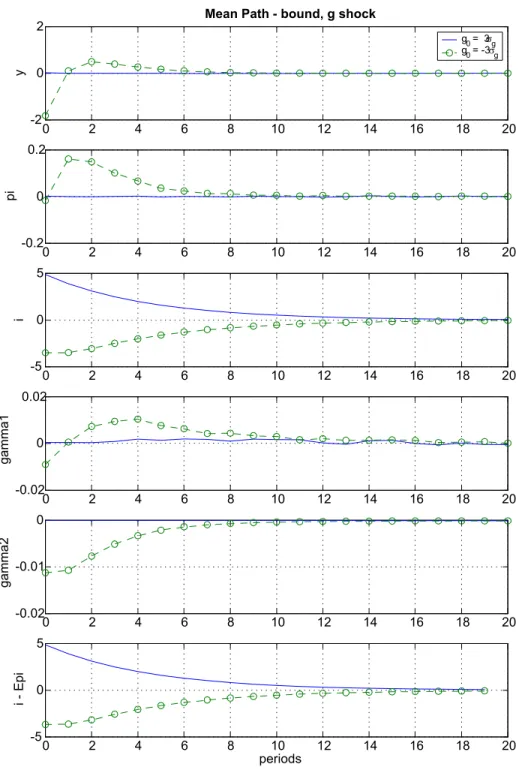
Dynamic Response to Real Rate Shocks
Figure 6 displays the mean dynamics of the economy in response to real rate shocks of±3unconditional standard deviations.38 With our calibration the annual ‘natural’ real rate, i.e., the real interest rate consistent with the efficient use of productive resources, then stands temporarily at+8.39%and
−1.39%, respectively; the interesting case being the one where full use of productive resources requires a negative real rate.
As argued by Krugman (1998), negative real rates are plausible even if the marginal product of physical capital remains positive. For instance agents may require a large equity premium, as historically observed in the U.S., or the price of physical capital may be expected to decrease.
Figure 6 shows that in response to a negative real rate shock annual inflation rises by about 15 basis points for 3 to 4 quarters and then returns to a value close to zero. Similarly, output increases slightly above potential
(2000) and Reifschneider and Williams (2000) also report more aggressive easing than in the absence of the zero bound.
3 8The initial values for the other states are set equal to their unconditional average values. Setting them to theconditional average values consistent with the real rate shock does not make a difference. The mean dynamics in this and other graphs are the average responses for 100 thousand stochastic simulations.
after the second quarter and slowly returns to potential. Getting out of a ‘liquidity trap’ induced by negative real-rate shocks, thus, requires that the policymaker promises to let future output and inflation increase above zero for a substantial amount of time. The qualitative feature of thisfinding has already been reported in Eggertsson and Woodford (2003), and in a some-what different form in Auerbach and Obstfeld (2003). Our results clarify, however, that the required amount of inflation and the output boom are rather modest.
Note, that ex-post there would be strong incentives to increase nominal interest rates earlier than promised as this would bring both inflation and output closer to their target values. The feasibility of the optimal policy re-sponse, therefore, crucially depends on the policymaker’s credibility. Wether policymakers can and want to credibly commit to such policies is currently subject of debate, see for example Orphanides (2003).
7.3
Frequency of Binding Rates and Welfare Implications
In this section we discuss the frequency with which the zero lower bound can be expected to bind and welfare implications. It turns out that for the calibration to the U.S. economy the lower bound binds rather infrequently, namely in about one quarter every 17 years on average. Moreover, zero nom-inal interest rates tend to prevail for rather short periods of time (roughly 1.4 quarters on average).
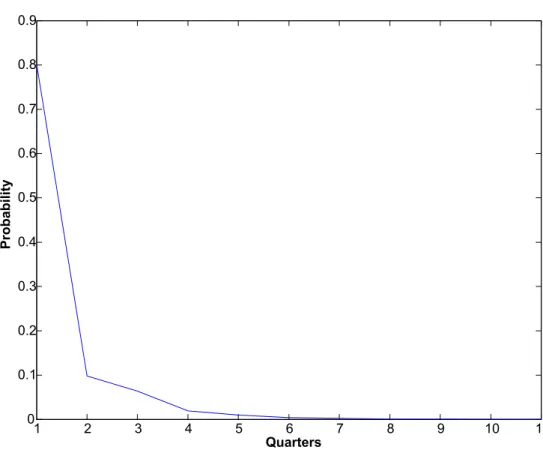
Figure 7 displays the probability with which under optimal policy the zero bound is binding for n quarters, conditional on it being binding in quarter one. The likelihood that zero nominal interest rates persist for more than 4 quarters is 1.8% only. Given that the lower bound is hit rather in-frequently, possible inflation and output biases emerging from the nonlinear policy functions are expected to be small. In fact, our simulations show that for the calibration at hand there are virtually no average level effects for output and inflation. Although output and inflation are somewhat larger than zero on average, for both variables the effects are in the order of less than 0.01%.
Finally, as one would expect, the average welfare effects generated by the existence of a zero lower bound are rather small. Our simulations show that the additional welfare losses of the zero lower bound are roughly 1%
of those generated by the stickiness of prices alone.39 Given that the zero lower bound is reached rather infrequently, however, this indicates that the conditional welfare losses associated with being at the lower bound are quite substantial.
7.4
Global Implications of Binding Shocks
This section reports a qualitatively newfinding that stems from the presence of binding negative real rate shocks. It turns out that the presence of binding shocks alters the optimal policy response to non-binding shocks, i.e., the reaction to positive real rate shocks and mark-up shocks of both signs. In this sense the existence of a lower bound has global implications on the shape of the optimal policy functions.
For the parameterization of the U.S. economy given in table 1, however, these global effects are rather weak, since the lower bound binds rather infrequently. To illustrate the global effects, in this section we assume that the variance of the real rate innovations εg,t is threefold the one implied by
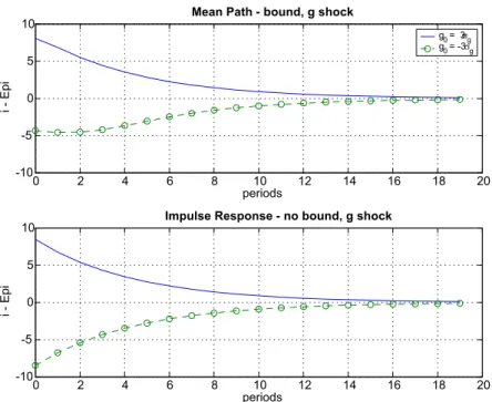
the baseline calibration in table 1.40
Figure 8 illustrates the mean response of the real rate to a ±3 standard deviation real rate shock under optimal policy. The upper panel shows the case with lower bound and the lower panel depicts the case without bound. While in the latter case the policy reaction is perfectly symmetric, imposing the bound creates a sizeable asymmetry: the real rate reduction in response to a negative shock is much weaker than the corresponding increase in response to a positive shock.41
Equation (2), however, implies that the policymaker is unable to affect the average real rate in any stationary equilibrium.42 Therefore, the less
3 9
In this paper we compute welfare losses by taking 1000 random draws of the initial values(u0, g0, µ1
0, µ20) from their stationary distributions under optimal policy (with and without bound) and then evaluate the corresponding welfare losses in the subsequent 1000 periods.
4 0This value is roughly consistent with the estimated variability of real rate shocks in the period 1979:4-1995:2, i.e., the time span considered by Rotemberg and Woodford (1998). The unconditional variance of the real rate shocks for 1979:4-1995:2 is about 2.5-fold that for the period 1983:1-2002:4.
4 1Clearly, this feature emerges because with negative shocks inflation must be used to reduce the real interest rate which is a costly instrument in welfare terms.
4 2This can be seen by taking unconditional expectations of equation (1), imposing sta-tionarity, and noting thatE[gt] = 0.
strong real rate decrease has to be compensated with a less strong real rate increase (or a stronger real rate decrease) in response to other shocks. A close look at figure 8 reveals that this is indeed the case: the real rate increase with the lower bound falls slightly short of the one implemented without bound.
Moreover, it is optimal to undo the asymmetry by trading-off across all shocks, e.g., also across mark-up shocks. This is illustrated in figure 9 which plots the economy’s mean response to±3 standard deviation mark-up shocks. The left-hand panel illustrates the response when the zero lower bound is imposed and the right-hand panel depicts the case without bound. Clearly, the mean reactions change considerably once the lower is imposed. Real rates are now lowered more (increased less) in response to negative (positive) mark-up shocks.
8
Sensitivity Analysis
We now analyze the robustness of our findings by considering a number of variations to our baseline calibration. Particular attention is given to the sensitivity of the results to changes in the parameterization of the shock processes.
8.1
More Variable Shocks
We estimated the shock processes using data for a time period that most economists would consider to be relatively ‘calm’ especially when confronted with the more ‘turbulent’ 1960s and 1970s. Since one cannot exclude that more ‘turbulent’ times might lie ahead, it seems to be of interest to study the implications of optimal policy with more variable mark-up and real rate shocks. In this regard, this section considers the sensitivity of ourfindings to an increase of the shock variancesσu2 andσg2above the values of our baseline parameterization in table 1.
Increasing the variance of mark-up shocks we find that the results are remarkably stable. This holds even when setting the variance ofσu2threefold above its estimated value. Average output and (annual) inflation are slightly positive, but both are yet below 0.01%. Moreover, zero nominal rates occur with the same frequency and persistence as for the baseline parameterization of table 1.
The picture changes somewhat increasing the variance of real rate shocks. While average output remains virtually unaffected, average inflation and the average frequency and persistence of zero nominal rates do change, albeit to different degrees. This is illustrated in figure 10, that depicts the reaction of these variables when the variance of real rate shocks is increased up to threefold above that of the baseline calibration.43 Average inflation and the average persistence of zero nominal rates change only in minor ways. Instead, as real rate shocks become more variable the average frequency of zero nominal rates increases sharply.
Moreover, as can be observed in the lowest panel offigure 10, the average welfare losses generated by the zero lower bound increase markedly with the variance of the real rate shock process. While for the baseline calibration the additional average losses of the zero lower bound over and above those generated by the stickiness of prices is in the order of 1%, once the variance of real rate innovations is threefold the additional losses surge to roughly 33%. This shows that the welfare effects of the zero lower bound are sensitive to the variance of the assumed real rate process.
Note that the effects of the variability of shocks on the average level of output and inflation differ considerably from those reported in earlier contri-butions. Uhlig (2000), e.g., reports negative level effects for both variables when analyzing optimal policy in a backward-looking model. Clearly, the gains from promising positive values of future output and inflation cannot show up in a backward-looking model. Similarly, Orphanides and Wieland (1998) report negative level effects for a forward-looking model considering Taylor-type interest rate rules rather than optimal policy as in this paper. Moreover, unlike suggested by Summers (1991), our results do not show that it is necessary to target positive inflation rates so as to safeguard the economy against hitting the zero lower bound.
8.2
Lower Interest Rate Elasticity of Output
Our benchmark calibration assumes an interest rate elasticity of output of
ϕ= 6.25, which seems to lie on the high side of plausible estimates of the
4 3
This value is roughly consistent with the estimated variability of real rate shocks in the period 1979:4-1995:2, i.e., the time span considered by Rotemberg and Woodford (1998). The unconditional variance of the real rate shocks for 1979:4-1995:2 is about 2.5-fold that for the period 1983:1-2002:4.
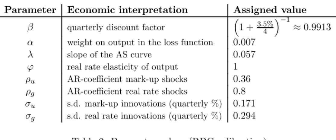
intertemporal elasticity of substitution.44 Therefore, we also consider the case ϕ = 1 that corresponds to log utility in consumption and constitutes the usual benchmark parameterization in the real business cycle literature. Table 2 presents the parameters values implied by table 1 assumingϕ= 1
instead of ϕ= 6.25. Note that the values of λ and α also change as they depend on the intertemporal elasticity of substitution.45
We then re-estimated the shock processes with the new parameter values and using the VAR-predictions to identify expectations. The autocorrelation coefficient for the mark-up shocks now turn out to be statistically significant at the 1% level. Therefore, we setρu equal to its point estimate in table 2.
The point estimate (standard deviation) of the autocorrelation of the real rate shocks is nowρg = 0.882 (0.059). Since we still cannot rejectρg = 0.8at
conventional significance levels, we keep this value. As before, the standard deviationσgis chosen so as to match the standard deviation of the estimated
real rate shocks.
Overall, our findings seem robust to the change in the intertemporal elasticity of substitution. In particular, the level effects on average output and inflation remain negligible. Moreover, required inflation in response to a negative 3 standard deviation real rate shock is still in the order of 15 basis points annually. Even more importantly, the welfare losses generated by the zero bound are rather small and in the order of less than one-half percent of the losses generated by the stickiness of prices alone.
Parameter Economic interpretation Assigned value
β quarterly discount factor
³
1 +3.5%4
´−1
≈0.9913
α weight on output in the loss function 0.007
λ slope of the AS curve 0.057
ϕ real rate elasticity of output 1
ρu AR-coefficient mark-up shocks 0.36
ρg AR-coefficient real rate shocks 0.8
σu s.d. mark-up innovations (quarterly %) 0.171
σg s.d. real rate innovations (quarterly %) 0.294
Table 2: Parameter values (RBC calibration)
4 4As argued by Woodford (2003) this value may capture non-modeled interest-rate-sensitive investment demand.
Respect to the baseline, however, the lower bound is binding more fre-quently, namely in about one quarter every 5 years on average. Binding real rate shocks occur more often because the variance of the real rate shock pro-cess implied by the RBC parameterization is about 45% higher than in our baseline.46 However, binding shocks now generate lower welfare losses: the steeper slope of the Phillips curveλ, shown in table 2, implies that inflation reacts more strongly to output. As a result, the required amount of inflation can be generated with less positive output gaps, which implies lower welfare losses.
9
Conclusions
This paper determines optimal monetary policy under commitment taking directly into account the zero lower bound on nominal interest rates and assesses its quantitative importance for the U.S. economy. One of the main
findings is that, given the historical properties of the estimated shock pro-cesses for the U.S. economy, the zero lower bound seems neither to impose large constraints on optimal monetary policy nor to generate large welfare losses. Furthermore, we show that the existence of the zero lower bound might require to lower nominal interest rates more aggressively in response to adverse shocks than suggested by a model without lower bound.
Ourfindings raise a number of further issues. First, the omission offiscal policy clearly constitutes a shortcoming. The study of the potential role of
fiscal policy in ameliorating adverse welfare effects entailed by the lower bound seems to be of interest. Second, given the widespread belief that lagged inflation is a major determinant of inflation, an issue that should be addressed is the robustness of ourfindings to the introduction of lagged inflation in the Phillips curve.
Finally, the central bank’s credibility is key for our results. The use of expected inflation is unavailable to a discretionary policymaker, as there is no incentive to implement promised inflation ex-post. The zero lower bound on nominal interest rates, therefore, may generate significant welfare losses under discretionary policy, an issue that we explore in a companion paper, Adam and Billi (2003).
4 6
Mark-up shocks also play a less marginal role, a negative shock in the order of 4 standard deviations now leads to a binding lower bound.
10
Appendix
We prove here the claims of proposition 1(REE with Zero Bound)reported in the main text. Let
zt= µ πt yt ¶ , vt= µ ut gt ¶ , m= µ 0 ϕr∗ ¶ and εt= µ εut εgt ¶ .
Forit≡ −r∗ the model is then given by
M0zt=m+M1Etzt+1+vt, (18) where M0 = µ 1 −λ 0 1 ¶ andM1 = µ β 0 ϕ 1 ¶ and vt=Rvt−1+εt with R= µ ρu 0 0 ρg ¶ .
Definingezt≡zt−zwhere the steady state value zis given by
z=
µ
−r∗
−1−λβr∗
one can rewrite (18) as
M0zet=M1Etezt+1+vt (19)
In a REE we have
Etzet+1=zet+1+ηt+1 (20)
where the forecast errorηt+1 is a martingale difference series. Substituting
(20) into (19) delivers the equilibrium law of motion e
zt+1 =Azet−Bvt−ηt+1,
whereA=M1−1M0 and B =M1−1. As is easy verified, A has one unstable
eigenvaluee1> β1 and one stable eigenvalue e2 ∈(0,1).
Now express the forecast errorηt+1 as a combination of the fundamental
innovations and sunspot innovations, i.e.,
where the sunspotsγt+1 are a 2 by 1 martingale difference sequence, while
C and Ddenote arbitrary matrices. We then have e
zt+1 =Azet−Bvt+Cεt+1+Dγt+1. (21)
Since the matrix B has full rank, the shocks vt will put zet on the unstable
subspace of A, even if C and D would restrict εt+1 and γt+1 to lie on
the stable subspace. Since the eigenvector associated with the explosive eigenvalue is of the form
−→e1=µ 1
−e
for somee > 0,yet and πet will diverge into opposite directions. This proves
the existence of a continuum of locally explosive (sunspot) REE.
We now consider stationary solutions. For the reasons discussed above, the only way the solutions (21) can be stationary is if there is a common factor in the lag polynomials that allows to eliminate the termAzet. Rewrite
(21) as
(I−AL)ezt+1 =−Bvt+Cεt+1+Dγt+1
=−Bvt+C(vt+1−Rvt) +Dγt+1
= (I−(B+CR)C−1L)Cvt+1+Dγt+1 (22)
which shows that there is a common factor if A = (B+CR)C−1, that requires
vecC=£(I⊗A)−¡R0⊗I¢¤−1vecB.
The previous equation implies that C = Γ, where Γ is given by equation (15). From (22) it then follows that
e zt+1=Γvt+1+ (I−AL)−1Dγt+1 =Γvt+1+ ∞ X n=0 (AL)nDγt+1. (23)
IfDprojects the sunspotsγon the unstable manifold of Athen these solu-tions are again explosive with yt and πt diverging into opposite directions.
A. The solutions (23) are then stationary. The subspace generated by the eigenvector associated with the stable eigenvalue ofA is
−→e2 = Ã −e2β+ϕλ+β ϕ 1 ! ,
where both entries of−→e2 are positive. The matrix D then has a
represen-tation of the formD=−→e2·(d1, d2)for some constantsd1and d2. Choosing
st = (d1, d2)·γt, φ=e2, w= −e2β+ϕϕλ+β,and applying the definition of ezt
causes (14) and (23) to be equivalent.
References
Adam, Klaus and Roberto M. Billi, “Optimal Monetary Policy under
Discretion with a Zero Bound on Nominal Interest Rates,” University of Frankfurt Mimeo, 2003.
Auerbach, Alan J. and Marurice Obstfeld, “The Case for
Open-Market Purchases in a Liquidity Trap,” NBER Working Paper No. 9814, 2003.
Benhabib, Jess, Stephanie Schmitt-Grohé, and Martín Uribe,
“Avoiding Liquidity Traps,” Journal of Political Economy, 2002, 110, 535—563.
Buiter, Willem H. and Nikolaos Panigirtzoglou, “Overcoming the
Zero Bound on Nominal Interest Rates with Negative Interest on Cur-rency: Gesell’s Solution,”Economic Journal, 2003, 113, 723—746.
Calvo, Guillermo A., “Staggered Contracts in a Utility-Maximizing
Framework,” Journal of Monetary Economics, 1983, 12, 383—398.
Christiano, Lawrence J. and Jonas Fisher, “Algorithms for Solving
Dynamic Models with Occasionally Binding Constraints,” Journal of Economic Dynamic and Control, 2000, 24(8), 1179—1232.
Clarida, Richard, Jordi Galí, and Mark Gertler, “The Science of
Monetary Policy: Evidence and Some Theory,” Journal of Economic Literature, 1999,37, 1661—1707.
, , and , “Monetary Policy Rules and Macroeconomic Sta-bility: Evidence and Some Theory,” Quarterly Journal of Economics, 2000, 115, 147—180.
, , and , “Optimal Monetary Policy in Open versus Closed
Economies: An Integrated Approach,”American Economic Review Pa-pers and Proceedings, 2001, 91, 248—252.
Coenen, Günter and Volker Wieland, “The Zero-Interest-Rate Bound
and the Role of the Exchange Rate for Monetary Policy in Japan,”
Journal of Monetary Economics, 2003, 50, 1071—1101.
Eggertsson, Gauti, “How to Fight Deflation in a Liquidity Trap: Com-mitting to Being Irresponsible,” IMF Working Paper 03/64, 2003.
and Michael Woodford, “Optimal Monetary Policy in a Liquidity
Trap,” NBER Working Paper No. 9968, 2003.
Evans, George and Seppo Honkapohja, “Policy Interaction,
Expecta-tions and the Liquidity Trap,”mimeo, 2003.
Fuhrer, Jeffrey F. and Brian F. Madigan, “Monetary Policy When
Interest Rates Are Bounded at Zero,” Review of Economic Studies, 1997, 79, 573—585.
Giannoni, Marc and Michael Woodford, “Optimal Interest Rate Rules:
I. General Theory,”NBER Working paper No. 9419, 2003.
Goodfriend, Marvin, “Overcoming the Zero Bound on Interest Rate
Pol-icy,”Journal of Money Credit and Banking, 2000,32 (4,2), 1007—1035.
Ireland, Peter, “Technology Shocks in the New Keynesian Model,” 2002. Boston College mimeo.
Judd, Kenneth L., Numerical Methods in Economics, Cambridge: MIT
Press, 1998.
Jung, Taehun, Yuki Teranishi, and Tsutomu Watanabe, “Optimal
Monetary Policy at the Zero-Interest-Rate Bound,” 2001. Hitosubashi University Mimeo.
Kato, Ryo and Shin-Ichi Nishiyama, “Optimal Monetary Policy When
Krugman, Paul R., “It’s Baaack: Japan’s Slump and the Return of the Liquidity Trap,” Brookings Papers on Economic Activity, 1998,49(2), 137—205.
Marcet, Albert and Ramon Marimon, “Recursive Contracts,”
Univer-sitat Pompeu Fabra Working Paper, 1998.
McCallum, Bennett T., “Japanese Monetary Policy, 1991-2001,”Federal
Reserve Bank of Richmond Economic Quarterly, 2003, 89/1.
Miranda, Mario J. and Paul L. Fackler, Applied Computational
Eco-nomics and Finance, Cambridge, Massachusetts: MIT Press, 2002.
Orphanides, Athanasios, “Monetary Policy in Deflation: The Liquidity Trap in History and Practice,” Federal Reserve Board Mimeo, 2003.
and Volker Wieland, “Price Stability and Monetary Policy Eff ec-tiveness When Nominal Interest Rates are Bounded at Zero,” Federal Reserve Board, FEDS Working Paper No. 35, 1998.
and , “Efficient Monetary Policy Design Near Price Stability,”
Journal of the Japanese and International Economies, 2000, 14, 327— 365.
Reifschneider, David and John C. Williams, “Three Lessons for
Mon-etary Policy in a Low-Inflation Era,” Journal of Money Credit and Banking, 2000,32, 936—966.
Rotemberg, Julio J., “The New Keynesian Microfoundations,” NBER
Macroeconomics Annual, 1987,2, 69—104.
and Michael Woodford, “An Optimization-Based Econometric
Model for the Evaluation of Monetary Policy,”NBER Macroeconomics Annual, 1998,12, 297—346.
Schmitt-Grohé, Stephanie and Martín Uribe, “Optimal Fiscal and
Monetary Policy under Sticky Prices,” Journal of Economic Theory (forthcoming), 2003.
and , “Optimal Simple and Implementable Monetary and Fiscal Rules,” Duke University Mimeo, 2003.
Silberberg, Eugene,The Structure of Economics: A Mathematical
Steinsson, Jón, “Optimal Monetary Policy in an Economy with Inflation Persistence,”Journal of Monetary Economics, 2003,50, 1425—1456.
Summers, Lawrence, “Panel Discussion: Price Stability: How Should
Long-Term Monetary Policy Be Determined?,” Journal of Money Credit and Banking, 1991, 23, 625—631.
Svensson, Lars E. O., “Escaping from a Liquidity Trap and Deflation: The Foolproof Way and Others,” Journal of Economic Perspectives (forthcoming), 2003.
Taylor, John B., “Discretion versus Policy Rules in Practice,” Carnegie-Rochester Conference Series on Public Policy, 1993,39, 195—214.
Uhlig, Harald, “Should We Be Afraid of Friedman’s Rule?,” Journal of
Japanese and International Economies, 2000, 14, 261—303.
Wolman, Alexander L., “Real Implications of the Zero Bound on Nominal Interest Rates,” forthcoming Journal of Money Credit and Banking, 2003.
Woodford, Michael, “Doing Without Money: Controlling Inflation in a Post-Monetary World,” Review of Economic Dynamics, 1998, 1, 173— 209.
, “Inflation Stabilization and Welfare,” NBER Working Paper No. 8071, 2001.
-6 -4 -2 0 2 4 84 86 88 90 92 94 96 98 00 02
-.3 -.2 -.1 .0 .1 .2 .3 1 2 3 4 5 6 7 8 Cor(Y,Y(-i)) -.3 -.2 -.1 .0 .1 .2 .3 1 2 3 4 5 6 7 8 Cor(Y,PI(-i)) -.3 -.2 -.1 .0 .1 .2 .3 1 2 3 4 5 6 7 8 C or(Y,I(-i)) -.3 -.2 -.1 .0 .1 .2 .3 1 2 3 4 5 6 7 8 Cor(PI,Y(-i)) -.3 -.2 -.1 .0 .1 .2 .3 1 2 3 4 5 6 7 8 C or(PI,PI(-i)) -.3 -.2 -.1 .0 .1 .2 .3 1 2 3 4 5 6 7 8 C or(PI,I(-i)) -.3 -.2 -.1 .0 .1 .2 .3 1 2 3 4 5 6 7 8 C or(I,Y(-i)) -.3 -.2 -.1 .0 .1 .2 .3 1 2 3 4 5 6 7 8 Cor(I,PI(-i)) -.3 -.2 -.1 .0 .1 .2 .3 1 2 3 4 5 6 7 8 Cor(I,I(-i))
Figure 2: Residual autocorrelations with 2 s.d. error bounds for an unre-stricted VAR in GDP, inflation, and fed funds rate.
-.4 -.3 -.2 -.1 .0 .1 .2 .3 .4 .5 84 86 88 90 92 94 96 98 00 02 -6 -4 -2 0 2 4 6 8 84 86 88 90 92 94 96 98 00 02
u
tg
t-2 -1 0 1 2 -5
0
5 Optimal Policy, u shock
y bound no bound -10 -5 0 5 10 -5 0
5 Optimal Policy, g shock
y -2 -1 0 1 2 -2 0 2 pi -10 -5 0 5 10 -0.1 0 0.1 pi -2 -1 0 1 2 -0.2 0 0.2 i -10 -5 0 5 10 -10 0 10 i -2 -1 0 1 2 -1 0 1 gamma1 -10 -5 0 5 10 -0.04 -0.02 0 0.02 gamma1 -2 -1 0 1 2 -1 0 1 u gamma2 -10 -5 0 5 10 -0.03 -0.02 -0.01 0 g gamma2
-5.5 -5.4 -5.3 -5.2 -5.1 -5 -4.9 -4.8 -4.7 -4.6 -3.6 -3.5 -3.4 -3.3 -3.2 -3.1 -3 -2.9
-2.8 Optimal Policy, g shock
g
i
bound no bound
0 2 4 6 8 10 12 14 16 18 20 -2
0
2 Mean Path - bound, g shock
y g0 = 3σg g0 = -3σg 0 2 4 6 8 10 12 14 16 18 20 -0.2 0 0.2 pi 0 2 4 6 8 10 12 14 16 18 20 -5 0 5 i 0 2 4 6 8 10 12 14 16 18 20 -0.02 0 0.02 gamma1 0 2 4 6 8 10 12 14 16 18 20 -0.02 -0.01 0 gamma2 0 2 4 6 8 10 12 14 16 18 20 -5 0 5 periods i - Epi
1 2 3 4 5 6 7 8 9 10 11 0 0.1 0.2 0.3 0.4 0.5 0.6 0.7 0.8 0.9 Quarters Probability
0 2 4 6 8 10 12 14 16 18 20 -10
-5 0 5
10 Mean Path - bound, g shock
periods i - Epi g0 = 3σg g0 = -3σg 0 2 4 6 8 10 12 14 16 18 20 -10 -5 0 5
10 Impulse Response - no bound, g shock
periods
i - Epi
Figure 8: Asymmetric real rate response with lower bound (3-fold variance of real rate shocks)