Asset Liability Management modeling using
multi-stage mixed-integer Stochastic Programming
Sibrand J. Drijver, Willem K. Klein Haneveld and Maarten H. van der Vlerk∗
September 2000
Abstract
A pension fund has to match the portfolio of long-term liabilities with the portfolio of assets. Key instruments in strategic Asset Liability Management (ALM) are the adjustments of the contribution rate of the sponsor and the reallocation of the investments in several asset classes at various points of time. We formulate a multistage mixed-integer stochastic program to model this ALM process. Special attention is paid to the use of binary variables.
∗ The research of the third author has been made possible by a fellowship of the Royal Netherlands Academy of Arts and Sciences.
1. Introduction
We present a multistage Asset Liability Management (ALM) model based on mixed-integer stochastic programming. Stochastic programming can be used for supporting decision making under uncertainty, while taking into account the probability distri-butions of uncertain parameters. Since it is a powerful tool, stochastic programming is used in many fields, for example in production planning, scheduling problems, location problems and electricity generation (see Birge and Louveaux [1], Kall and Wallace [8], Pr´ekopa [13], Wets and Ziemba [17] and the bibliography Van der Vlerk [16]). It is also used in financial planning models, especially in Asset Liability Management, see for example Boender [2], Cari˜no et al. [3], Consigli and Dempster [4], Dert [5] and Mul-vey and Ziemba [11]. In most of these models, only continuous variables appear. Only Dert uses binary variables in a model with chance constraints. In this paper we show that binary variables can be used to model a variety of realistic features. Next to the chance constraints, binary variables are used to model remedial contributions made by the sponsor of the fund after several periods of underfunding and to model conditional constraints. In addition, we present a flexible modeling of the contribution rate. In this paper we focus on modeling issues. However, the inclusion of integer variables in stochastic programming models causes substantial computational difficulties, see the surveys Klein Haneveld and Van der Vlerk [10] and Stougie and Van der Vlerk [15]. How to deal with these difficulties, for example by using the special structure of the proposed model, will be the subject of our future research.
The contents of this paper can be summarized as follows. In Section 2, we explain what ALM for pension funds is and we also present basic (in)equalities of an ALM model. In Section 3, we propose extensions to these basic (in)equalities, leading to the introduction of binary variables. After modeling the feasible region, we define an ob-jective function. Section 4 shows the dynamic character and the corresponding special structure of the model. In Section 5 we make some concluding remarks.
2. ALM for pension funds
A pension fund has the task of making benefit payments to participants who have ended their active income earning career. We assume that the pension fund has three sources of funding its liabilities: revenues from its asset portfolio, regular contributions made by the sponsor of the fund and remedial contributions made by the sponsor. The latter
payments may be called for if the value of the assets is too low compared to the value of the liabilities. The pension fund has to decide periodically how to distribute the investments over different asset classes and what the contribution rate should be in order to meet all its obligations. This decision process is called Asset Liability Management. A pension fund has long term obligations, up to decades, and therefore its planning horizon is large, too. The main goal of ALM is to find acceptable investment and con-tribution policies that guarantee that thesolvency of the fund is sufficient during the planning horizon. Usually, the solvency is characterized by thefunding ratio Ft, de-fined byFt := At/Lt, whereAt denotes the value of the assets andLt is the value of the liabilities1. The subscripttdenotes timet.Underfunding occurs when the funding ratio is less than one. Another way of characterizing underfunding is by saying that the surplusSt at timet is negative, whereSt :=At −Lt. The funding ratio changes over time, mainly because of uncertain developments in the liabilities and in the returns of the assets. Therefore, a pension fund rebalances its asset portfolio and adjusts its contribution policy regularly, in order to control the funding ratio as well as possible. How much risk of underfunding is acceptable, depends on specific characteristics of the fund. For instance, if the number of active participants is large compared to the number of retired members, some temporary risk of underfunding might be acceptable since there is a possibility to recover later by adjusting the contribution rate if needed. On the other hand, if a limited degree of temporary underfunding is acceptable, this gives the opportunity to increase the investment in stocks and to decrease the investment in bonds. In the long run one may expect that this will increase the returns, since (histor-ically) the mean return on a broadly diversified stock portfolio is higher than that on a broadly diversified bond portfolio; however, its variability is higher too. Of course, if the current funding ratio is much larger than one, there is less reason to worry about promising but risky investments.
In the remainder of this section we describe the basic elements of an ALM model. In order to be realistic we need a dynamic model, since when making decisions at one time, it is necessary to take into account possible adjustments of decisions later, based on observed realizations of uncertain parameters.
1 It is not trivial to calculateLt from the liability portfolio of the fund. We will not go into details on this aspect here.
2.1 ALM model for pension funds: scenarios and decisions
In this section we discuss basic ingredients of an ALM model. Extensions of this model, motivated by the need to incorporate realistic and flexible ways to deal with the risk of underfunding, follow in Section 3.
We split the planning horizon inT subperiods and denote the resulting time stages by an indext. Timet = 0 is the current time andt = T is the length of the horizon. By periodt (t =1, . . . , T ),we mean the span of time[t−1, t). At each timet ∈ T0 :=
{0,1, . . . , T −1}, the pension fund is allowed to make some decisions, for example it may change its asset mix.
One way of modeling uncertainty is through a large but finite number S of scenar-ios. Each scenario represents a possible realization of all uncertain parameters in the model. To be specific, let ωt represent the vector of random parameters whose val-ues are revealed in periodt. Then the set of all scenarios is the set of all realizations
(ωs
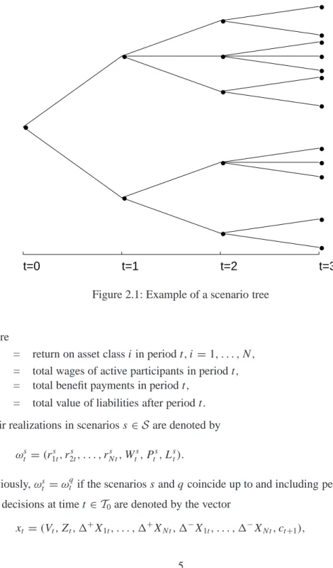
1, . . . , ωsT), s∈S:= {1,2, . . . , S},of(ω1, . . . , ωT). Each scenarioshas a probabil-ityps, whereps >0 andPSs=1ps =1. Since in a dynamic model information on the actual value of the uncertain parameters is revealed in stages, a suitable representation of the set of scenarios is given by a scenario tree, such as in Figure 2.1. In this case,
T =3 andS=12. Each path fromt =0 tot =T represents one scenario. Any node of the tree, corresponding to timet, symbolizes a possible state of the world at time
t, represented by the observed values ofω1, . . . , ωt. The branches directly to the right of it symbolize the various values ofωt+1(and their corresponding conditional proba-bilities) given the realization ofω1, . . . , ωt. Obviously, all scenarios passing this node have the same history in periods 1, . . . , t. The status of the decision variables is related to the scenario tree, too. Basically, a decision at timetmay depend on the observed part of the scenario at that time, but not on unknown values of future periods. That is, for each possible history (i.e. for each node at timetin the scenario tree) there is precisely one vector of decision variables representing the decisions at hand.
However, in our model formulation it is convenient to introduce a complete set of de-cision variables for each scenario separately. Therefore, so-callednonanticipativity or information constraints have to be added, in order to guarantee that decisions do not depend on values of random parameters that will be revealed in later periods.
Let us now introduce the random parameters and the decision variables of the ALM model. Fort ∈T1:= {1,2, . . . , T},we define
• • • • • • • • • •• • •• • • • • • • t=0 t=1 t=2 t=3
Figure 2.1: Example of a scenario tree
where
rit = return on asset classiin periodt, i =1, . . . , N,
Wt = total wages of active participants in periodt,
Pt = total benefit payments in periodt,
Lt = total value of liabilities after periodt. Their realizations in scenarioss∈S are denoted by
ωst =(r1st, r2st, . . . , rNts , Wts, Pts, Lst).
Obviously,ωst =ωtqif the scenariossandq coincide up to and including periodt. The decisions at timet ∈T0are denoted by the vector
where
Vt = restitution to the sponsor at timet,
Zt = remedial contribution by the sponsor at timet,
1+Xit = value of assets in classibought at timet, i=1, . . . , N,
1−Xit = value of assets in classisold at timet, i =1, . . . , N,
ct+1 = contribution rate for periodt+1.
At the time horizont =T, only the decisionsVT andZT occur. The precise meaning of the variables VT andZT will be explained in the next section. Since we introduce decision variables for the same decision in different scenarios, we have the following set of decision variables: fors ∈Sandt∈T0(orT1),
xts =(Vts, Zts, 1+Xs1t, . . . , 1+XsNt, 1−Xs1t, . . . , 1−XNts , cts+1). The corresponding nonanticipativity constraints are, fort∈T0,
xτs =xτq τ =0,1, . . . , t,
for all scenarioss andq that coincide up to time t.
The following additional variables are important too. For each scenarios, and fort ∈
T1:
Ast = total asset value at timet Xs
it = value of investments in asset classi, at the beginning of periodt.
These are state variables (together with Lst). They are determined by the parameters and the decision variables, but from an optimization point of view they are decision variables too, if one includes their definitions as constraints in the model, as we shall do. Next, we have to explain in more detail what we mean by ‘timet’ in the definition ofAst. We assume that at the end of periodt, i.e., just before timet, the contribution of periodtcomes in and the benefit obligations of periodtare paid. At the same time, the revenues of the assets of periodtare revealed. After carrying over a possible restitution to the sponsorVt, or receiving a remedial contribution from the sponsorZt, the total asset valueAs
t is calculated. In Table 1 we give an overview of incoming and outgoing cash flows at timetin scenarios.
Transaction costs, arising from the adjustment of the asset portfolio at time t, do not affectAs
assets at timetin scenariosis given by Ast = N X i=1 (1+rits)Xsit +ctsWts−Pts +Zst −Vts,
fors ∈Sandt ∈ T1. The value of the investments in asset classi, at the beginning of periodt+1 in scenarios, is recursively defined by
Xi,ts +1=(1+rits)Xits −1−Xsit+1+Xsit −ki(1−Xsit +1+Xits), t∈T0, whereki denotes the proportional transaction cost for asset classi. The initial position in each asset classi is given by the parameterXi1(so thatXsi1=Xi1for each scenario
s ∈S). Moreover, all assets should be allocated: N
X i=1
Xi,ts +1 =Ats, s ∈S, t ∈T0.
Realistic scenarios have to satisfy some characteristics. They should for example be consistent with macroeconomic and financial theory. Another aspect is that they should be arbitrage free. That is, it should not be possible to construct a portfolio with zero value such that the payoff in all possible future states is nonnegative and strictly positive in at least one future state.
3. ALM model for pension funds: constraints and objective
In the previous section we defined the scenarios and the decision variables of the model. Now we will introduce a variety of possible constraints and the objective function. Some constraints are already mentioned before: the nonanticipativity constraints and the definitions of the state variables. In addition, nonnegativity is required for the value
incoming cash flows outgoing cash flows
cstWts Pts
PN
i=1ritsXits Vts
Zs t
of each asset classiand for restitutions and remedial contributions
1+Xits ≥0, 1−Xits ≥0, Vts ≥0, Zst ≥0, s ∈S, t ∈T0.
There are also fund-dependent lower and upper bounds for the asset mix:
wli N X j=1 Xsj t ≤Xsit ≤wiu N X j=1 Xsj t s ∈S, t ∈T1,
wherewli and wui are parameters that specify upper and lower bounds on the value of asset classias a fraction of the total asset portfolio.
Moreover, usually policy constraints are included. For instance, upper and lower bounds on the contribution rate are given by
cl ≤cst ≤cu, s ∈S, t ∈T1,
where the numbersclandcuare fund dependent.
The most important constraints, of course, deal with the goal of the pension fund: in all circumstances the funding ratio must be sufficiently high. An obvious way to incorpo-rate this goal in the model, is to add the constraints
Ast ≥αLst, s∈S, t∈T1,
whereα is a policy parameter, usually greater than or equal to one. For example, if
α = 1, the condition asks for nonnegative surplusesSts = Ast −Lst for all scenarios
s ∈Sand timest ∈T1. However, such an implementation might be too strict: it is quite possible that, due to unfavorable developments in the stock market, underfunding is un-avoidable, or that underfunding can only be avoided at unrealistic funding costs. For this reason, we relax these conditions in the next subsections. In the first one, chance constraints are explained. They model so-called Surplus at Risk and some variants of it. Next, we model the possibility of remedial cash flows from or to the sponsor to re-act on a situation of repeated underfunding or overfunding. This is a novelty in ALM modeling; as for chance constraints, binary variables are needed to model it. Similarly, binary variables are used in the third subsection to model the possibility, that certain actions (e.g. taking a position in derivative securities) are allowed, but only in precisely described circumstances. In Section 3.4 flexible goal constraints are formulated with respect to the contribution policy of the pension fund. In the last subsection the ob-jective function is defined: given the constraints, the expected discounted contributions are minimized, together with artificial penalty costs for undesirable decisions such as remedial contributions or rapidly changing contribution rates. We note that the most
important goals of the pension fund are represented in the constraints, as is the case in many other models. The objective function acts as a criterion, which enables the use of optimization algorithms to find a good strategy. Penalty parameters in the objective function do not necessarily have an exact financial interpretation. By varying them, one may try to find feasible solutions that are appreciated by the management of the pension fund.
3.1 Chance constraints
The management of a pension fund wishes to satisfy the goal constraintsAst ≥αLst at all timestand for all scenarioss, for someα ≥1. As explained above, this should not be modeled as a hard constraint. A more realistic model states that the funding ratio in the next period should be sufficiently large with a certain prescribed probabilityφt:
P (Ast ≥αLst)≥φt, t ∈T1. (1) In these chance constraints, the probability distribution used is the conditional distribu-tion ofωtgiven the observed values ofω1, . . . , ωt−1. The value of the parameterφt, the minimum required reliability at timet, is set by the decision makers. It should not be set too low, because then it will lose its meaning of modeling a goal. On the other hand, solving models withφt =1 leads to expensive solutions or to infeasibilities. Also note thatφt may be time dependent. In earlier periods, it may be even less desirable to have a low funding ratio.
In formulation (1), P (Ast ≥ αLst) is called the reliability and 1−P (Ast ≥ αLst) is called the risk of infeasibility. Decisions that are insufficiently reliable (with respect to the next decision moment) are not accepted. This restricts the feasible region.
The above formulation is closely related to Surplus at Risk (SaR). This can be seen as follows. SaR is defined as the estimate of the maximum amount that could be lost in one time period with a prespecified probability due to unfavorable market circumstances. The amount is calculated on the basis of the surplus of the pension fund. Therefore, for any timet the chance constraints in (1) withα =1, describe the condition that the probability that at that time the SaR is negative is at most 1−φt.
In the optimization model, condition (1) acts as a constraint on the decisions at timet, in terms of consequences at timet+1. As a matter of fact, although the representation in (1) does not show this explicitly, there are many chance constraints of this type at time t. Basically, there is a chance constraint for every node in the scenario tree corresponding to timet ∈ T0. Since inequalities (1) cannot be handled directly in a
linear programming framework, they have to be rewritten. This can be done as follows. At timet, we observe the realization ofωt, and therefore know the actual state of affairs
sk
t = (ω1, . . . , ωt). The set of all posible states of affairs at timet will be denoted by
Kt. Definingpt+1(s|stk) as the conditional probability that scenario s occurs at time
t+1 given the state of affairsstk, we can write the chance constraints as S X s=1 pt+1(s|stk)I{Ast+1<αLts+1}(s)≤1−φt, k∈Kt, t∈T0 whereI{Ast<αLst}(s) = 1 if A s
t < αLst and 0 otherwise. Now, we are able to write in-equalities (1) in a mixed-integer linear programming formulation. We introduce binary variablesδ1st, s ∈ S, t ∈ T1. They play the role of shortfall indicators:δ1st must get the value 1 at timet in scenario s if it holds thatAst < αLst, and it must be 0 otherwise. From an optimization point of view, these binary variables are decisions at timet, so they must satisfy the corresponding nonanticipativity constraints. In terms of these ad-ditional decision variables, the chance constraints can be written as linear inequalities:
M1δ1s,t+1≥αLst+1−Ast+1, s ∈S, t ∈T0 (2) S
X s=1
pt+1(s|stk)δ1s,t+1≤1−φt, k∈Kt, t ∈T0. Here,M1is a sufficiently large number.
This formulation was introduced by Dert [5]. He developed a heuristic which first ob-tains a feasible solution of an ALM model satisfying such chance constraints. Next, this solution is improved, while staying feasible. It is not guaranteed, however, that the heuristic finds an optimal solution.
3.2 Remedial contribution after several periods of underfunding
Pension funds want to avoid situations of underfunding, since these are a highly unde-sirable: not all future benefit payments can be guaranteed. One possibility to deal with underfunding is that the sponsor immediately has to pay a remedial contribution, such that the funding ratio is at leastαagain. However, it is quite possible, that such a radical measure is not really necessary. For instance, if there is a quick recovery in the stock market after a correction, it may not be necessary to have a remedial contribution from the sponsor to the fund. If no remedial contribution needs to be paid, the total cost of funding will be reduced.
Instead of requiring a remedial contribution as soon asAst < αLst, we propose to base this decision on the funding ratios of the lastb periods, where b is a natural number chosen by the management of the pension fund or stipulated by the supervisor of the fund. If in at leasta of these periods the funding ratio is less than α, the situation of the pension fund is weak and the sponsor has to pay a remedial contribution to restore the funding ratio. Obviously, a direct payment in case of a funding ratio less thanαis a special case of our more general formulation. Requiring a remedial contribution as soon asAst < αLst is achieved by settinga =b =1. This new modeling is important for at least two reasons. The supervisor of pension funds in the Netherlands seems to judge the solvency position of funds partly on the basis of the chance of underfunding in three successive years ([9]). A second advantage of the above modeling is that it may lead to a lower total cost of funding, which is positive for all active participants, since it may lead to a lower contribution rate.
Next we model the payment of a remedial contribution after several periods of under-funding as mixed-integer restrictions. We introduce binary variablesδs
1t andδ2st,which are used (and needed) to count events. The binary variables in the first inequalities, which are the same as in inequalities (2), indicate whether Fts < α, in which case
δs
1t = 1. The latter inequalities below force δ2st to equal 1 if in the lastb periods the funding ratio is at leastatimes less thanα.
The modeling of remedial contributions as proposed above can be modeled by mixed-integer restrictions as follows:
M1δ1st ≥αLst −Ast bδ2st ≥ t X u=(t−b)++1 δ1su−a+1.
As before,M1is a sufficiently large number, and(x)+:= max{x,0}for everyx ∈R. The sponsor has to pay a remedial contribution ifδ2st =1:
Zts ≥αLst −Ast −M2(1−δs2t), whereM2is a sufficiently large number.
If the sponsor has to pay a remedial contribution at timet, we still count periodt as a period of underfunding(δ1st = 1). Therefore, it is possible that the sponsor has to pay remedial contributions in successive periods. For the time being, we have chosen this formulation, since it is easier to model and – from a practical point of view – it is more
cautious.
If the funding ratio Fs
t is greater than or equal to β, the pension fund may make a restitutionVs
t to the sponsor. In this situation, we can use a reasoning similar to the one given above. Instead of a direct restitution as soon asAst > βLst, the pension fund may make a restitution only after several periods in whichAs
t > βLst. If in these periods the funding ratio falls belowβagain, no restitution will be made. Otherwise it will be made immediately after these periods.
3.3 Conditional constraints
Conditional constraints are of the form: only if a certain event happens, it is allowed to undertake certain actions. To model conditional constraints, binary variables are needed: they take the value 1 if the condition is satisfied and 0 otherwise. The following example illustrates how such conditional constraints can be useful in ALM modeling. From research on returns on stocks and stock indices, Drijver and Otter [7] found that if there is a large negative return in one period, the probability that in the next period there is also a large negative return is statistically greater than would be expected under the assumption that returns are independent and identically distributed.
In an ALM model, this information can be exploited as follows. Since the planning horizon of a pension fund is large, there is usually no reason to consider short-term in-struments, although according to Dert [6], pension funds should invest more in deriva-tive securities. However, if a large drop in returns is observed, it appears to be desirable to allow the fund to take a position in derivative securities, in order to protect the asset portfolio from a further decline.
This extension can be modeled using binary variables in linear constraints. In our ex-ample, the binary variableδ3itequals 1 if and only if a drop of at leastξit×100% occurs in asset classiin periodt.
M3δ3sit ≥(1−ξit)Xi,ts −1−Xits
M4(1−δ3sit)≥Xits −(1−ξit)Xi,ts −1
δ3sit ∈ {0,1}
withM3 and M4 sufficiently large numbers. In that case, a position in derivative se-curitiesDits is allowed (of at most Dimax), which is modeled by the constraintsDits ≤ Dimaxδs
3.4 Flexible modeling of the contribution rate
In the introduction of this section, hard upper and lower boundscl andcuon the con-tribution ratecst were given. Here, we consider a refinement. Not only the level of the contribution rate is important, pension funds (and the sponsor of the fund) also take into account the stability of the contribution rate, since too much variability is undesirable. We can model this as
−ρ≤cts−cst−1≤ρ (3)
for a sufficiently small value ofρ, a parameter to be specified by the decision makers. When the value ofρ is too large, it loses its meaning in modeling a contribution rate which does not change too fast.
On the other hand, if the funding ratio is relatively low for a longer period, it may be better to increase the contribution rate than to ask for remedial contributions for a number of successive periods. This may lead to an increase which is greater thanρ. Hence, it would be better to specify (3) as a goal constraint: changes greater thanρare allowed, but they are penalized in the objective function.
We can model this in a linear programming formulation by the introduction of ad-ditional decision variables cs
t+, representing the amount by which the increase in the contribution rate exceedsρat timet. The second inequality in (3) is replaced by
cst+≥cst −cst−1−ρ
cst+≥0.
In the objective function, we penalize cst+ = (cts −cst−1 −ρ)+, which is positive if
cs
t > cts−1+ρ.
We can use an analogous reasoning in the situation if the funding ratio is relatively high for a number of successive periods. In this situation it may be desirable to lower the contribution rate in two successive periods by more thanρinstead of making resti-tutions to the sponsor in several consecutive periods.
We can model this by the introduction of additional decision variablescst−, representing the amount by which the decrease of the contribution rate in time periodtexceedsρ:
cst−≥cst−1−cts−ρ
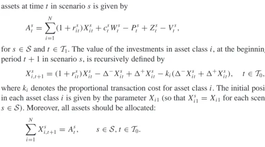
−ρ 0 ρ
(λ+)
(−λ− )
Figure 3.1: Penalization for the change in the contribution rate in two successive peri-ods.
In the objective function, we penalize cs
t− = (cts−1 −cts −ρ)+, which is positive if
cs
t < cts−1−ρ.
We penalizects+andcst−by positive parametersλ+andλ−(usuallyλ−≤λ+), whereas no penalty is imposed if|cs
t−cst−1| ≤ρ. Figure 3.1 shows an example of such a penalty function.
In stochastic programming, this structure, that models piecewise linear increasing costs for shortages and surpluses, is known as multiple simple recourse.
3.5 Objective function
A pension fund wants to minimize the total cost of funding, i.e., the contribution rate for the active participants. Moreover, penalty costs are assigned to the undesirable events discussed above: remedial contributions, large increases and decreases in the contribu-tion rate, and restitucontribu-tions to the sponsor. The latter penalty can also be interpreted as a cost: a lower contribution rate would have been sufficient for a healthy position (in
terms of the funding ratio) of the pension fund.
All these components together constitute the objective function S X s=1 XT t=0 psγts(cstWts +λZZts+λVVts +λ+cst+Wts+λ−cts−Wts) , (4)
whereps is the probability of scenarios,γs
t is the discount factor for a cash flow in pe-riodtin scenarios, andλZ, λV, λ+andλ−are penalty parameters. The definition of the objective function reflects that the pension fund seeks to minimize the total discounted funding costs.
4. Solving the ALM model
We will use stochastic programming to find a good feasible solution of the ALM model described in Sections 2 and 3. The reason is the following. The ALM model is described with linear (in)equalities and a linear objective function. Since stochastic parameters, like returns on the different asset classes, inflation rates and the total wages of the participants, play a crucial role in the ALM model, we need a solution technique that explicitly takes into account these uncertainties. Stochastic programming models are well-suited for our problem, since they allow for progressive revelation of information through time matched by multiple decision stages, where each decision is adapted to the information available at that time. The pension fund will update the portfolio as information about the random parameters becomes available.
Note that, although we are modeling a multistage decision problem, only the first-stage decisions will be implemented. The outcomes of the model for later first-stages are scenario dependent, and therefore not implementable. Moreover, new information be-comes available before decisions on second-stage variables need to be taken. At that time an adapted version of the model is solved; this process is repeated, resulting in a rolling horizon approach.
be written as a (very) large-scale mixed-integer linear program: min S X s=1 ps(d0sx0s +. . .+dTsxTs) s.t. G0x0s =b0 Hs txts−1+Gstxts =bst, s∈S, t ∈T1 Cxt =0, t ∈T0 xs t ∈Xt, s ∈S, t ∈T0. (5)
The objective function in (5) is a reformulation of (4). The matrixG0and vectorb0 de-fine deterministic constraints on the first-stage decisionx0. Fort ∈ T1, Gt, Ht andbt define feasible regions for the recourse decisionsx1s, . . . , xTs. Of course, here the vector
xs
t is larger than has been defined in Section 2: also decision variables that are in-troduced later, such as the binary decision variables, are supposted to be included. The matricesGtandHtand vectorbtmay depend on(ω1, . . . , ωt)but not on(ωt+1, . . . ωT). The equalitiesCxt =0, t ∈T0, wherext = (xt1, . . . , xtS), define the nonanticipativity constraints. Upper and lower bounds on the decision variablesxt, and also integrality restrictions for the binary decision variables, are modeled byXt =Xt(ω1, . . . , ωt), t ∈ T0.
This model embodies the main features of a decision problem under uncertainty. At time t = 0, the decision makers have to select a decision, taking into account fu-ture realizations of the underlying multidimensional stochastic process. Aftert = 0, decisions are allowed to be functions of the observed realization of the stochastic pa-rameters and the past decisions. At each time stage, previous decisions affect current problems through the stochastic matricesHt.
Problem (5) is a large-scale structured mixed-integer linear program. Since the decision makers are faced with uncertainties at each time stage, the number of scenarios (and the number of variables) grows exponentially with the time horizon if in each node the number of successors is at least two. This means that ALM models of realistic size are too large to solve by means of standard solution techniques. It is well known that mixed-integer programming problems are NP-hard (see e.g. [14]); therefore we need to exploit the special structure in (5) even to solve the model approximately.
Because of the size of the problem and the integrality restrictions, the ALM model cannot be solved in reasonable time by standard solution techniques. Therefore, re-search is needed to get a good feasible solution for the ALM model. We will work on this problem and see how for example valid inequalities, Benders decomposition
and (stochastic) branch and bound (see [12]) can be used (in a heuristic) to get a good feasible solution for the ALM model with binary variables.
5. Conclusions
We developed an Asset Liability Management (ALM) model which contains some new and important aspects which we did not encounter in other ALM models, thus allowing more realistic models of the ALM process for pension funds. The first new aspect is the flexible modeling remedial contributions after several periods of underfunding. This new modeling feature is important, since according to Klein Haneveld [9] the superivisor of pension funds in The Netherlands uses this criterion to judge the solvency position of a pension fund.
Also new in ALM modeling is the introduction of conditional constraints. For example, only if a certain drop in the asset portfolio is observed, a position in derivative securities may be taken.
Both modeling issues require the introduction of binary variables. These variables are also needed in modeling chance constraints in a linear programming formulation. We used chance constraints, which are not new in ALM, to impose the condition that the probability of underfunding in the next time period is less than a prespecified parameter. ALM is concerned with making all promised payments at minimum costs. In the ob-jective function these costs appear, together with penalties of undesirable events. Since binary variables appear in the model, it is very difficult to obtain even a feasible solution for ALM models of realistic size. In future research we will try to obtain a good feasible solution for the multistage mixed-integer stochastic program.
References
[1] J.R. Birge and F. Louveaux. Introduction to Stochastic Programming, Springer-Verlag, New York, 1997.
[2] C.G.E. Boender. A hybrid simulation/optimisation Scenario Model for Asset Lia-bility Management. European Journal of Operations Research, 99: 126-135, 1997. [3] D.R. Cari˜no, T. Kent, D.H. Myers, C. Stacy, M. Sylvanus, A. Turner, K. Watanabe and W.T. Ziemba. The Russell-Yasuda Kasai financial planning model. Interfaces, 24:29-49, 1994.
[4] G. Consigli, M.A.H. Dempster. Dynamic Stochastic Programming for Asset Lia-bility Management, Annals of Operations Research, 81: 131-162, 1998.
[5] C.L. Dert. Asset Liability Management for Pension Funds: A Multistage Chance Constrained Programming Approach, Ph.D. thesis, Erasmus University Rotter-dam, 1995.
[6] C.L. Dert. Wie niet waagt, die wint. Over opties en gemiste kansen. (inaugural lecture), Vrije Universiteit Amsterdam, 1999.
[7] S.J. Drijver and P.W. Otter. On rebalancing a Sector Portfolio Model based on Predictions of Sector Returns and Markov Chains.
[8] P. Kall and S.W. Wallace. Stochastic Programming, Wiley, Chichester etc.,1994. [9] H.A. Klein Haneveld. Solvabiliteitscriteria voor pensioenfondsen, Ph.D. thesis,
University of Groningen, 1999.
[10] W.K. Klein Haneveld and M.H. van der Vlerk. Stochastic Integer Programming: General models and algorithms, Annals of Operations Research, 85: 39-57, 1999. [11] J.M. Mulvey and W.T. Ziemba (editors). Worldwide Asset and Liability
Model-ing. Cambridge University Press, 1998.
[12] V.I. Norkin, G.C. Pflug and A. Ruszczy´nski. A branch and bound method for stochastic global optimization. Mathematical Programming, 83(3,Ser. A): 425-450,1998.
[13] A. Pr´ekopa. Stochastic Programming, Kluwer Academic Publishers, 1994. [14] A. Schrijver. Theory of Linear and Integer Programming. Wiley, 1986.
[15] L. Stougie and M.H. van der Vlerk. Stochastic integer programming. In M. Dell’Amico, F. Maffioli, and S. Martello, editors, Annotated Bibliographies in Combinatorial Optimization, chapter 9, pages 127-141. Wiley, 1997.
[16] M.H. van der Vlerk. Stochastic programming bibliography. World Wide Web, http://mally.eco.rug.nl/biblio/stoprog.html, 1996-2000.
[17] R.J.-B. Wets and W.T. Ziemba. Stochastic Programming: State of the Art 1998. Annals of Operations Research, to appear.