Dimitri Marinakis, Philippe Gigu`ere, and Gregory Dudek Centre for Intelligent Machines, McGill University, 3480 University St, Montreal, Quebec, Canada H3A 2A7
{dmarinak,philg,dudek}@cim.mcgill.ca http://www.cim.mcgill.ca
Abstract. In this paper, we present an approach for recovering a topological map
of the environment using only detection events from a deployed sensor network. Unlike other solutions to this problem, our technique operates on timestamp free observational data; i.e. no timing information is exploited by our algorithm except the ordering. We first give a theoretical analysis of this version of the problem, and then we show that by considering a sliding window over the observations, the problem can be re-formulated as a version of set-covering. We present two heuristics based on this set-covering formulation and evaluate them with numer-ical simulations. The experiments demonstrate that promising results can be ob-tained using a greedy algorithm.
Key words: sensor networks, topology inference, set-covering, mapping
1
Introduction
In this paper we consider the problem of learning the topology of a network of sensors through the exploitation of motion in the environment. We assume that an individual sensor is capable of detecting the passage of an agent through its local region, but is un-able to generate a reliun-able signature. Our approach uses the combined observational data returned from our network to infer the topological relationships between the sensors.
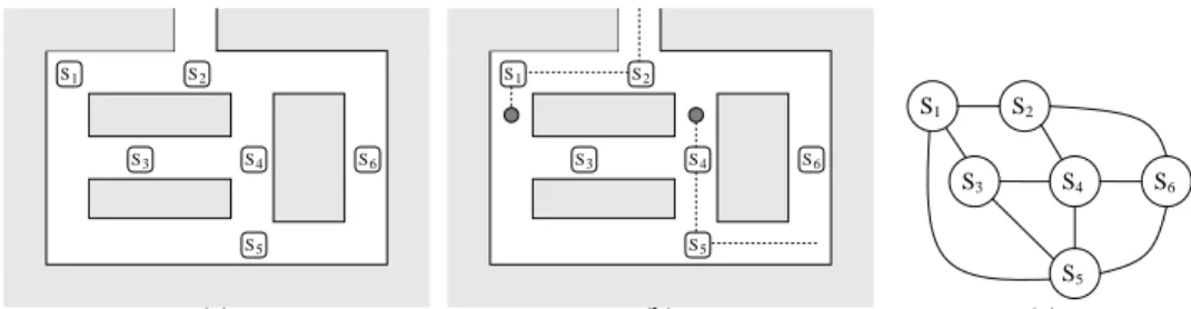
We will illustrate the problem with a simplified example. Figure 1(a) depicts a sen-sor network distributed within an indoor environment. Let us assume that the network has been deployed for some purpose, such as surveillance, and requires knowledge of the inter-node connectivity in order to fulfill its function. During some initial calibration period the network collects observations of agents passing by each sensor (Figure 1(b)). The problem we are trying to solve is how to use these collected observations to con-struct the topological description of the network shown in Figure 1(c). This type of network might arise if wireless cameras were deployed in a workplace environment.
In this work, we assume not only that the agents moving though the environment are indistinguishable, but that there are no temporal clues that can be used to aid the inference process. In other words, the detection events are correctly ordered but are not
time-stamped. Therefore, when our inference algorithm is employed, the time-stamp
data can be discarded or simply not collected in the first place. In order to exploit timing information in the observational sequence some model of agent motion in the environ-ment needs to be either constructed based on prior assumptions, or learned from the
S1 S2 S3 S4 S6 S5 (a) S1 S2 S3 S4 S6 S5 (b) S1 S3 S5 S4 S6 S2 (c)
Fig. 1. An example of a sensor network which we wish to calibrate. a) The original ad-hoc
de-ployment. b) An Example of agent motion exploited by the calibration process. c) The desired topological connectivity map of the network.
data. Our technique, however, allows the correct edges in the graph to be inferred while avoiding the prior domain knowledge or algorithmic complications involved in con-structing an adequately accurate motion model. By employing a sliding window over the observations, we will show that the problem can be re-formulated as a version of the well understood set-covering problem and accurate results can be obtained without timing information.
The ability of a surveillance or monitoring system to automatically determine the connectivity parameters describing its environment is useful for a number of reasons. Although the topology information can be manually entered during installation, more detailed parameters such as the relative connectivity strength between links are difficult to determine, and a change in the environment or network would require re-calibration. Once calibrated, the connectivity information could aid in conventional target track-ing and additional monitortrack-ing activities. For example, by reconstructtrack-ing trajectories, a vehicle monitoring network distributed about a city could help make decisions about road improvements which might best alleviate congestion. In addition, the topological information could be combined with relative localization techniques [1] [2] [3] [4] to recover a more complete representation of the environment.
2
Background
Although the topological mapping problem has been well explored in mobile robotics [5] [6] [7] [8], most sensor network related investigations have been more recent [9] [10] [11] [12]. The outcome is generally a graph where vertices represent embedded sensors in the region and edges indicate navigability.
Ellis, Markis, and Black [9] approached the topology inference problem in the con-text of camera-based sensing. Their technique exploits temporal correlations in obser-vations of agents’ movements. They outlined an approach in which they first identified entrance and exit points in camera fields of view to generate a graph from video data. They then used a thresholding technique to look for peaks in the temporal distribution of travel times between entrance-exit pairs; a clear peak suggesting that the cameras
are linked. This approach requires a large number of observations, but does not rely on object correlation across specific cameras. Thus, the method can be used to efficiently produce an approximate network connectivity graph.
Marinakis and Dudek [11] [12] have recently presented a solution to the topological inference problem that is based on a stochastic version of the Expectation Maximiza-tion algorithm. Their approach uses only detecMaximiza-tion events from the deployed sensors and is based on reconstructing plausible agents trajectories. Results presented from simula-tions and experimental data suggest that their technique produces accurate results under a variety of conditions and compares well to other approaches.
When the observation are information-poor, topology inference through trajectory reconstruction has much in common with the data association problem in multi-object tracking and similar statistical techniques are employed. For example, in [13], event detections alone were used for the tracking of multiple targets using Markov Chain Monte Carlo (MCMC). Similarly, [14] approached a traffic monitoring problem using limited sensor data observations through a stochastic sampling approach.
A key observation regarding all of the approaches mentioned above is that their performance will suffer if temporal information is removed from the observations. Ellis, Markis, and Black rely explicitly on this temporal data, while the approaches employing probabilistic frameworks [11] [13] [14] exploit the delay information to aid in the data association problem.
In the remainder of this paper, we consider the problem of solving the topology inference problem, relying only on the ordering of the timing information in the obser-vational data. We discuss theoretical aspects of this version of the problem and present an algorithm for its solution. It is our hope that concepts presented here can be incorpo-rated into more general techniques for topology inference, or used in their own right.
3
Problem Definition
We formulate the problem of learning the network topology as the inference of a di-rected graphG = (V, E), where the verticesV = vi represent the locations where
sensors are deployed, and the edgesE=ei,jrepresent the connectivity between them;
an edgeei,jdenotes a path from the position of sensorvito the position of sensorvj.
The sources of motion in the sensor network are modeled as some numberN of agents moving asynchronously through the graph. Each agent generates an observation every time it visits a vertex. This corresponds to an agent passing near a particular sensor which then detects the presence of motion in its region.
The input to the problem is an ordered list of observationsO={ot}, each of which
is identifiably generated by one of the sensors; i.e. eachot∈[1, V]. The goal is to find
4
Algorithm Formulation
4.1 Smallest Graph is Correct Answer
The key idea behind our approach is to find the smallest1 graph that successfully ex-plains the observed data. Leaving aside for the moment the actual implementation de-tails, let us consider this idea in more depth by proposing the existence of an algorithm
A that takes as an input the assumed number of agentsN′ in the environment and the
observational sequence and returns as an output the smallest graph consistent with the observations.
Our algorithm A considers each of the possible trajectories that could be taken by theseN′agents given the observational sequence and then selects the trajectory set that
requires the smallest number of inter-vertex traversals. The algorithm then returns the graph populated only with edges that correspond to the inter-vertex traversals required by this chosen trajectory set.
The concept that the simplest solution explaining the data is probably the correct solution has been used successfully in a different version of the topology inference problem [12]. The principle, known as Occam’s razor, states, “if presented with a choice between indifferent alternatives, then one ought to select the simplest one.” The concept is a common theme in computer science and underlies a number of approaches in AI;
e.g. hypothesis selection in decision trees and Bayesian classifiers [15]. We will show in
the next section that under certain assumptions, we can prove that an algorithm trying to find the smallest graph will return the correct answer.
4.2 Correctness of the Smallest Graph Assumption
In this section we present a proof that the smallest graphGconsistent with the obser-vations is the correct solutionGcgiven the following assumptions:
1. There are an infinite number of observations,O. 2. The motion of each of the agents is random.
3. The true number of agents in the systemN is fixed and bounded by the number assumed by the algorithm A; i.e.N <=N′.
4. The transit time between nodes is un-bounded.
5. There are no self-referential connections in the true graphGc; i.e. no agent may
trigger two observations by one passage through the region of a single sensor.
4.3 Proof of Smallest Graph
First, we will prove that there exist no graph smaller thanGc that can explain the
ob-served data, given the above stated assumptions. This is done by showing that it is possible to have sequences generated byGc that cannot be explained by this smaller
graphG′
c. In other words,G′cis not consistent with the observations, and by definition
cannot be a solution.
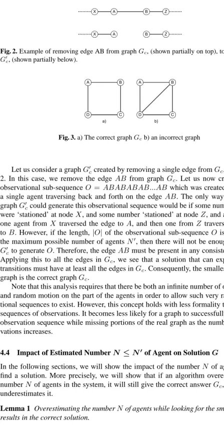
Fig. 2. Example of removing edge AB from graphGc, (shown partially on top), to create graph
G′
c, (shown partially below).
Fig. 3. a) The correct graphGcb) an incorrect graph
Let us consider a graphG′
ccreated by removing a single edge fromGc, as in figure
2. In this case, we remove the edge AB from graph Gc. Let us now create a valid
observational sub-sequenceO =ABABABAB...ABwhich was created in truth by a single agent traversing back and forth on the edgeAB. The only way agents in a graphG′
ccould generate this observational sequence would be if some number of them
were ‘stationed’ at nodeX, and some number ‘stationed’ at nodeZ, and alternatively one agent fromX traversed the edge to A, and then one fromZ traversed the edge toB. However, if the length,|O|of the observational sub-sequenceO is larger than the maximum possible number of agentsN′, then there will not be enough agents in
G′
cto generateO. Therefore, the edgeABmust be present in any consistent solution.
Applying this to all the edges in Gc, we see that a solution that can explain all the
transitions must have at least all the edges inGc. Consequently, the smallest consistent
graph is the correct graphGc.
Note that this analysis requires that there be both an infinite number of observations and random motion on the part of the agents in order to allow such very rare observa-tional sequences to exist. However, this concept holds with less formality to very large sequences of observations. It becomes less likely for a graph to successfully explain an observation sequence while missing portions of the real graph as the number of obser-vations increases.
4.4 Impact of Estimated NumberN ≤ N′of Agent on SolutionG
In the following sections, we will show the impact of the numberN of agent used to find a solution. More precisely, we will show that if an algorithm overestimates the numberN of agents in the system, it will still give the correct answerGc, but not if it
underestimates it.
Lemma 1 Overestimating the numberNof agents while looking for the smallest graph results in the correct solution.
To prove this lemma, we will show that a path generated by a single agent can be spliced between two agents using a ‘tag team’ method, and yet will still a yield a the correct graphGc. That way, all superflouous agents used in the algorithm can be
‘hidden’ by splicing a valid path repeatedly.
Let us consider a true sequence of vertex traversalsSgenerated by a single agent. First, without loss of generality, select any vertexvsplice ∈ S as a splicing node. We
can now pair any two virtual agents together to generate this traversal sequenceS in the following way. Let one of the virtual agent be initially stationed atvsplice. When
the other virtual agent enters this vertex it will exchange its role with the first agent, as in a game of tag team wrestling. The other agent will now leave the vertexvsplice,
generating a sub-sequence ofSuntil it re-entersvsplice, where again they will switch
roles.
As an example, let us consider the vertex sequenceS =ABCDADCDABCBA
generated by a true agent in Gc of Figure 3(a.). We choose vsplice = C. Now the
vertex sequence S assumed to come from a single agent looks like the following:
ABcdadCDABcbawhere capital letters are used for the pathP1 of agent one, and small bold letters are used for the pathP2of agent two. The individual virtual sequences
P1 = ABCDABandP2 =cdadcbaare both valid sequences in the correct graph
Gc.
This analysis shows that we can assume the existence of more agents than the num-ber that actually generated the observation sequence, and still produce paths that are consistent with the correct graph.
Lemma 2 Underestimating the number of agents can result in an incorrect solution. To prove this lemma, we will simply show that there exists at least one observational sequenceOsuch that underestimating the number of agents creates a false solution. Let us consider again the graph depicted in figure 3(a.) and let us consider the motion of two agents in this graph. Agent one will follow the pathABCDADC, and agent two will follow the path db. By combining the two paths, it is possible to get the sequence of observations:O1=ABdCDAbDC. If we assumed the existence of only one agent,
then the smallest graph that can explain the transitionsO1 is displayed in figure 3(b.)
and is incorrect.
Using the above stated two lemma, we arrive at the following theorem (which holds true given the earlier stated assumptions):
Theorem 1 If the number of assumed agentsN′ in the algorithm is equal or greater
than the true number of agents N that generated the observations, then the smallest
graph consistent with the observations will be the correct graphGc. If the number of
assumed agent is smaller than the true number, then there are no guarantees that the
smallest graph consistent with the observations will be the correct graphGc.
In the next section, we draw on this theoretical analysis to motivate a pragmatic approach for topology inference.
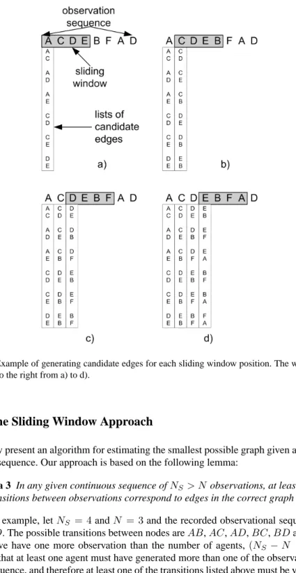
Fig. 4. Example of generating candidate edges for each sliding window position. The window is
moved to the right from a) to d).
5
The Sliding Window Approach
We now present an algorithm for estimating the smallest possible graph given an obser-vation sequence. Our approach is based on the following lemma:
Lemma 3 In any given continuous sequence ofNS > Nobservations, at least(NS−
N)transitions between observations correspond to edges in the correct graphGc.
For example, letNS = 4andN = 3and the recorded observational sequence be
ABCD. The possible transitions between nodes areAB,AC,AD,BC,BDandCD. Since we have one more observation than the number of agents,(NS −N = 1), it
means that at least one agent must have generated more than one of the observations in this sequence, and therefore at least one of the transitions listed above must be valid; i.e.
present inGc. Note that the number of potential transitions generated with a sequence
ofNS observations is:
NT =
(NS−1)NS
2
Our technique is to employ a sliding window of sizeNS = N+ 1to consider in
turn small continuous subsequences of the entire observation sequenceO. Each of these subsequences gives rise to a list ofNT = (N2+N)/2candidate edgesLi, one of which
must be present in the true solutionGc. Once the window has moved over the complete
observation sequenceO, there will beK=|O| −NSlists generated. Figure 4 shows an
example of generating candidate edges using the sliding window approach. Motivated by Theorem 1, our approach is find the smallest graph that can explain at least one edge in each in each of these candidate lists:L1, L2, ...LK.
This problem can be shown to be equivalent to the set-covering problem which is NP-complete, however, several heuristics can be employed to estimate an optimal solution. We will consider a two heuristic approaches in the next sections.
5.1 A Greedy Approach
One method of obtaining a solution to the sliding window problem posed above, is to adopt a greedy approach. This is a standard heuristic often used with good results for set-covering problems. In our domain, the greedy algorithm would work as follows:
1. Begin by marking all candidate listsL1, L2, ...LKunexplained and initialize a list
of edgesEto be empty.
2. Find the edge e that is present in the greatest number of currently unexplained candidate lists.
3. Remove from consideration those candidate lists which contain edgeeby marking them explained, and addetoE.
4. Repeat steps 2 to 3 until all lists are marked explained. Return the graph corre-sponding to our list of edgesEas the final solution.
5.2 A Statistical Approach
A statistical approach could also be used to determine the correct edges in Gc. The
number of times a given edge has been seen in any candidate list could be tallied up. Those edges that occur with a frequency greater than some thresholdT could then be selected.
Let us consider a suitable value for the thresholdT. IfGc corresponded to a fully
connected undirected graph, the average tally of each edge would be:
µ=KNT |E|
whereNT is the number of candidate edges generated per window,Kis the number
of candidate lists (windows), and |E|is the number of potential edges in the graph. ReplacingKwith|O| −NS,NT with(N2+N)/2, and|E|withV(V −1), we arrive
(a) (b)
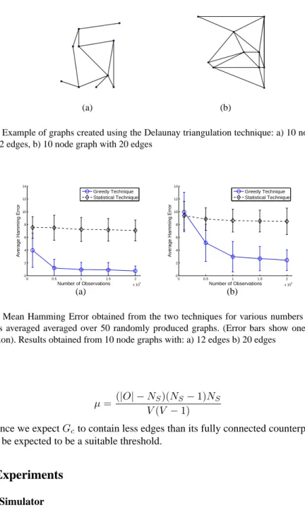
Fig. 5. Example of graphs created using the Delaunay triangulation technique: a) 10 node graph
with 12 edges, b) 10 node graph with 20 edges
0 0.5 1 1.5 2 x 10⁴ 0 2 4 6 8 10 12 14 Number of Observations
Average Hamming Error
Greedy Technique Statistical Technique (a) 0 0.5 1 1.5 2 x 10⁴ 0 2 4 6 8 10 12 14 Number of Observations
Average Hamming Error
Greedy Technique Statistical Technique
(b)
Fig. 6. Mean Hamming Error obtained from the two techniques for various numbers of
obser-vations averaged averaged over 50 randomly produced graphs. (Error bars show one standard deviation). Results obtained from 10 node graphs with: a) 12 edges b) 20 edges
µ=(|O| −NS)(NS−1)NS
V(V −1)
Since we expectGcto contain less edges than its fully connected counterpart,T =
µcan be expected to be a suitable threshold.
6
Experiments
6.1 Simulator
We have examined the sliding window approach with a number of experiments con-ducted in simulation. We have constructed a simulation tool that takes as input a graph and the number of agents in the environment and outputs a list of observations generated by randomly walking the agents through the environment. A number of experiments were run using this simulator on randomly generated planar, connected graphs (Figure
1 2 3 4 5 6 7 0 5 10 15 20 25 30 35
Assumed Number of Agents
Average Hamming Error
True Number of Agents (a) 0 0.5 1 1.5 2 x 10⁴ 0 1 2 3 4 5 6 Number of Observations
Average Hamming Error
Accurate Assumption Over−estimate
(b)
Fig. 7. Results obtained by differing the assumed number of agents for graphs of size 10 nodes
and 14 edges. a.) Hamming Error as a function of the assumed number of agents for the greedy algorithm. Results obtained with 10000 observations generated from 4 agents and averaged over 10 graphs. (Error bars show one standard deviation). b.) Mean Hamming Error as a function of observations for an accurate assumption of 4 agents and an over-estimate of 5 agents. Results averaged over 50 graphs.
5). The graphs were produced by selecting a connected sub-graph of the Delaunay tri-angulation of a set of randomly distributed points. For each experiment, the results were obtained by considering the Hamming error between the true and inferred graph.
6.2 Results
The greedy approach was capable of producing accurate results in moderately sized graphs with a reasonable number of agents, given an adequate number of observations. Although not as accurate on average as the greedy approach, the statistical approach was also capable of producing a solution near the true answer. Figure 6 compares the accu-racy of theses two approaches over 50 randomly produced graphs of 10 nodes and two different edge densities. Note that the accuracy of both approaches tended to increase as the number of observations increased. It also appeared that denser graphs required larger numbers of observations to obtain the same accuracy level than that obtained in sparser graphs. Additionally, it was observed that the greedy approach obtained a better Hamming error on average for less dense graphs. However, when the proportion of the true graph structure recovered was considered, this effect was lessened. For example, for the experiment shown in figure 6, the Hamming error divided by the true number of edges in the graph was approximately double for denser graph, while the Hamming error alone was approximately triple.
Unsurprisingly, the accuracy of the statistical approach was very sensitive to the value of the threshold selected. Experiments not shown here verified that the value forT
selected above was generally suitable for graphs of various densities and sizes, although often better results could be obtained for any specific graph type through careful tuning. This approach requires relatively little computational effort and might have value as a bootstrapping technique for more complex approaches such as the one presented in [11].
1 2 3 4 5 6 7 0 1 2 3 4 5 6 7 8
True Number of Agents
Average Hamming Error
(a) 1.5 2 2.5 3 3.5 4 4.5 5 5.5 6 6.5 0 0.5 1 1.5 2 2.5x 10 4
Number of Observations Needed
True Number of Agents
(b)
Fig. 8. Performance of algorithm as a function of the true number of agents for the greedy
algo-rithm where the assumed number of agents is set to the correct number. Results averaged over 10 graphs of size 10 nodes and 14 edges; (error bars show one standard deviation). a.) Hamming Error obtained with 10000 observations. b.) Number of observations required to obtain a result with a Hamming error of 2 or less.
As predicted by theorem 1, the effect of over-estimating the number of agents in the environment was indeed less detrimental than that of under-estimating the number of agents. Figure 7 shows the result of assuming various numbers of agents in one situation for the greedy approach. As the over-estimation increases, the required number of observations needed to solve the problem also increases.
The problem of topology inference becomes more difficult as more agents are added to the system. Figure 8 shows the correspondingly poorer performance obtained with the greedy approach on the same set of graphs with observations generated from dif-ferent numbers of agents. Even if the correct number of agents is known, we suspect that less information is available as the number of agents increases. As the size of the sliding window increases, so does the number of candidate edges generated by each sliding window. Therefore, the ratio of known correct to incorrect edges decreases, and hence, more observations are needed to obtain the same level of error.
7
Conclusion
In this paper, we have described a way of learning the topology of a sensor network, using only event ordering information. We presented a theoretical analysis of the prob-lem, and re-formulated it as a set-covering problem. Two methods were presented to solve this problem, one based on statistics, and one based on a sliding window tech-nique. We explored the effectiveness of both approaches through numerical simulations for various test cases. Our work demonstrates the promise of this approach for topology inference.
In future work, we hope to extend some of our theoretical results. We would be interested in furthering our understanding regarding the impact of the number of agents in the system since this value tends to dilute the information gained per each observa-tion. This effort would entail deriving a relationship for the information gained in the
context of the sliding window approach. Additionally, it would be of interest to find an analytical relationship between the number of observations needed to solve a problem and the corresponding density of agents in the system; i.e. the ratio of agents to edges in the true graph. On a different level, we would like to apply the findings presented in this paper to the version of the problem where timing data is available and compare it to other established methods.
Acknowledgments. We would like to acknowledge Ketan Dalal for his helpful analysis of this problem.
References
1. Savvides, A., Han, C., Strivastava, M.: Dynamic fine-grained localization in ad-hoc networks of sensors. In: 7th annual international conference on Mobile computing and networking, Rome, Italy (2001) 166–179
2. Moore, D., Leonard, J., Rus, D., Teller, S.: Robust distributed network localization with noisy range measurements. In: Proc. of the Second ACM Conference on Embedded Networked Sensor Systems (SenSys ’04), Baltimore (2004)
3. Marinakis, D., Dudek, G.: Probabilistic self-localization for sensor networks. In: AAAI National Conference on Artificial Intelligence, Boston, Massachusetts (2006)
4. Ihler, A.T., Fisher III, J.W., Moses, R.L., Willsky, A.S.: Nonparametric belief propagation for self-calibration in sensor networks. IEEE Journal of Selected Areas in Communication (2005)
5. Shatkay, H., Kaelbling, L.P.: Learning topological maps with weak local odometric infor-mation. In: IJCAI97, San Mateo, CA (1997) 920–929
6. Choset, H., Nagatani, K.: Topological simultaneous localization and mapping (SLAM): to-ward exact localization without explicit localization. IEEE Transactions on Robotics and Automation 17(2) (2001) 125 – 137
7. Remolina, E., Kuipers, B.: Towards a general theory of topological maps. Artif. Intell. 152(1) (2004) 47–104
8. Ranganathan, A., Dellaert, F.: Data driven MCMC for appearance-based topological map-ping. In: Proceedings of Robotics: Science and Systems, Cambridge, USA (2005)
9. Makris, D., Ellis, T., Black, J.: Bridging the gaps between cameras. In: IEEE Conference on Computer Vision and Pattern Recognition CVPR 2004, Washington DC (2004)
10. Rekleitis, I., Meger, D., Dudek, G.: Simultaneous planning localization, and mapping in a camera sensor network. Robotics and Autonomous Systems (RAS) Journal, special issue on Planning and Uncertainty in Robotics (2006)
11. Marinakis, D., Dudek, G.: A practical algorithm for network topology inference. In: IEEE Intl. Conf. on Robotics and Automation, Orlando, Florida (2006)
12. Marinakis, D., Dudek, G.: Topological mapping through distributed, passive sensors. In: International Joint Conference on Artificial Intelligence, Hyderabad, India (2007)
13. Songhwai Oh, Phoebus Chen, M.M., Sastry, S.: Instrumenting wireless sensor networks for real-time surveillance. In: Proc. of the International Conference on Robotics and Automa-tion. (2006)
14. Pasula, H., Russell, S., Ostland, M., Ritov, Y.: Tracking many objects with many sensors. In: IJCAI-99, Stockholm (1999)