Ashdown Forest visitor survey data analysis

(1)

Natural England Commissioned Report NECR048

Ashdown Forest visitor survey

data analysis

(2)

(3)

Foreword

Natural England commission a range of reports from external contractors to

provide evidence and advice to assist us in delivering our duties. The views in this

report are those of the authors and do not necessarily represent those of Natural

England.

Woodlark

Background

Natural England is the Government’s advisor on nature conservation and has specific statutory roles with regards to European sites such as the Ashdown Forest Special Protection Area (SPA). The visitor surveys were undertaken on behalf of the two local planning authorities as part of their Habitats

Regulations Assessment of their Core Strategy and in particular their housing allocations. Natural England are encouraging all planning authorities whose strategies could increase recreational

pressures on sensitive European sites such as those with ground nesting birds to undertake appropriate visitor surveys. One of Natural England’s key roles is to help Local Planning Authorities (LPAs) and owners of special sites understand how their work and plans could affect SPAs and to help them devise how any negative impacts can be ameliorated. This report was commissioned by Natural England to help the LPAs, owners and visitors to Ashdown Forest understand the existing and potential future impacts of visitors on

the SPA birds and to encourage approaches and behaviour which ameliorates or even prevents those impacts.

The LPA will devise and implement the mitigation strategy in terms of Development Control and LDF policies. Natural England are working with the LPA, owners and managers of the SPA to develop a clear visitor management approach which includes elements of on-SPA mitigation. Natural England are involved in the national monitoring strategies for the SPA birds but we will also be working with the owners of the site, the LPA and others to encourage more detailed monitoring of the birds.

This report should be cited as:

CLARKE, R. T., SHARP, J. & LILEY, D. 2010.

Ashdown Forest visitor survey data analysis. Natural England Commissioned Reports, Number 048.

Natural England Project Manager - Louise Bardsley, Government Team (Eastern Area Team), Lewes Office, Phoenix House, 33 North Street, Lewes BN72PH [email protected]

Contractor - Joanna Sharp and Durwyn Liley Footprint Ecology, Ralph Clarke Bournemouth University

Keywords - access, analysis, Ashdown Forest, breeding birds, development, disturbance, habitats regulations, heathlands, housing, spatial planning, special areas of conservation (sac), special protection areas (spa), survey, visitor pressure

Further information

This report can be downloaded from the Natural England website: www.naturalengland.org.uk. For

(4)

(5)

Summary

This report relates to Ashdown Forest, which is classified as a Special Protection Area (SPA) due to the presence of breeding nightjars and Dartford warblers and a Special Area of Conservation (SAC) due to the heathland habitats present on the site. The protected site forms a contiguous block of heathland and wooded habitats of around 3000ha. The Forest is close to existing settlements such as Crawley, East Grinstead, Crowborough and Tunbridge Wells. This report has been commissioned by Natural England to consider in detail current visitor rates to the site and the distribution of birds within the site in relation to visitor pressure. Such information and analysis is necessary to guide spatial planning in the area.

We use data collected originally by UE Associates in September 2008, a visitor survey that involved visitor questionnaires and counts of people at 20 of the access points within Ashdown Forest. Within this survey data (a total of 645 interviews), 343 (53%) of the interviewed people provided full, valid

postcodes, which enables us to determine the (GIS straight-line) distance from their home postcode to the access point where they were interviewed. These geocoded data show that 15% of interviews were conducted with visitors who lived less than 1km away from the location where they were interviewed, 50% within 5km and 90% within 17km.

There are a total of 78 access points at Ashdown Forest. In order to predict total visitor numbers to Ashdown Forest it is necessary to derive estimates for the unsurveyed access points. To do this we treat visitors arriving on foot and by car separately and use data on the car-park capacity at each access point and the number of houses at different distance bands away from each access point (extracted from a postcode database within the GIS). People arriving from foot live close to the site and visit rate

declines with distance such that no people travelling on foot were recorded visiting from beyond 1500m. The visitor rate for pedestrians declined with distance such that for people within 500m the number of visits (per person per 16 hours in August) was 0.034, a rate which declined by around three quarters for every additional 500m band away from the SPA. A Generalised Log-Linear Poisson statistical model was fitted to the survey data to predict car-visitor rates, with terms in the model to account for both distance band and car-park size at the access point. We predict the visitor rates to each access point separately for car visitors and foot visitors and sum all predictions for all access points to give total visitor numbers to the SPA. Our estimate of the total visitors was 325 people per daylight hour (in September). We model and estimate the spatial distribution of people within the site by ‘spreading out’ the visitors at each access point, based on the actual data from the survey showing how far people travel within the site on their visits and using GIS data describing the path network within the site. This allows us to create a visual overlay of visitor levels and relate this to the distribution of the Annex I birds present on the site (using the Annex I bird data from the most recent national surveys). There was no evidence that the density of Annex I birds was lower in areas with higher visitor pressure within the site, even when allowing for habitat type.

The study does not explore breeding success and presents a simple snapshot of the distribution of people, birds and habitat within Ashdown Forest. Additional development surrounding the site is likely to result in increases in visitor rates to the site, and we give examples of the predicted number of additional visits arising from development in different locations around the SPA. It is not possible to determine whether or not an increase in visitor rates may result in impacts on the Annex I bird species for which the site is designated.

Comparison with other SPAs in southern England suggests that the number of Annex I birds at Ashdown Forest is actually low, given the size of the site. The density of visitors is currently lower than other areas such as the Thames Basin Heaths. Detailed monitoring is recommended and further research to

(6)

Acknowledgements

This contract has been managed by Louise Bardsley at Natural England and we are very grateful to Louise for her support and enthusiasm throughout the project. A number of others have also provided specialist input, advice, support and expertise. We would like to acknowledge the following:



Conservators of Ashdown Forest: Chris Marrable;



Natural England: Marian Ashdown, Cath Laing and Mark Rogers;



UE Associated Ltd.: Helen Goddard, Nicholas Pincombe;



Mid Sussex District Council: Alma Howell; and



Wealden District Council: Marina Brigginshaw.

(7)

Appendices

Appendix 1 Summary table of bird numbers and densities in relation to visitor pressure measures 36 Appendix 2 Tables and plots of bird numbers and densities by habitat in relation to different visitor

pressure variables 38

(9)

List of tables

Table 1 Summary of habitat data for Ashdown Forest 5

Table 2 Foot visitor rates by bands of distance from home to access point 12 Table 3 Fit Poisson Log-linear Generalised Linear model M1 to the observed geo-referenced vistor

numbers over the 16 hour survey period for 20 access points 16

Table 4 Number and density (per ha.) of woodlark, nightjar and Dartford warbler in each type of

habitat within Ashdown Forest SPA 21

Table 5 Median (50%) and upper-quartile (75%) value of the nearby visitor and path intensity

measures for 25m cells in each habitat type 22

Table 6 Relative visitor usage of paths in different habitats as measured by the ratio (VI/PI) of mean

visitor intensity to mean path intensity in each habitat type 23

Table 7 Numbers and density of Annex I breeding birds on a selection of southern SPAs 26 Table 8 Predicted additional visitor rates to the SPA as a result of new development at a selection of

different locations 32

Appendix 1:

Table A Number and density (per ha.) of woodlark, nightjar and Dartford warbler in relation to increasing classes (labelled 1-4) of either visitor intensity (VI) or path intensity (PI) within distances of

150, 100m or 50m 37

Appendix 2:

Table B Number and density (per ha.) of woodlark, nightjar and Dartford warbler in relation to habitat

type and visitor intensity (VI) within 150m 39

Table C Number and density (per ha.) of woodlark, nightjar and Dartford warbler in relation to habitat

type and path intensity (PI) within 150m 40

Table D Number and density (per ha.) of woodlark, nightjar and Dartford warbler in relation to habitat

Table E Number and density (per ha.) of woodlark, nightjar and Dartford warbler in relation to habitat

type and path intensity (PI) within 100m 42

Table F Number and density (per ha.) of woodlark, nightjar and Dartford warbler in relation to habitat

Table G Number and density (per ha.) of woodlark, nightjar and Dartford warbler in relation to habitat

(10)

List of figures

Figure 1 Relationship between the linear distance (km) from interviewees’ home postcode and the

interview location, and the percentage of interviews 7

Figure 2 Relationship between the linear distance (km) from interviewees’ home postcode and the interview location, and the percentage of interviews, truncated at 50 km 8 Figure 3 Relationship between the linear distance (km) from interviewees’ home postcode and the interview location, and the percentage of interviews, separated into pedestrian and car park access

points, and truncated at 50 km 8

Figure 4 Relationship between the linear distance (km) from interviewees’ home postcode and the interview location, and the percentage of interviews, separated by high, medium and low usage car

parks and pedestrian access, and truncated at 50 km 9

Figure 5 Relationship, with standard error, between the distance from the access point and the mean

visit rate, averaged across all access points 10

Figure 6 Relationship, with standard error, between the distance from the access point and the mean visit rate, averaged across all access points, truncated at 10 km 10 Figure 7 Relationship, with standard error, between the distance from the access point and the mean visit rate, averaged across all access points, separated into foot and car visitors and truncated at

10 km 11

Figure 8 Foot visitor rates by bands of distance from home to access points 13 Figure 9 Observed average car visitor rate (per resident per 16 daylight hrs) within 0.5km distance

bands (up to 15km) from an access point 14

Figure 10 Observed average car visitor rate (per resident per 16 daylight hrs) within 2km distance

bands (up to 20km) from an access point 15

Figure 11 Predictions of car visitor rate using the fitted model M1 in relation to distance (km) from home to the access point and the number of car parking spaces available 16 Figure 12 Comparison of observed and model predicted total visitor numbers per 16 daylight hours

for the 20 surveyed access points 17

Figure 13 Average density (per ha.) of woodlark, nightjar and Dartford warbler in relation to either visitor intensity (VI) or path intensity (PI) within distances of 150, 100m or 50m (ignoring habitat type) 20 Figure 14 Densities of three breeding Annex I bird species on a selection of heathland SPAs in

southern England 27

Figure 15 Cumulative frequency of visitors by distance for interviewed visitors arriving by car only, for

the Dorset Heaths, the Thames Basin Heaths and Ashdown Forest 31

Appendix 2:

Figure A Woodlark density (per ha.) in relation to habitat type and visitor intensity (VI) within 100m 45 Figure B Woodlark density (per ha.) in relation to habitat type and path intensity (PI) within 100m 45 Figure C Nightjar density (per ha.) in relation to habitat type and visitor intensity (VI) within 100m 46 Figure D Nightjar density (per ha.) in relation to habitat type and path intensity (PI) within 100m 46 Figure E Dartford warbler density (per ha.) in relation to habitat type and visitor intensity (VI) within

100m 47

Figure F Dartford Warbler density (per ha.) in relation to habitat type and path intensity (PI) within

(11)

1 Introduction

1.1 A real and current issue for nature conservation in the UK is how to accommodate the increasing pressure for new homes and other development without compromising the integrity of protected sites. There is now a strong body of evidence showing how increasing levels of development, even when well outside the boundary of protected sites, can have negative impacts on sites and wildlife which live there. The issues are particularly acute in southern England, where work on heathlands (Clarke et al., 2008b, Sharp et al., 2008a, Liley and Clarke, 2003, Mallord, 2005, Undehill-day, 2005) and coastal sites (Stillman et al., 2009, Liley and Sutherland, 2007, Liley, 2008, Randall, 2004, Saunders et al., 2000, Clarke et al., 2008c) provides compelling indications of the links between housing, development and nature conservation impacts.

1.2 The issues are not, however, straightforward. In the past, access and nature conservation have typically been viewed as opposing goals (Adams, 1996, Bathe, 2007), to the extent that nature reserves often restricted visitor numbers and access (e.g. through permits, fencing and restrictive routes). It is now increasingly recognised that access to the countryside is crucial to the long term success of nature conservation projects, is important to society and has widespread benefits. Access to the countryside has health benefits (e.g. English Nature, 2002, Bird, 2004, Morris, 2003, Pretty et al., 2005), can provide inspiration (e.g. Hammond, 1998, Saunders, 2005, Snyder, 1990, Tansley, 1945) and is important in generating understanding and awareness of countryside issues and conservation (e.g. Miller and Hobbs, 2002, Robinson, 2006, Thompson, 2005). Access can also, in some instances, be beneficial in terms of the management of sites. Regular visitors can often become attached to local sites and help management through

volunteering, promoting responsible access through word of mouth or reporting incidents such as illegal activity or fires.

1.3 Recreational access can however also have detrimental effects on the nature conservation interest of sites (for reviews see Lowen et al., 2008, Davenport and Davenport, 2006, Underhill-Day, 2005, Woodfield and Langston, 2004a, Saunders et al., 2000, Hill et al., 1997, Kuss, 1986, Goldsmith, 1983, Liddle, 1997). On heathland sites, disturbance to birds is a particular issue. There is a strong evidence-base showing impacts of recreational access on the three Annex I breeding bird species associated with lowland heathland (nightjar, woodlark and Dartford

warbler), with a range of studies showing impacts of disturbance on the numbers of birds present and breeding success (Liley and Clarke, 2002a, Liley and Clarke, 2003, Liley et al., 2006b, Clarke et al., 2008a, Mallord, 2005, Mallord et al., 2006, Mallord et al., 2007b, Mallord et al., 2007a, Murison, 2002, Langston et al., 2007b, Murison et al., 2007).

1.4 It is not just birds for which there are potential conflicts with access. Bare ground and early successional habitats are very important for a suite of plants, invertebrates and reptiles on heaths (Byfield and Pearman, 1996, Moulton and Corbett, 1999, Key, 2000, Kirby, 2001, Lake and Day, 1999). Localised erosion, the creation of new routes and ground disturbance may all contribute to the maintenance of habitat diversity within sites. However, the level of disturbance required is difficult to define and is likely to vary between sites (Lake et al., 2001). There are likely to be optimum levels of use that maintain the bare ground habitats but do not continually disturb the substrate. Unfortunately such levels of use have never been quantified, nor is it known whether sporadic use is likely to be better at maintaining bare ground habitats than low level, continuous use. Heavy use of sandy tracks, particularly by horses or mountain bikes, causes the sand to be loose and continually disturbed, rendering the habitat of low value to many invertebrates (Symes and Day, 2003).

(12)

area forms a relatively contiguous block of habitat rather than a number of small fragments. The site has historically been a very wooded heath and contains large tracts of ancient woodland. There are more than 28,000 homes proposed across the Mid Sussex and Wealden Districts by 2026. In order for local authorities to be confident that their Local Development Framework documents (LDFs) are sound and comply with the Conservation of Habitats and Species Regulations (2010), it is necessary that relevant local plan documents consider the impacts of increased housing on European sites within the District. The impacts of recreation to Ashdown Forest are of particular relevance to these local authorities.

1.6 Existing visitor survey results (UE Associates, 2009) highlight the popularity of Ashdown for recreation, particularly by dog walkers. The visitor survey (conducted in September 2008)

sampled 20 access points (out of 66 identified at the time) and during 320 hours of data collection recorded 1499 people and 953 dogs leaving the site. A high proportion of visitors were regular, visiting all year round and were visiting to walk their dog, a pattern consistent with many other heathland sites in southern England. At the request of Natural England, and to offer some compatibility with similar studies elsewhere, the UE Associates survey was designed to broadly follow the methods used for visitor surveys of the Dorset heathlands (Clarke et al. 2006) and the Thames Basin Heaths (Liley et al. 2006a).

1.7 This report has been commissioned by Natural England and uses the 2008 visitor survey data collected by UE Associates to predict total visitor numbers to the site and to determine the extent to which current visitor levels may be having an impact on the Annex I bird species present at the site. Information on the scale of current impacts, potential impacts from new housing and the potential to resolve any issues is necessary to guide spatial planning in the area and also guide mitigation / avoidance measures. Specifically this report aims to:



Derive visitor rates in relation to distance from visitors’ home postcodes, to show the distances at which new housing may result in additional visitor numbers.



Predict comparative visitor rates for all access points, and therefore derive an estimate of total visitor numbers.



Use the estimates of visitor numbers and the visitor questionnaire data to determine how the spatial distribution of visitors varies across the site.



Compare the spatial distribution of Annex I birds to habitat suitability data and to the spatial distribution of people within the site to determine whether the distribution of birds is related to the spatial distribution of people.



Provide clear guidance for strategic planning by the two most relevant planning authorities; Wealden and Mid-Sussex District Councils.

(13)

2 Methods

Further analysis of the raw visitor data: estimation of visit rates

2.1 Our first step was to use the UE visitor survey data to calculate visit rates in relation to distance for each of the sampled access points and for all access points combined. In the course of the further analysis, certain differences in approach to calculations to that taken in the UE report were chosen. One such difference relates to the way in which distances ‘zones’ from the Ashdown Forest were chosen and mapped. In the UE report, Middle Layer Super Output Areas (MSOAs) were used to explore visitor rates in relation to distance. MSOAs are irregularly shaped polygons which vary hugely in size depending upon urban/rural setting and other geographic and political features, such as local authority boundaries. One MSOA adjacent to Ashdown Forest is

approximately 12 km by 8km, with an area of just over 10,000 ha. Within each MSOA the distribution of urban areas was calculated by UE Associates and a weighting calculated within successive distance bands from Ashdown Forest.

2.2 The use of MSOA results in variation of ‘zone’ or patch size for mapped data and analysis. In order to prevent this variation we have used a series of regular buffers at successive (straight-line) distances from each access point (500m intervals - referred to as bands). Within each band we determined:

 the number of residential properties (calculated using spatially-referenced postcode data in our Geographical Information System (GIS) to sum the number of residential delivery points for all postcodes where the centre of gravity for each postcode fell within a particular distance band); and

 the number of people visiting from the band (using the questionnaire data and the home postcode for each interivewed group visiting).

2.3 We also derived drive-time distance bands, using the existing software (Routefinder Version 3.62 add-on for MapInfo). Drive-time buffers and buffers drawn using the straight-line distance (‘as the crow flies’) were compared visually within the GIS to check that there were no areas where travel time was markedly different, and that might therefore result in residents in particular geographic areas having markedly different access patterns depending on the method chosen to measure distance.

Predictions of visit rates

2.4 In order to make predictions of visitor rates as a result of new housing, it is necessary to derive an estimate of visitor rates for the access points that were not covered in the visitor survey. To do this we developed models (Generalised Log-Linear Poisson models), building on previous work in Dorset and the Thames Basin Heaths (Liley et al., 2006b, Liley et al., 2006a) to construct equations to predict visitor rates at each access point, based on the amount of housing at

different distance bands away from the access point. Following this previous work we split access points according to whether they have any car-parking provision (i.e. considering pedestrian access points separately) and also categorising access points according to car-park size, recognising that large car-parks at honeypot sites will have a different ‘draw’ to small lay-bys and other informal parking locations.

(14)

2.6 We assume that the general likelihood and frequency of people visiting the SPA through any particular access point decreases with the distance from their home to the access point. This assumption is supported by the analysis of visitor data from other heathland sites (e.g. Clarke et al., 2008c, Dolman et al., 2008, Liley et al., 2006a, Liley et al., 2008).

2.7 The UE field survey involved counts of the total number of people entering and leaving the SPA through each of 20 access points and interviews with people leaving. Our analyses are based on the total number of people leaving each access point, as this overall total was slightly higher than the overall total count of people arriving at the 20 surveyed access points. However, only a fraction of the people leaving were interviewed and only a proportion of those interviewed gave a postcode which could be used to determine where they lived and had travelled to the access point from – these are termed ‘geo-referenced visitors’.

2.8 Data relating to these geo-referenced visitors were used to develop appropriate statistical models of visitor rates with distance and car parking facilities, whilst allowing for the fraction of visitors we could not interview and geo-reference.

2.9 Specifically, if

Ni = Total number of visitors seen leaving access point i Gi = Number of geo-referenced visitors to access point i

then:

Fi = Ni / Gi = Multiplier to scale up from geo-referenced visitors to all visitors

2.10 We analysed visitors arriving on foot separately from those arriving by car. In each case we calculated visitor rate (Vik) in each distance band (k) from the access point (i) by

Vik = (Gik / Resik) Fi

where:

Gik = Number of geo-referenced visitors to access point i from distance band k

Resik = Number of residents in distance band k from access point i

2.11 where residents is estimated as the number of postcode delivery points (i.e. dwellings) in that band multiplied by 2.36 which is the value used for the average number of people per dwelling in the UK1.

2.12 We then fitted our statistical models relating residents per distance band and access point

parking capacity to the observed geo-referenced visitor numbers to each surveyed access point. These models were used to derive predictive equations which would allow us to estimate visitor rates to all access points, both surveyed and non-surveyed.

Visual overlays of access

2.13 The predicted visitor numbers to all access points were then used to plot the spatial distribution of visitors within the site. We only considered the ‘visitable’ area of the site (i.e. the areas with access, data provided by UE Associates), which is shown in Maps 1 and 2. A grid with 25m by 25m cells was generated within the GIS to cover the visitable area. The original questionnaire data (provided by UE Associates) recorded visitor’s routes by asking visitors to record on a map where they had been within the site. The route data were provided by UE Associates as a series of polylines within the GIS; these polylines captured very approximate routes (i.e. not necessarily

(15)

matching the path network for the site). The individual visitor route data were summarised to generate a frequency distribution of distance travelled within the site, using the length of each polyline within the GIS.

2.14 A path network was then generated for the visitable area, in part using data provided by the Ashdown Conservators and OS 1:10k raster data. This path network was used within the GIS to calculate the travel distance (in metres) from every cell on the path network to every access point. The resulting matrix (travel distance for every cell on the path network to every access point), was then used with the actual route data (frequency distribution of distance travelled within the site ) and the predictions of visitor numbers to each access point, to derive an estimate of visitor numbers to all cells on the path network.

Analysis of visitor and bird data to determine current impacts

2.15 Having constructed the visitor models we then analysed the bird data in relation to habitat data and visitor data. Bird data were taken from the most recent national surveys for nightjar (surveyed in 2004), woodlark (surveyed in 2006) and Dartford warbler (surveyed in 2006), provided by Natural England as point data, each point representing the approximate centre of each species’ territory.

2.16 Habitat data were provided by Ashdown Conservators, with polygon data capturing broad habitat types described in Table 1.

Table 1 Summary of habitat data for Ashdown Forest

Habitat Type Total Area (ha) Number of individual polygons

Bracken 405 1022 Dry Heath 320 623 Gorse 73 438 Improved Grassland 52 56 Unimproved Grassland 250 448 Wet Heath 298 239 Woodland 994 1296

2.17 For each 25m cell, we calculated two measures relating to visitor use: Path intensity = PI = number of 25m cells within M metres crossed by paths

Visitor intensity = VI = sum of the predicted visitor numbers to all 25m cells within M metres where:

M was chosen to be 50m, 100m and 150m

2.18 These ‘influence’ distances (M) were chosen for a mixture of the following reasons:

(16)

2.19 The choice of distances is backed up by studies of territory size of the three species, for example for nightjars, detailed mapping of males’ territories(Cadbury, 1981) (Cadbury 1991) (Cadbury, 1981) provides a mean area of 8.2ha, this area equates to a circle with a radius of 91m. Three years’ monitoring of woodlarks in Dorset (Mallord, 2005) found a mean territory size of 2.51ha (Mallord 2005), which equates to a circle with a radius of 50m. For Dartford warblers, another study in Dorset describes a typical territory as encompassing 1.5ha, which equates to a circle with a radius of 40m (Murison 2007).

2.20 The PI variable measures the total length of path within a distance M (regardless of the number of visitors using the paths), while the VI variable is a measure of the combined effect of visitor numbers passing along all paths with a distance M. Differences between the relationships of PI and VI with bird distribution can potentially be used indicate whether we can tell if birds tend to avoid places near high numbers of visitors rather than just a high path density; however, the two measures will often be highly correlated, especially away from woodland (where tracks may be maintained for non-visitor reasons such as firebreaks).

2.21 The levels of VI and PI were grouped into four ‘intensity’ classes (1-4), separately for each ‘influence’ distance (50m, 100m and 150m), so that there are roughly equal numbers and thus areas in each class (when based on all habitats combined). Bird density in each ‘intensity’ class was then compared, with separate comparisons drawn for each species and across individual habitats.

2.22 All geographic data extraction were conducted in MapInfo (Version 10). Statistical analysis was conducted using Minitab (Version 15) and SPSS (Version 16).

(17)

3 Further analysis of the raw visitor data:

estimation of visit rates

Travel Distance

3.1 Of the 645 interviews that were conducted at Ashdown, 378 interviews (59%) resulted in obtaining the full postcode of the interviewees, 197 (31%) resulted in part postcodes, and 70 (11%) did not result in any postcodes. Although part postcodes can be useful for indicating the general area from which an interviewee came, it does not provide the accurate information necessary for spatial analyses of this type. Of the 378 full postocdes, using the February 2010 postzon database in a GIS, only 343 (91% of postcodes given, or 53% of all interviews) could be referenced to a real postcode. Postcode data are shown in Maps 3 and 4, where the dots indicate the home postcodes of interviewees.

3.2 The linear distance between each of the 343 geocoded postcodes and the location where the interview took place was calculated in GIS. Taking these as a representative sample, Figure 1

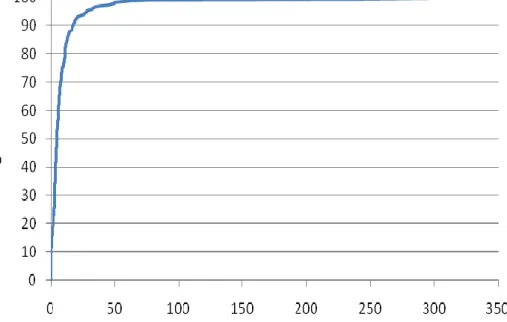
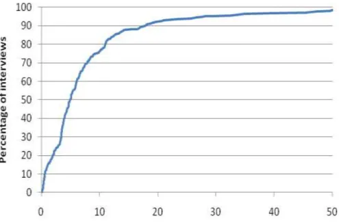
shows the percentage of interviews in relation to the distance travelled. It shows that 90 % of interviews were conducted with visitors who lived less than 17 km away from the location where they were interviewed. Figure 2 shows the same but truncated at 50 km from the interview location. This more clearly shows the relationship at shorter distances, and that 15 % of

interviews were conducted with visitors who lived less than 1 km away from the location where they were interviewed, 50 % within 5 km and 76% within 10km. This suggests that most visitors to Ashdown Forest live close to the site.

Figure 1 Relationship between the linear distance (km) from interviewees’ home postcode and the

(18)

interview location, and the percentage of interviews, truncated at 50 km

3.3 When the same information is separated into those visitors interviewed at the pedestrian access points and those arriving at car parks, as shown in Figure 3, it can be seen that visitors using the pedestrian access points live closer to the site. For example, 67 % of interviews with visitors at the pedestrian access point were with visitors who lived within 2 km, while for those interviewed at the car parks only 6 % lived within 2 km. Increasing the distance to 4 km resulted in 80 % of interviews with visitors at the pedestrian access point and 29 % at the car access point. This suggests that, unsurprisingly, visitors accessing the site at the pedestrian access points tend to live closer to the site than those using the car park access points.

interview location, and the percentage of interviews, separated into pedestrian and car park access points, and truncated at 50 km

(19)

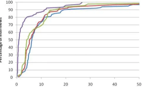
3.4 If the car visitors are further subdivided into those interviewed at previously-defined high, medium and low usage car parks, as in Figure 4, it can be seen that the distance visitors travel to use the car parks is slightly different between car parks of different levels of useage. For example, only 12 % of interviews with car visitors at a high useage car park lived within 4 km, while at medium usage car parks this value was 37 % and 48 % at low usage.This suggests that the high usage access points attract people over a wide range of distances, whereas the low usage access points tend to be used more by local people.

interview location, and the percentage of interviews, separated by high, medium and low usage car parks and pedestrian access, and truncated at 50 km

Visitor Rates in relation to distance

3.5 Visitor rates were calculated in relation to distance for the 20 access points with visitor survey data. To calculate visitor rates, the total number of people observed leaving over the 16 hour period at each interview location was extracted from the tally counts. These tally data describe the total number of visitors recorded at each site over the standard time periods of the survey. For each access point (i) these counts were compared to the number of geo-referenced interviewee postcodes, to give a multiplication factor (Fi) to scale up the interview data. In this way the postcoded visitor data were scaled up to represent total visitor numbers.

Visitor rates (i.e. the mean number of visits per person per year) in relation to distance are shown in

Figure 5,

Figure 6 and

(20)

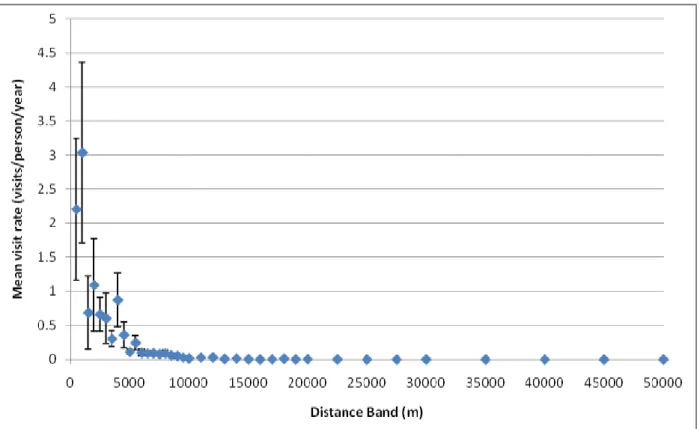
Figure 5 Relationship, with standard error, between the distance from the access point and the mean visit rate, averaged across all access points

Figure 6 Relationship, with standard error, between the distance from the access point and the mean

(21)

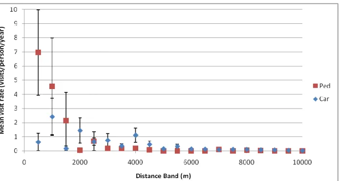
Figure 7 Relationship, with standard error, between the distance from the access point and the mean visit rate, averaged across all access points, separated into foot and car visitors and truncated at 10 km

(22)

4 Modelling and predictions of visit rates

4.1 This section presents the detail of the models used to predict visitor rates at the unsurveyed

access points. We present the full details of the statistical analyses undertaken and technical details of the models used. Later sections then consider the bird data in relation to the visitor data and the implications of the results.

4.2 Actual visitor data are available for the twenty access points surveyed by UE Associates. In order to estimate total visitor numbers to Ashdown Forest and in order to understand the actual distribution of people within the entire site, it is important to estimate how many people may visit the unsurveyed access points. This section therefore explores means by which such estimates can be made.

4.3 We consider people travelling on foot and people travelling by car separately and for these two groups of visitors we use the data from the surveyed access points to derive a means of

predicting visitor rates to the unsurveyed points. The implications of the results are discussed in later sections.

Modelling and predicting foot visitor rate

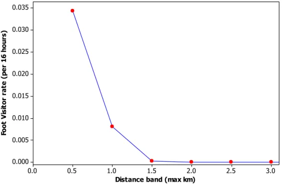
4.4 The rate (Vik) of people visiting any access point (i) of Ashdown Forest (AF) on foot from their home was not related to whether or not there were any parking facilities, but merely declined with distance band (k) from home to the access point (Table 2, Figure 8).

4.5 Based on the UE survey in September 2008, the estimated overall rate of visiting AF on foot via any particular access point within 500m of home was 0.034 per 16 hours of daylight (in

September) (Table 2). Thereafter for every further 500m distance band, foot visitor rates

decreased by about three-quarters and only one interviewed geo-reference visitor who walked to the site lived more than 1500m away (as measured by straight-line distance from home postcode to used access point).

Table 2 Foot visitor rates by bands of distance from home to access point

Distance bandupper limit (km)

Total Residents

Total Observed Visitors per 16hrs allowing for non

geo-referenced visitors

Overall Visitor rate per 16hrs in September 0.5 2048 70.4 0.034361 1.0 7087 57.4 0.008094 1.5 7033 1.6 0.000222 2.0 9605 0.0 0.000000 2.5 16596 0.0 0.000000 3.0 19536 0.0 0.000000

(23)

3.0 2.5 2.0 1.5 1.0 0.5 0.0 0.035 0.030 0.025 0.020 0.015 0.010 0.005 0.000

Distance band (max km)

Fo o t V is it o r ra te ( p e r 1 6 h o u rs )

Figure 8 Foot visitor rates by bands of distance from home to access points

4.6 In order to predict visitor rates for unsurveyed points the foot visitor rates in Table 2 can be used to estimate the number of visitors walking from home to each access point for all of the non-surveyed access points in Ashdown Forest. For each new access point, the number of residents in each 0.5km distance band from the access point is multiplied by the foot visitor rate in Table 2

and then summed across all distance bands to give the predicted total foot visitor number (Vfooti) to access point i.

Modelling and predicting car visitor rate

4.7 In this section we use data on car-park size and the number of residents around access points to try to predict the number of visitors arriving at each point by car.

4.8 The logic of the model fitting approach was as follows: Define:

Gi = Number of geo-referenced visitors to access point i

Gik = Number of geo-referenced visitors to access point i from distance band k Resik = Number of residents in distance band k from access point i

Fi = Multiplier to scale up from geo-referenced visitors to all visitors Then:

observed geo-referenced visitor rate to point i from distance band k = Gik / Resik and

(24)

and

our statistical model to be fitted to our observed visitor data {Gik} is:

Gik = (Resik / Fi) . Pik

which on taking (natural) logarithms to fit a long-linear model becomes: Log(Gik) = Log(Resik / Fi) + Log(Pik)

4.9 We then needed to model the true (or expected) visitor rates (Pik) as a function of factors such as distance and the availability of car parking spaces.

4.10 Previous analyses have shown that the visitor rates for people driving to access points declines with the distance from their home to the access point. The rate of people visiting an access point from a given distance also tends to increase with the number of car parking spaces available at the access point, as shown previously and below.

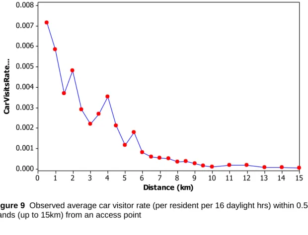
4.11 Figure 9 shows the observed average visitor rate with distance band based on dividing the sum of all car visitors from that distance band to all 20 access points by the sum of all residents at that distance band from each of the 20 access points. The decline in rate with distance is initially steep but then flattens off as several people drive a wide range of relatively large distances to visit Ashdown Forest.

4.12 This is based on access points grouped according to the number of car parking spaces available

(none, 1-25, 26-105, based on 5, 7 and 8 surveyed access points respectively)

4.13 Figure 10 is a similar plot of observed average visitor rate with distance but with separate curves for three groups of access points with differing amounts of car parking spaces: 5 points with none, seven points with 3-25 spaces and 8 points with 26-105 spaces. In this plot, data have been grouped into 2km distance bands because of the relatively low number of residents, and thus visitors, from short distance bands close to the relative small sample of access points in each group. This plot shows that for residents at any distance band, car visitor rate is on average higher to access points where there are more car parking spaces.

(25)

15 14 13 12 11 10 9 8 7 6 5 4 3 2 1 0 0.008 0.007 0.006 0.005 0.004 0.003 0.002 0.001 0.000 Distance (km) C a rV is it sR a te .. .

Figure 9 Observed average car visitor rate (per resident per 16 daylight hrs) within 0.5km distance

bands (up to 15km) from an access point

20 18 16 14 12 10 8 6 4 2 0 0.010 0.008 0.006 0.004 0.002 0.000

Distance band (2km intervals)

C a r v is it o r ra te ( p e r re si d e n t p e r 1 6 d a y lig h t h o u rs ) 0 1-25 26-105 spaces Car parking

This is based on access points grouped according to the number of car parking spaces available (none, 1-25, 26-105, based on 5, 7 and 8 surveyed access points respectively)

(26)

Figure 10 Observed average car visitor rate (per resident per 16 daylight hrs) within 2km distance bands (up to 20km) from an access point

4.14 Therefore, after several stages of trial model development, the following Generalised Log-Linear Poisson model (McCullagh & Nelder, 1989), referred to as Model M1, was found to provide the best fit to the observed geo-referenced car visitor numbers at the 20 surveyed access points: Log(Gik) = Log(Resik / Fi) + a + (b + c Log(Si+1))(Dk)0.75 (Model M1, eqn. 1)

where:

Si = number of car parking spaces at access point i

Dk = upper limit of distance band k in km (0.5km, 1.0km, ..., 50km)

and the term Log(Resik / Fi) is treated as an ‘offset’ variable in the model fitting (McCullagh & Nelder, 1989) so that observed geo-referenced visitors numbers are related to the number of residents (Resik) living within each band and to the fraction (1/Fi) of all observed visitors who were geo-referenced.

4.15 The use of the 0.75 power of distance in the model M1 corrects for the observed slower than exponential pattern of decline in visitor rate with distance.

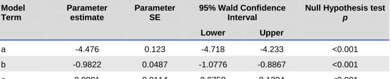
4.16 The standard errors (SE) and significance tests for parameters (a, b and c) in model M1 were estimated by allowing for extra-Poisson variation in the observed visitors (Gik) as represented by the model residual mean deviance of 1.63 (McCullagh & Nelder, 1989), to give the model fitting results in Table 3.

Table 3 Fit Poisson Log-linear Generalised Linear model M1 to the observed geo-referenced vistor

numbers over the 16 hour survey period for 20 access points

Model Term Parameter estimate Parameter SE 95% Wald Confidence Interval

Null Hypothesis test

p

Lower Upper

a -4.476 0.123 -4.718 -4.233 <0.001

b -0.9822 0.0487 -1.0776 -0.8867 <0.001

c 0.0981 0.0114 0.0758 0.1204 <0.001

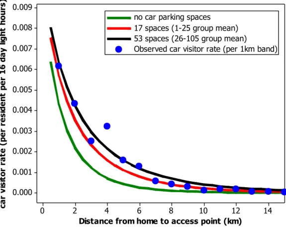
4.17 Illustration lines shows predictions for 0, 17 (mean of group of points with 1-25 spaces) and 53

spaces (mean of group of points with 26-105 spaces. Blue circles denote observed average visitor rates for each 1km distance band.

4.18 Figure 11 gives an illustration of the predictions of car visitor rate with distance relationship based on model M1 for different numbers of parking spaces at access points.

4.19 The predicted number of car visitors (Vcarik) to access point i (with Si car parking spaces) from the Resik people living within distance band k of the access point is therefore given by:

Vcarik = Resik . Pik where Log(Pik) = a + (b + c Log(Si+1))(Dk)0.75 (Model M1, eqn. 2) and the total number of car visitors (Vcari) to access point i is given by:

(27)

14 12 10 8 6 4 2 0 0.009 0.008 0.007 0.006 0.005 0.004 0.003 0.002 0.001 0.000

Distance from home to access point (km)

ca r v is it o r ra te ( p e r re si d e n t p e r 1 6 d a y li g h t h o u rs )

no car parking spaces

17 spaces (1-25 group mean) 53 spaces (26-105 group mean)

Observed car visitor rate (per 1km band)

Illustration lines shows predictions for 0, 17 (mean of group of points with 1-25 spaces) and 53 spaces (mean of group of points with 26-105 spaces. Blue circles denote observed average visitor rates for each 1km distance band.

Figure 11 Predictions of car visitor rate using the fitted model M1 in relation to distance (km) from home

to the access point and the number of car parking spaces available

Predicting total visitor numbers to any access point

4.20 The predicted total visitor per 16 daylight hours (Vtoti) to any access point i is simply the sum of the predicted numbers arriving on foot (Vfooti) and by car (Vcari), namely:

Vtoti = Vfooti + Vcari (eqn. 3)

4.21 This method has been used to derive predictions of the total visitor numbers per 16 daylight hours to each of the 58 non-surveyed access points (and the 20 surveyed points) in the Ashdown Forest SPA area.

4.22 For the 20 surveyed access points, there is a reasonably good relationship between the observed visitor numbers of the 16 hour total surveying period and those predicted from our statistical models based on residents by distance and car space availability (Figure 12). The regression relationship is:

Observed visitors = -24.9 (SE=23.4) + 1.39 (SE=0.27) Predicted visitors

for which the percentage of variation explained (R2) is 60% and the slope of 1.39 is not statistically significant from a slope of 1.0

(28)

250 200 150 100 50 0 250 200 150 100 50 0

Predicted total visits per 16 hours

O b se rv e d t o ta l v is it s p e r 1 6 h o u rs 20 19 18 17 16 15 14 13 12 11 10 9 8 7 6 5 4 3 2 1 1:1

Figure 12 Comparison of observed and model predicted total visitor numbers per 16 daylight hours for

the 20 surveyed access points

Estimates of total visitor numbers (per hour) to Ashdown Forest

4.23 The predictions of visitor numbers for all access points are shown in Map 5, where the visitor numbers to each location are represented by different sized circles, the size of which is proportionate to the number of visitors predicted.

4.24 Across all access points, the total number of visitors predicted to visit the site over the 16 hour period used for the survey is 5198. This reduced to an hourly figure (i.e. divided by 16) is 325 people per hour. These estimates (i.e. for 16 hours and for 1 hour) relate to September, when the survey work was conducted. We do not attempt to extrapolate this further to give an annual figure.

(29)

5 Visual overlays of access

5.1 With a prediction of visitor rates at all access points it is possible to calculate total visitor numbers to the site and to predict how people might distribute themselves across the site as a whole. Visitors were ‘spread out’ from each access point (see methods) to create visual overlays of access levels within the site.

5.2 These visual overlays of visitor numbers are shown in maps 6 – 10. Maps 6 – 8 show, for each 25m cell, the number of visitors within 50m, 100m and 150m respectively. In Map 9 we repeat map 8, with the addition of the Annex I bird species. In Map 10 the same map is shown, without the bird data but showing the distribution of access points and the path network.

(30)

6 Analysis of visitor and bird data to

determine current impacts

6.1 Data from the national surveys for the three Annex I species were used. For the visitable area surveyed these survey results indicated a total of: 77 nightjar (2004 survey), 34 woodlark (2006 survey), and 32 Dartford warbler (2006 survey).

Bird density in relation to nearby visitor and path intensity

6.2 We calculated average bird density in all 25m by 25m cells in each intensity class (1-4) of visitors (VI) or paths (PI) for ‘influence’ distances of 50m, 100, and 150m. The relationships between average bird density and visitor or path intensity are shown for each species in Figure 13. 6.3 Perhaps surprisingly, average bird density was lowest for the cells with the lowest two class

levels of either nearby visitor intensity or path intensity. For woodlark, the highest average density occurs in areas with the highest class levels of visitor intensity at all three assessed influence distances. Average nightjar density was lowest for the quarter of cells with the lowest nearby visitor or path intensity for all three influence distances. Dartford warbler average density was highest amongst the quarter of cells with the highest level of visitor intensity. For each bird species, several of these simple differences in bird density with nearby visitor or path intensity were statistically significant (i.e. test probability p < 0.05; see Table A in Appendix 1).

(31)

Index Intensity PI 50m VI 50m PI 100m VI 100m PI 150m VI 150m 4 3 2 1 4 3 2 1 4 3 2 1 4 3 2 1 4 3 2 1 4 3 2 1 0.025 0.020 0.015 0.010 0.005 0.000 W oo dl ar k de ns it y (p er h a. ) Index Intensity PI 50m VI 50m PI 100m VI 100m PI 150m VI 150m 4 3 2 1 4 3 2 1 4 3 2 1 4 3 2 1 4 3 2 1 4 3 2 1 0.05 0.04 0.03 0.02 0.01 0.00 N ig ht ja r de ns it y (p er h a. ) 0.025 0.020 0.015 0.010 0.005 D ar tf or d w ar bl er d en si ty ( pe r ha .)

(32)

Bird density in relation to habitat type

6.5 Each 25m cell was classified according to its dominant habitat type.

6.6 The numbers and average densities of woodlark, nightjar and Dartford warbler in each of the six main types of habitat within Ashdown Forest SPA are shown in Table 4. There were statistically significant differences between habitats in their average bird density of all three species (based on both Chi-square and likelihood-ratio tests for differences between habitat types in the proportions of 25m cells occupied by a bird species; all test probability p≤0.001).

Table 4 Number and density (per ha.) of woodlark, nightjar and Dartford warbler in each type of habitat

within Ashdown Forest SPA

Habitat Type Area (ha) (%

of total)

Number of birds Bird density (per ha.) (rank)

woodlark nightjar Dartford

warbler woodlark nightjar

Dartford warbler Bracken 747 (29%) 8 30 9 0.011 (5) 0.040 (2) 0.012 (5) Dry Heath 349 (14%) 12 23 13 0.034 (2) 0.066 (1) 0.037 (1) Gorse 63 (2%) 3 2 1 0.048 (1) 0.032 (4) 0.016 (2) Unimproved Grassland 232 (9%) 6 9 3 0.026 (3) 0.039 (3) 0.013 (4) Wet Heath 216 ( 8%) 3 7 3 0.014 (4) 0.032 (4) 0.014 (3) Woodland 979 (38%) 2 6 3 0.002 (6) 0.006 (6) 0.003 (6) Total 2586 (100%) 34 77 32 0.013 0.030 0.012

Chi-square test for habitat differences in the proportion of cells with bird present have null test probability p ≤ 0.001 for all three species.

6.7 The highest densities of woodlark occurred in gorse and dry heath areas, whilst nightjar and Dartford warbler densities were both highest in dry heath, which covered an estimated 14% of the total SPA area. Although woodland was the most widespread habitat (38% of total area), it had much lower average densities for all three species (Table 4). Wet heath also supports lower bird densities than the other habitats.

6.8 It is therefore important to remember and allow for these observed major differences in bird density between habitat types when trying to assess the relationship between local bird

distribution and density and model-predicted nearby visitor pressure. For example, as all three species occur at much lower average densities in woodland, if woodland had lower densities of paths (and thus perhaps visitor pressure) than other habitats, then from an overall analysis

ignoring habitat type, higher bird densities might appear to be the associated with higher path and visitor intensities. More subtly, ignoring habitat type might hide any real relationships between bird distribution and visitor pressure.

Visitor and path intensity in different habitat types

6.9 To assess whether the local intensity of paths and visitor pressure varies with habitat type within Ashdown Forest SPA, we calculated the general level of visitor and path intensity, as measured by the median intensity value (50% higher, 50% lower) separately for the 25m cells in each habitat type. As nearby birds might be only affected by the highest levels of pressure, we also calculated the upper-quartile intensity values (75% less) for each habitat type (Table 5).

(33)

Table 5 Median (50%) and upper-quartile (75%) value of the nearby visitor and path intensity measures for 25m cells in each habitat type

Habitat Number (n) of 25m cells Visitor intensity (VI) within Path intensity (PI) within

150m 100m 50m 150m 100m 50m (a) median (50%) Bracken 11955 647 268 59 29 12 3 Dry Heath 5580 1120 450 97 33 15 4 Gorse 1004 1027 476 135 34 16 5 Unimproved Grass 3713 753 339 97 33 15 5 Wet Heath 3461 356 105 0 17 7 0 Woodland 15669 428 185 37 23 10 3 (b) upper quartile (75%) Bracken 11955 1336 577 150 39 18 5 Dry Heath 5580 2093 893 226 42 19 5 Gorse 1004 2988 1353 359 44 21 6 Unimproved Grass 3713 1593 732 219 42 20 6 Wet Heath 3461 756 292 56 26 11 3 Woodland 15669 870 397 114 33 16 5

6.10 The intensity of paths is lowest in (or very near) wet heath and second lowest in woodland. Even more strikingly, the general level of nearby visitor pressure is much lower in areas of wet heath and woodland than other habitats and much less than half the general visitor levels in area of dry heath which, from Table 4, appear to support the highest levels of bird density.

6.11 This may explain why at the simplest level assessed above, bird density appears highest in areas of high visitor pressure, as recorded above.

6.12 By calculating the ratio of the mean levels of visitor intensity to the mean level of path intensity separately for each habitat type, we estimated the relative intensity of visitor usage of the available paths within (or very near) cells of each habitat type (Table 6). We see that the frequency of usage of paths is on average, lower in wet heath and woodland than the other habitats, especially dry heath, and especially when measured using paths very close by (i.e. within 50m rather than 150m; Table 6).

(34)

Table 6 Relative visitor usage of paths in different habitats as measured by the ratio (VI/PI) of mean visitor intensity to mean path intensity in each habitat type

Habitat Mean visitor intensity (VI)

within

Mean visitor path (PI) within Ratio Mean VI / Mean PI 150m 100m 50m 150m 100m 50m 150m 100m 50m Bracken 1001 432 110 28.4 12.6 3.2 35.2 34.5 110.5 Dry Heath 1503 646 160 32.6 14.3 3.6 46.2 45.3 159.7 Gorse 1859 873 254 34.3 15.7 4.5 54.3 55.6 126.8 Unimproved Grass 1312 615 182 33.3 15.3 4.5 39.4 40.3 90.9 Wet Heath 585 225 50 17.6 6.8 1.5 33.2 33.1 25.1 Woodland 703 327 92 23.1 10.5 2.9 30.5 31.0 30.8

6.13 In the following section we assess the relationship between bird density and visitor or path intensity separately within each habitat type.

Bird density in relation to nearby visitor and path intensity within

habitat type

6.14 To assess visitor and path intensity within habitat types, the relationship between bird density and the nearby intensity of either visitor pressure (VI) or paths (PI) for the cell areas in each individual habitat type are shown in Table B - Table G (Appendix 2) using influence distances of 150m (Table B - Table C), 100m (Table D - Table E) and 50m (Table F - Table G). To aid assessment, average bird densities by habitat and visitor or path intensity class are also shown graphically in Figure A - Figure F (Appendix 2). However, these figures should be used with caution and by referral back to the tables showing the very low numbers of birds on which these average densities are based. If a density is based on one bird location then obviously one recorded bird more or less in the same habitat and intensity level would double the density or reduce it to zero. This is the best available bird information we have to date.

6.15 Being nationally and regionally rare species, the bird numbers are naturally quite low, which can make it difficult to detect statistically significant patterns with both visitor pressure and habitat type. Chi-square tests were used to test whether there were any statistically significant

differences between visitor or path intensity classes within a habitat type in the proportion of cells with a bird species location present.

6.16 The only cases with statistically significant results (i.e. null test probability p <0.05) were in cells classified as bracken and then only when based on the estimate of visitor intensity (VI) or path intensity (PI) within 50m and then only for woodlark with VI (p = 0.036) and PI (p = 0.032) and nightjar with PI (p = 0.003). In these cases, woodlark density did appear to increase with levels of VI and PI, but the pattern of nightjar densities was illogical, being highest for intermediate levels of path intensity within 50m. In retrospect, we think these results for woodlark density increasing with path and visitor intensity in bracken may be an artefact related to the problems of defining and mapping areas of bracken rather than other habitats with scattered bracken.

(35)

7 Discussion: Ecological context and

interpretation of results

Introduction

7.1 Once we allow for the differences between habitat types in average bird densities within Ashdown Forest, we can detect no clear evidence that the current spatial distributions of either woodlark, nightjar or Dartford warbler are affected by the patterns of current levels of nearby visitor pressure or by path intensity within the SPA.

7.2 The analysis has only looked at the distribution of birds within Ashdown Forest, and is difficult as it is focussed on a single site only, rather than being able to compare bird densities or the

distribution of birds across multiple sites with varying levels of disturbance (a more statistically robust approach).

7.3 In this section we discuss the ecological context, drawing comparisons with work on other sites.

Comparison with studies of disturbance at other sites

7.4 This provides a contrast to work on other sites, in particular the work on the Thames Basin Heaths and the Dorset Heaths. For nightjars, several recent studies have demonstrated clear links between human disturbance and both density and breeding success (Liley and Clarke, 2003, Langston et al., 2007b, Clarke et al., 2006, Clarke et al., 2008a, Liley and Clarke, 2002b, Liley and Clarke, 2002a, Langston et al., 2007c, Murison, 2002). Modelling using data from the last national survey (in 2004) for two southern English SPAs suggests that the nightjar population would be 14% higher were there no nearby housing or visitor pressure (Clarke et al., 2008a). Studies have shown a general preference by nightjars for areas away from access points and site edges and a trend for nightjar density to decline with increasing visitor pressure, with nightjars appearing to avoid highly disturbed areas within sites (Liley et al., 2006a, Langston et al., 2007c). A negative correlation has also been shown for urban development or people density and nightjar density, regardless of the size of heathland studied (Liley and Clarke, 2002a, Liley and Clarke, 2002b); urban development density could be considered a rough proxy for recreational access levels.

7.5 Work on breeding success of nightjars has shown that nightjars had significantly higher breeding success at sites with no public access than those with open access. Nests had a greater chance of failure on open access sites with more surrounding urban development and increasing

proximity to a greater density of footpaths (Murison, 2002). Nightjar nests that failed were significantly closer to paths and tended to be closer to the main access points. Incubating

nightjars sit tight unless disturbed; in 2,000 hours of camera observations of eight nests, nightjars never left the nest unattended during the day unless disturbed (Langston et al., 2007a). Flushing during daylight leaves nightjar eggs or chicks vulnerable to predation, the proximate cause of nest failure (Murison, 2002). Use of remote cameras fixed on nests documented a single

instance of predation: The predator was a carrion crow Corvus corone (Woodfield and Langston, 2004b), but this species may be responsible for 60% of nest failures (Murison, 2002).

7.6 Across 16 sites in southern England, woodlark population density was found to be significantly lower at sites with higher disturbance levels (Mallord et al., 2006, Mallord et al., 2007a). This

(36)

reduced the probability of colonisation to below 50%. Mallord’s work resulted in a model to predict the consequences for the woodlark population of a range of visitor access levels (Mallord et al., 2006). Under current access arrangements, a doubling of visitor numbers was predicted to reduce population size by 15%.

7.7 For Dartford warbler, other studies have tried looking at the density of birds across a range of sites with different levels of access and surrounding urban development, and these studies found no clear pattern, with uniformaly high densities of Dartford warblers across all sites (Liley and Clarke, 2002a). Clear impacts on the breeding ecology of Dartford warblers have however been demonstrated, particularly for birds nesting in heather Calluna vulagris dominated (as opposed to gorse Ulex spp dominated) territories (Murison, 2007b, Murison et al., 2007). Disturbance at territories was higher where these were located close to car parks (Murison, 2007b, Murison et al., 2007). Dartford warblers are particularly susceptible to disturbance when nest-building, halting or even abandoning activities when interrupted (Murison, 2007b, Murison et al., 2007). The nearer the centre of the warbler territory is to an access point (e.g. car park), the later the first brood is likely to be raised. Disturbance appears to delay hatching dates and so prevent chick growth from coinciding with periods of optimal invertebrate prey density, and also to interrupt adult foraging and chick feeding (Murison, 2007b, Murison et al., 2007). Dog-walkers accounted for 60–72% of all disturbance events, with dogs off-lead and off-path likely to have the greatest adverse impact on Dartford warbler breeding productivity (Murison, 2007b, Murison et al., 2007). Moreover, for such a short-lived species in which there is also low over-winter survival of young birds, increased disturbance could limit population recovery by reducing annual

breeding productivity and hence the numbers of potential recruits to new areas (Langston et al., 2007a).

7.8 While there is strong and clear evidence of disturbance effects, there does appear to be variation between sites. Emerging work2 from Norfolk, within the Breckland SPA, suggests little impact of disturbance on the breeding success of nightjar or woodlark, through detailed work using nest cameras. In this case there has been no analysis to consider the spatial distribution of the two bird species in relation to access, and also it would appear that visitor numbers and levels of recreational access within the SPA are low in comparison to Dorset and the Thames Basin Heaths, where most of the work on disturbance to the two species has taken place.

Comparison of Ashdown Forest with other sites

7.9 Simple comparison of the density of Annex I bird species at a selection of SPAs in southern England provides a useful wider and contextual reference. In Table 7 we show the number and density of nightjar, woodlark and Dartford warbler on five heathland SPAs in southern England. The comparison is simplistic in that the density estimates do not take into account the habitats present, and each SPA contains areas of unsuitable habitat for the three species such as ancient woodland and mature conifer woodland that cover different proportions of the area of each site. However, the comparison does suggest that Ashdown Forest holds relatively low densities of the three Annex I species, and in particular for Dartford warbler and nightjar (the interest features of Ashdown Forest SPA), densities at Ashdown are lower than on the Dorset Heaths, the Wealden Heaths and on the Thames Basin Heaths (Table 7). The New Forest also appears to hold

particularly low bird densities, an issue that has been raised in other studies (Sharp et al., 2008b). 7.10 The SPAs will all differ in the range and relative areas of habitats present, extent of

fragmentation, types of access, management and climate. Other confounding factors may include the ease of surveying (for example small sites may be easier to survey than large continuous blocks of habitat) and therefore the accuracy of the bird survey data may vary between areas. It is perhaps therefore not surprising that disturbance studies at different sites

2

See: www.breckland.gov.uk/uea_interim_report_to_breckland_19-11-2008.pdf and

Ashdown Forest visitor survey data analysis

Natural England Commissioned Report NECR048