Numerical methods for experimental design of
large-scale linear ill-posed inverse problems
E. Haber, L. Horesh & L. Tenorio
Abstract
While experimental design for well-posed inverse linear problems has been well studied, covering a vast range of well-established design criteria and optimization algorithms, its ill-posed counterpart is a rather new topic. The ill-posed nature of the problem entails the incorporation of regularization techniques. The consequent non-stochastic error introduced by regularization, needs to be taken into account when choosing an experimental design. We discuss different ways to define an optimal design that controls both an average total error of regularized estimates and a measure of the total cost of the design. We also introduce a numerical framework that efficiently implements such designs and natively allows for the solution of large-scale problems. To illustrate the possible applications of the methodology, we consider a borehole tomography example and a two-dimensional function recovery problem.
keywords: experimental design, ill-posed inverse problems, sparsity, constrained optimization.
1
Introduction
During the past decade, data collection and processing techniques have dramatically im-proved. Large amounts of data are now routinely collected and advances in optimization algorithms allow for their inversion by harvesting high computational power. In addition, recent advances in numerical PDEs and in solution of integral equations have enabled us to better simulate complex processes. As a result, we are currently able to tackle high dimensional inverse problems which were never considered before.
However, even when it is possible to gather and process large amounts of data, it is not always clear how such data should be collected. Quite often data are obtained using protocols developed decades ago; protocols that may be neither optimal nor cost-effective. Such suboptimal experiment design may lead to loss of important information and waste of valuable resources.
In some cases, a poor experiment design can be overcome by superior processing tech-niques (the Hubble Space telescope being a typical example), nevertheless, the far best way to achieve an ‘optimal’ design is by proper design of the experimental setup. The field of
experimental design has a long history. Its mathematical and statistical foundations were pioneered by R. A. Fisher in the early 1900s. It is now routinely applied in the physical, bi-ological and social sciences. However, almost all the work in the field has been developed for the over-determined, well-posed case (e.g., [4, 5, 17, 1] and references therein). The ill-posed case has remained under-researched. In fact, this case is sometimes completely dismissed. For example, in [17] we read: ‘Clearly, for any reasonable inference, the number n of obser-vations must be at least equal tok+ 1’ (kbeing the number of unknowns). Conversely, many practical problems, and in fact, most of the geophysical and medical inverse problems, either characterized by possessing a smaller of observations than unknowns or are ill-posed in the usual sense. Experimental design for such problems has remained largely unexplored. For ill-posed problem, we are only aware of the work of [7, 13], who used techniques borrowed from the well-posed formulation, and the work of [18]. But none of these papers details a coherent and systematic approach for experimental design of ill-posed problems. We are only aware of two papers that address this problem in a more systematic way. Our approach shares some similarities with the very recent work of Bardow [3], but we consider a more general approach to control the mean square error of regularized Tikhonov estimators for large-scale problems. Another very recent work was published by Stark [21].His approach, was based on generalizations of Backus-Gilbert resolution. In this formulation control over the mean squared error is also considered. Our approach focuses on the use of training models and on actual numerical implementations, especially for large-scale problems.
Many important inverse problems are large in practice, the number of parameters that need to be estimated can range from tens of thousands to millions. The computational techniques for optimal design proposed so far in the literature were not suitable for such large-scale problems. Most of the studies that have investigated the ill-posed case, as mentioned above, employed computational techniques that were based on stochastic optimization. Such an approach is prohibitively computationally expensive.
In this paper, we develop an optimal experiment design (OED) methodology for ill-posed problems. This methodology can be applied to many practical inverse problems and, although only the linear case is considered here, it can be generalized to nonlinear problems. We develop mathematical tools and efficient algorithms to solve the optimization problems that arise in the experimental design. In fact, the problem is formulated in a way that allows the application of standard constrained optimization methods.
The rest of the paper is organized as follows: The basic background on experimental design for well- and ill-posed linear inverse problems is reviewed in Section 2. In Section 3 we propose several experimental designs for ill-posed problems and discuss issues related to the convexity of the objective functions which define these designs. In Section 4 we present numerical optimization algorithms for the solution of the optimization problems that arise from this formulation.In Section 5 we present two numerical examples: a borehole tomographic inversion and a two-dimensional function recovery problem. Finally, in Section 6 we summarize the paper and discuss future research.
2
From classical to ill-posed OED
We begin by reviewing the basic framework of OED in the context of well-posed inverse problems of the following type: The data are modeled as
d=K(y)m+ε, (2.1)
where K(y) is an `×k matrix representation of the forward operator that acts upon the model m and depends on a vector of experimental parameters y ∈ Y. The noise vector ε
is assumed to be zero mean with iid entries of known variance σ2. The experiment design question is constructed into the selection ofythat leads to an optimal estimate ofm. Solution of this problem for a continuous vectorycan be very difficult. For example, in many practical problems the matrixK(y) is not continuously differentiable iny, in other cases where it does, its derivative may be expensive or hard to compute.This implies that typical optimization methods may not be applicable. We therefore reformulate the OED problem by discretizing the space Y. This approach has also been used for the well-posed case (e.g., [17]).
Assume thatyis discretized asy1, ..., yn, which leads ton possible experiments to choose
from:
di =Ki>m+εi (i= 1, . . . , n), (2.2)
where for simplicity eachKi>is assumed to be a row vector representing a single experimental setup. In the general case, each K(yi)> may be a matrix. The goal is to choose a number
p < n of experiments that provides an optimal estimate (in a sense yet to be defined) of m. (Of course, the well-posed case considered first requires p > k.)
We begin by reviewing the approach presented in [17]. Let qi be the number of times
Ki is chosen (hence 1>q = p). Finding the least squares (LS) estimate of m based on qi
independent observations of Ki>m (i = 1, ..., n) is equivalent to solving for the weighted LS estimate: b m= arg min n X i=1 qi di−Ki>m 2 = arg min (d−Km)>Q(d−Km),
where Var(di) = σ2/qi (for qi 6= 0), Q = diag{q1, ..., qn} and K is the n×k matrix with
rows Ki> (the reduction in the variance of di comes from averaging the observations which
correspond to the same experimental unit). Assuming that K>QK is nonsingular, we can write
b
m= K>QK−1K>Q d, (2.3) which is an unbiased estimator of m with covariance matrix σ2C(q)−1, where
C(q) =K>QK. (2.4) Since mb is unbiased, it is common to assess its performance using different characteristics of its covariance matrix. For example, the following optimization problem can be used to
choose q:
min
q trace C(q)
−1 (2.5)
s.t. qi ∈N∪ {0}, 1>q =p.
This is known as an A-optimal experiment design. If instead of the trace, the determinant or theL2 norm ofC(q)−1 is used, then the design is known asD- orE-optimal, respectively.
Since the OED (2.5) is a difficult combinatorial problem, we may use instead an approx-imation based on the relative frequencywi =qi/n that each Ki is chosen. The weighted LS
estimate and its covariance matrix are given by (2.3) and (2.4) with w in place of q. The optimization problem (2.5) then becomes:
min
w trace C(w)
−1
(2.6) s.t. w≥0, 1>w= 1.
Given a solutionwof (2.6), the integer part ofn w provides an approximate solution of (2.5) which improves as n increases.
A discussion of A-, D- and E- designs can be found in [4, 17]. As noted above, these designs are defined by weighted LS solutions based on averages of the repeated observations of different experiments. We shall refer them as cost-controlled designs to distinguish them from the designs defined in the next section. For cost-controlled designs, the total cost (the sum of all the weights of the experiments) is controlled by the constraint 1>w= 1, the new designs control the total cost in a different way.
2.1
Sparsity-controlled designs
We now propose a new formulation that in some applications may be more appropriate than the cost-controlled designs; we refer to this formulation as sparsity control design (SCD). In the applications we have in mind, the number of possible experimental units is very large but only a few are needed or can be realistically implemented. This implies that w should have only a few nonzero entries (i.e., w is sparse). The formulation and solution of this problem can be obtained by including a regularization term in (2.6) that penalizes w using a norm that has some control over the sparsity of w.
In order to obtain a sparse solutionw, one would naturally use anL0 penalty (recall that
the ‘zero-norm’kwk0 is defined as the number of nonzero entries ofw). However, this type of
regularization leads to a difficult combinatorial problem. Instead, we use L1 regularization,
which still promotes sparse solutions (e.g., sparser than an L2 penalty).
The merits for employing an L1 penalty with an L2 misfit can be found in [8], this
study also includes a comprehensive analysis of the expected sparsity properties of solutions acquired by this framework. However, the objective function of our problem is not an L2
misfit inw. In Section 4, we considerL1 regularization and a heuristic approximation of the
L0 approach for our OED problem. We show that the L0 heuristic may outperform the L1
In summary, an A-optimal sparsity-controlled design is defined as a solution of the fol-lowing optimization problem:
min
w trace C(w)
−1 +βkwk
p (2.7)
s.t. w≥0,
where 0 ≤ p ≤1 and β > 0 is selected so as to obtain a desired number of nonzero wi. In
this paper we will only considerp= 1 and an approximation to the p= 0 problem.
To a practitioner, a solution wof (2.7) means that all the observations that corresponds to a nonzerowishould be carried out so as to provide a varianceσ2/wi. This can be achieved,
for an instance,by adjusting the measuring instrument or extending the observation time. The estimate of mis then obtained using weighted LS. In some cases, the experimenter may have a maximum allowable variance level. In such case, a constraintw≤wmaxcan be added
to (2.7).
Although problems (2.7) and (2.6) may seem different, it is easy to verify that a solution of (2.7) with p = 1 and an appropriate choice of β is also a solution of (2.6). It is also important to note that p = 0 may lead to a design that that achieves a smaller value of trace C(w) for the same number of nonzero entries in w. We explore this issue further in the numerical examples.
2.2
The Ill-posed case
Since the designs discussed so far have been based only on the covariance matrix, they are not appropriate for ill-posed problems where estimators ofm are most likely biased. In fact, the bias may be the dominant component of the error. We now draw our focus towards the ill-posed case.
LetW = diag{w1, ..., wn}be again a diagonal matrix of non-negative weights and assume
that the matrixK>W Kis ill-conditioned. A regularized estimate ofmcan be obtained using penalized weighted LS (Tikhonov regularization) with a smoothing penalty matrix L:
b
m = arg min (d−Km)>W(d−Km) +αkLmk2,
where α >0 is a fixed regularization parameter that controls the balance between the data misfit and the smoothness penalty. Assuming that K>W K +α L>L is nonsingular, the estimator is mb = K>W K+α L>L−1K>W d,whose bias can be written as
Bias(mb ) =Emb −m=−α K>W K+α L>L−1L>L m.
Since the bias is independent of the noise level, it cannot be reduced by repeated observations. The effect of the noise level is manifested in the variability ofmb around its mean Emb. Thus, this variability and the bias ought to be taken into account when choosing an estimator.
Define B(w, m) = kBias(mb)k2 and V(w) = Ek
b
m−Emb k2/σ2. The sum of these two
the mean squared error (MSE) ofmb. More precisely, the MSE ofmb is defined asEkmb−mk2,
which can also be written as:
MSE(mb ) = Ekmb −Emb +Emb −mk2 =kE b m−mk2+Ek b m−Emb k2 = kBias(mb)k2+Ek b m−Emb k2 =α2B(w, m) +σ2V(w).
The following lemma summarizes some of the characteristics of the Tikhonov estimate for a general symmetric matrix W and correlated noise with covariance matrix σ2Σ. The
proof follows from simple repeated applications of the formula for the expected value of a quadratic form: If x is a random vector of mean µ and covariance matrix σ2Σ, then Ex>Q x=µ>Q µ+σ2trace(QΣ ). More details can be found in [15, 22].
Lemma 1 Letd=Km+ε, whereK is ann×kmatrix and εis a zero mean random vector with covariance matrixσ2Σ. Letα >0 be a fixed regularization parameter,W a symmetric
matrix and L anr×k matrix such that K>W K+α L>Lis nonsingular. Define
b
m = arg min (d−Km)>W(d−Km) +αkLmk2, (2.8) and the matrix
C(w) =K>W K+α L>L. (2.9) Then:
(i) The Tikhonov estimate of m is:
b
m =C(w)−1K>W d. (2.10) (ii) Its mean squared error is:
MSE(mb) = Ekmb −mk2 =α2B(W, m) +σ2V(W), (2.11)
where
B(W, m) = kC(w)−1L>Lmk2, V(W) = trace
W K C(w)−2K>WΣ
. (2.12)
The idea is to define optimization problems similar to (2.7) but with an objective function that measures the performance of mb taking into account its bias and stochastic variability. A natural choice would be the MSE , however, this measure depends on the unknownm. In the next section we consider different ways to control an approximation for the MSE that are based on different assumptions on m.
3
Design criteria for Ill-posed problems
As we have seen in Section 2, to obtain an optimal design based on Tikhonov regularization estimators, the deterministic and stochastic components of the error have to be taken into account. This is done by controlling the overall MSE. We modify the designs presented in Section 2 to use MSE(mb ) =α2B(w, m) +σ2V(w) as the main component of the objective
function.
The problem is that the bias component B(w, m) depends on the unknown model m. There are different ways to control this term ; these depend on the available information and on how conservative we are willing to be. For example, if we know a-priori thatkL>Lmk ≤
M, then Lemma 1 with W = diag{w1, ..., wn} leads to the bound
B(w, m) = kC(w)−1L>Lmk2 ≤ kC(w)−1 k2M2.
But this bound may be too conservative. We will instead consider average measures of B(w, m) that are expected to be less conservative.
(a) Average optimal design
Assuming that the model is in a bounded convex setM, we consider the average of B(w, m) over Mand define the approximation
AOD : MSE(\ w) = α 2 R Mdm Z M B(w, m)dm+σ2V(w). (3.13) The downside of this design is that it does not give preference to ‘more reasonable’ models inM. Unless the set Mis well constrained, such design may be overly pessimistic.
(b) Bayesian optimal design
In order to assign more weight to more likely models,m is modeled as a random vector with a joint distribution function π. The average ofB(w, m) is now weighted byπ:
BOD : MSE(\ w) = EπMSE(mb) = α
2
EπB(w, m) +σ2V(w). (3.14)
For example, if m is Gaussian N(0,Σm), then (3.14) reduces to
\
MSE(w) = α2traceB(w) ΣmB(w)>
+σ2V(w), (3.15) with B(w) = C(w)−1L>L.
Note that the distributionπ is not required for computation ofEπB(y, m) in (3.14); only
the covariance matrix ofm is needed. Hence, whenever data are available for estimating the covariance matrix, the design can be approximated.This rationale leads us to the empirical design.
(c) Empirical Bayesian design
In many practical applications, it is possible to obtain examples of plausible models. For example, often in geophysical applications the Marmusi model [23] is used to test inversion algorithms. In medical imaging the Shepp-Logan model is frequently used as a gold standard to test different designs and inversion algorithms [20]. There are also geostatistical methods to generate realizations of a given media from a single image (e.g., [19] and references therein). Finally, for some problems there are databases of historical data that can be used as reference. Letm1, ..., ms be examples of plausible models which will be henceforth referred as
train-ing models. As in the Bayesian optimal design, it is assumed that these models are iid samples from an unknown multivariate distributionπ, only that this time we use the sample average b EπB(w, m) = 1 s s X i=1 B(w, mi), (3.16)
which is an unbiased estimator of EπB(y, m). We thus define the following approximation:
EBD : MSE(\ w) =α2EbπB(w, m) +σ2V(w). (3.17)
This type of empirical approach is commonly used in machine learning where estimators are trained using iid samples. We have previously used a similar approach to choose regulariza-tion operators for ill-posed inverse problems [10].
The computation of (3.16) can be further simplified when the covariance matrix of m
is modeled as a function of only a small set of parameters that can be estimated from the training models. Here, we focus on the more difficult case when no such covariance model is used.
Clearly, Bayes’ theorem has not been used in the definition of the ‘Bayesian’ designs. To justify the name, consider the cost-controlled design and assume that m is Gaussian
N(0,Σm) with Σm = σ
2
α(L
>L)−1 (Lcan be defined so thatL>L is nonsingular) and that the
conditional distribution of d given m is also Gaussian N(Km, σ2Σ) with Σ = (W +δI)−1.
Then, as δ →0+, (3.15) converges to \
MSE(w) =σ2trace K>W K +α L>L C(w)−2=σ2traceC(w)−1, (3.18) where C(w) is defined in Lemma 1. It is easy to see that (3.18) is precisely the trace of the covariance matrix of the posterior distribution of m given d. Hence, the term ‘Bayesian’ in the name of the design. It is, in fact, anA-optimal Bayesian design [5]. (Note that the AOD is a BOD with a flat prior and an EOD is a BOD with the empirical prior)
These three designs lead to an optimization problem that generalizes (2.7) to the ill-posed case:
min
w Jb(w) = \MSE(w) +βkwkp (3.19)
Three important remarks are in order:
(1) OED and tuning of regularization parameters. The search for appropriate weights wi can be interpreted as the usual problem of estimating regularization parameters
for an ill-posed inverse problem. The method we propose determines w that minimizes the MSE averaged over noise and model realizations. This is done prior to collecting data. Although it is possible (and in many cases desirable) to obtain a regularization parameter adapted to a particular realization of noise and model m, experimental design is conducted prior to having any data. It is therefore sensible to consider values of the regularization parameters that work well in an average sense.
(2) Selecting α. It is clear that the Tikhonov estimate of m and its MSE depend on α only through the ratio w/α but α itself is not identifiable. It is only used to calibrate (by preliminary test runs)w to be of the order of unity. This facilitates the identification of
wi that are not significantly different from zero.
(3) Convexity of the objective function. The formula for the error term V(w) is different in the well- and ill-posed cases. In the former, the variance of an individual experiment is controlled by averaging observations of the same experimental unit. In the ill-posed case, the variances of averaged observations are not used as weights. This time the wi are just weights chosen so that the weighted Tikhonov estimator of m has a
good MSE. One reason for this change is convexity. In the well-posed case, the function
w → traceC(w) is convex (see also [4]), so the optimization problem can be easily solved by standard methods. This is no longer true with ill-posed problems ; for in this case we have V(w) = trace W K C(w)−2K>; a function that can have multiple minima. Instead, the new approach yields V(w) = trace W K C(w)−2K>W
, which is better behaved. For example, in the simple case when K =L = I and α = 1, we have V(w) = P
wi/(1 +wi)2
for the well-posed case. This function is obviously not convex and has multiple minima. On the other hand, the ill-posed formula reduces to V(w) =P
w2
i/(1 +wi)2. This function is
again not convex but it is quasi-convex (i.e., it has a single minimum).
On the other hand, it turns out that the estimate of B(w, m) defined for each of the three designs is a convex function of w:
Lemma 2 Let m have a prior distribution π with finite second moments. Then EπB(w, m)
is a convex function of w.
Proof: Let µ and Σm =R>R be, respectively, the mean and covariance matrix of m under
π. Then EπB(w, m) = kC(w)−1L>L µk2+ trace R L>L C(w)−2L>L R> (3.20) = kC(w)−1L>L µk2+X k kC(w)−1L>L R>ekk2,
where ek is the canonical basis of Rn. Hence, it is enough to show that for any b ∈Rn, the
functionB(w) =b>C(w)−2bis convex, where C(w) = K>diag(w)K+α L>L. We do this by
showing that B(w) is convex along any line in the domain ofw: Letwbe a vector with non-negative entries and z a direction vector. Define the scalar functionf(t) = b>C(w+tz)−2b.
We show that f(t) is convex for all t such thatw+tz ≥0. Define x implicitly by
C(w+tz)x=K>diag(w+tz)K+αL>L x=b, (3.21) so that f(t) = x(t)>x(t). Differentiation of f leads to
˙
f = 2x>x˙ and f¨= 2 ˙x>x˙ + 2x>x,¨ while differentiation of (3.21) with respect to t yields
K>ZKx+C(w+tz) ˙x= 0 and 2K>ZKx˙+C(w+tz) ¨x= 0, (3.22) where Z = diag (z). Since ¨f = 2kx˙k2 + 2x>x¨, showing that x>x¨ ≥ 0 is enough to prove
the non-negativity of ¨f. Using (3.22), we obtain
x>x¨ = −2x>C(w+tz)−1K>ZKx˙ = 2x>C(w+tz)−1BC(w+tz)−1Bx= 2x>G2x,
where B = K>ZK and G = C(w +tz)−1B. Since C(w+ tz) is symmetric and pos-itive definite, there is a nonsingular matrix S such that C(w +tz) = S>S. Note that (S>)−1 S>SB
S>=SBS>.This means thatGandSBS>are similar matrices and there-fore, since B is symmetric, G is diagonalizable: There is a nonsingular matrix T such that
G=TΛT−1, where Λ is a diagonal matrix of eigenvalues ofG. It follows that G2 =TΛ2T−1
and therefore x>G2x≥0. Hence ¨f ≥0 and b>C(w)−2b is a convex function.
Despite the convexity of the bias term, the estimate of the MSE is non-convex because of the non-convexity of V(b w). There are two reasons why the non-convexity of the objective
function may not be critical. First, while it is desirable to find an optimal design, any improvement on a currently available one may be sufficient in practice. Second, in many ill-posed inverse problems the stochastic errorV(w) is small compared to the bias component B(w, m).
4
Solving the optimization problem
The framework presented in Section 3 is a new approach that can be applied to a broad range of linear and linearized optimal experimental designs of ill-posed inverse problems. Before discussing a solution strategy, we need to define numerical approximations for the estimates of the MSE.
Since the weights wi are non-negative, the non-differentiableL1-norm can be replaced by
1>w; which leads to a large but tractable problem. However, the computation of a quadratic form or a trace involves large, dense matrix products and inverses which cannot be acquired
efficiently in large-scale problems. Hence, we now derive approximations of the objective function that do not require the direct computation of traces or matrix inverses.
In order to estimateV(w), we need to approximate the trace of a possibly very large ma-trix. Stochastic trace estimators have been successfully used for this purpose. In particular, Golub and von Matt [9] have used a trace estimation method proposed by Hutchinson [11]. in which the trace of a symmetric positive definite matrixH is approximated by
trace(H)≈ 1 s s X i=1 vi>Hvi, (4.23)
where eachviis a random vector of iid entries taking the values±1 with probability 1/2. The
performance of this estimator was numerically studied in [2] with the surprising result that the best compromise between accuracy and computational cost is achieved withs = 1. Our numerical experiments confirm this result. We therefore use the following approximation:
b
V(w) =v>W KC(w)−2K>W v=w>V(w)>V(w)w, (4.24) where V(w) =C(w)−1K>diag (v).
If the mean and covariance matrix of m are known, then the expected value of B(w, m) is given by (3.20); this still requires the computation of a norm and a trace. Nevertheless, we consider the more general case where the mean and covariance matrix ofmare estimated based on iid samples m1, ..., ms. We use the sample estimate defined for the EBD:
b B(w) = 1 s s X j=1 m>j B(w)>B(w)mj, B(w) =C(w)−1L>L. (4.25)
Summarizing, the approximation to the optimization problem (3.19) that we solve for the casep= 1 is:
min w Jb(w) =α 2 b B(w) +σ2Vb(w) +β e>w (4.26) s.t. w≥0.
4.1
Numerical solution of the optimization problem
For solution of (4.26), we use projected gradient and projected Gauss-Newton methods. This requires the computation of the gradients of Bband V. We have:b
∇w w>V(w)>V(w)w= 2Jv(w)>V(w)w ∇w m>B(w)>B(w)m= 2Jb(w)>B(w)m, where Jv(w) = ∂[V(w)w] ∂w and Jb(w) = ∂[B(w)m] ∂w .
We use implicit differentiation to obtain an expression for the matrices Jv and Jb. Define
rb = K>W K +αL>L
−1
K>W K m.
The matrix Jb is nothing but ∇wrb. Differentiating rb with respect to to w leads to
K>diag (Km) = K>W K +αL>L ∂rb ∂w +K > diag (Krb), which yields Jb =C(w)−1K>diag [K(m−rb) ]. (4.27)
We proceed in a similar way to obtain an expression forJv. First, note that
∂[V(w)w]
∂w =V(w) +
∂[V(w)wfixed]
∂w .
To compute the second term in the above sum, write
rv =V(w)wfixed = K>W K +αL>L
−1
K>diag (v)wfixed.
Differentiating this equation with respect to w leads to
K>W K +αL>L ∂rv
∂w +K
>
diag (Krv) = 0,
which finally yields
Jv =V −C(w)−1K>diag (Krv). (4.28)
This completes the evaluation of the derivatives of the objective function. It is important to note that neither the matrix C(w) nor its inverse are needed explicitly for computation of the objective function or any of the gradients. Whenever a product of the form C(w)−1u is
needed, we simply solve the system C(w)x = u. To solve such system, only matrix-vector products of the formC(w)v are required.
Having found the gradient, we can now use any gradient-based method to solve the problem. We have experimented with the projected gradient formulation, which requires only gradient evaluation, as well as the projected Newton method. For the Gauss-Newton method, one can approximate the Hessian of the objective function Jb in (4.26)
by
∇2J ≈b σ2Jv>Jv +α2Jb>Jb.
With the Jacobian at hand, it is possible to use the method suggested by Lin and Mor´e [12]. The active set is (approximately) identified by the gradient projection method and a truncated Gauss-Newton iteration is performed on the rest of the variables. Again, it is important to note that the matrices Jv and Jb need not be calculated. A product of either
with a vector involves a solution of the system C(w)x=u. Thus, it is possible to facilitate conjugate gradient for computation of an approximation of a Gauss-Newton step.
Beyond the obvious computational benefits offered by a design framework that relies merely on matrix-vector products, an even more fundamental advantage applies.Many imag-ing systems, such as tomographs, employ hardware-specific computational modules, or in other cases, a black box code module is in use. These modules are often accessible only via matrix-vector products. Thus, the proposed methodology can be easily applied for these cases, using the current customized computational machinery.
4.2
Approximating the
L
0solution
Although it is straightforward to solve the L1 regularization problem, one can attempt to
approximate the L0 solution. The L0 solution is the vector w with the least number of
nonzero entries. Obtaining this solution is an intricate combinatorial problem. Nevertheless, it is possible to approximate theL0 solution using the L1 penalty.
Write{1, ..., n}=I0∪IA, whereI0 contains all the indices for the zero entries ofwandIA
contains the rest. We write wI0 and wIA for the restrictions of w to I0 and IA, respectively.
If I0 were known a priori, the L0 solution could be obtained by defining wI0 = 0 and by
solving the unregularized optimization problem min wIA J(wIA) = α2 s s X j=1 m>j B(wIA) > B(wIA)mj +σ 2w> IAV(wIA) > V(wIA)wIA (4.29) s.t wIA ≥0 wI0 = 0.
This problem does not require any regularization term because the zero set is assumed known. The combinatorial nature of the L0 problem emerges due to the search for the
set IA. Nevertheless, one can approximate IA with the corresponding index set of the L1
solution.
This idea has been explored in [4], where numerical experiments show that the approx-imate L0 solution may differ, and in fact, improve on the L1 solution. In this work we use
the same approximation: We set the final weights to those that solve (4.29) with the set IA
obtained from the solution of the L1 problem.
5
Numerical examples
We present two numerical examples that illustrate some applications of the proposed method-ology. These examples show that experimental design is potentially of great significance for practical applications.
5.1
A borehole tomography problem
We begin with a ray tomography example that is often used for illustrative purposes in geophysical inverse problems. It also serves as a point of comparison as it has been used in [7, 18] for their experimental design work.
The objective of borehole ray tomography is to determine the slowness (inverse of veloc-ity) of a medium. Sources and receivers are placed along boreholes and/or on the surface of the earth and travel times from sources to receivers are recorded. The data (travel times) are modeled as
dj =
Z
Γj
m(x)d`+εj (j = 1, . . . , n), (5.30)
where Γj is the ray path traversing between source and receiver. In the linearized case
considered here, the ray path does not change as a function of m (see for example [16]). In this case, the goal of experimental design in this case is to choose the optimal placement of sources and receivers.
Figure 1 shows a sketch of the experimental setup used in our numerical simulation. The medium is represented by the square region [0,1]×[0,1] with boreholes covering the interval [0,1] on each of the sides. The top represents the surface, which also comprises the interval [0,1]. The model is discretized using 64×64 cells.
Figure 1: Geometry of the borehole tomography example. Sources and receivers are placed along the two boreholes (left and right sides of the square region) and on the earth’s surface (top). The lines represent straight ray paths connecting sources and receivers.
Sources and receivers are to be placed anywhere in the design space Y = I1 ∪I2 ∪I3,
where I1 ={(x, y) : x= 0, y ∈[0,1]}, I2 ={(x, y) : x= 1, y ∈[0,1]} and I3 ={(x, y) :
y= 0, x∈[0,1]}. We are free to choose rays that connect any point on Ik to a point on Ij
(j, k = 1,2,3; j 6=k). We discretize eachIi using 32 equally-spaced points. This gives a total
of 322×3 = 3072 possible experiments. Our goal is to choose the optimal placement of 500
sources and receivers. For the solution of the inverse problem we have used the discretization of the gradient as a smoothing matrix.
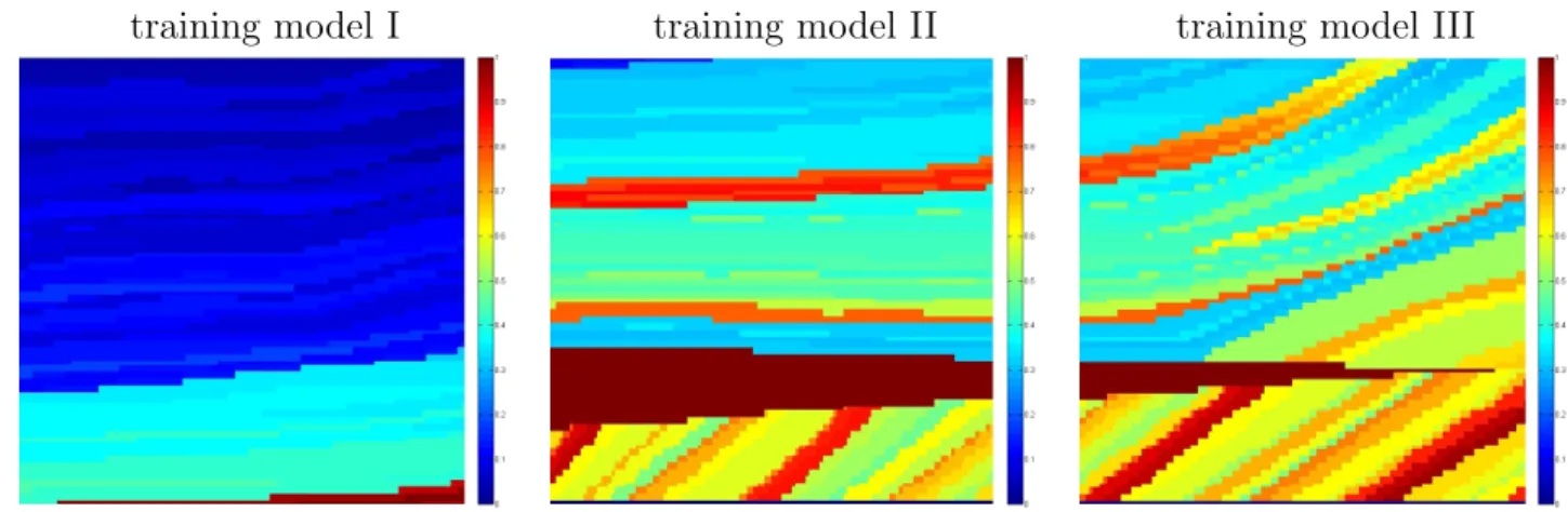
To create the set of training models, we divide the Marmousi model [23] into four
testing its performance. The training models are shown in Figure 2 and the testing model in Figure 3.
training model I training model II training model III
Figure 2: The first three training models obtained from the Marmusi model.
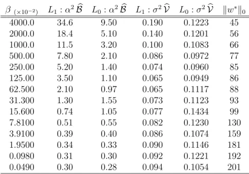
The code that minimizes Jb was executed with different values of β. Table 1 shows the
final values of B(b w∗), V(b w∗) and the sparsity of the solution w∗ for some different values of
β. The results are shown for the L1 penalty and the L0 approximation.
Note that the minimum of the objective function comprises a bias term Bbwhich is
sub-stantially larger than Vb. This ascertains that methods for optimal experimental design of
ill-posed problems must take the bias into consideration as it may play a more important role than the variance. This can be interpreted as a problem with the chosen regularization operator. In fact, we have used a similar strategy in order to choose appropriate regular-ization operators L for ill-posed problems [10]. Of course, the importance of the bias is noise-dependant. For this example, we would need the noise level to be thirty times larger so that the variance component will be of the same order as the bias term. Note also that in many cases there is a difference between the results from the L0 and L1 designs. Typically,
the L0 design gave a smaller MSE estimate than the L1 design.
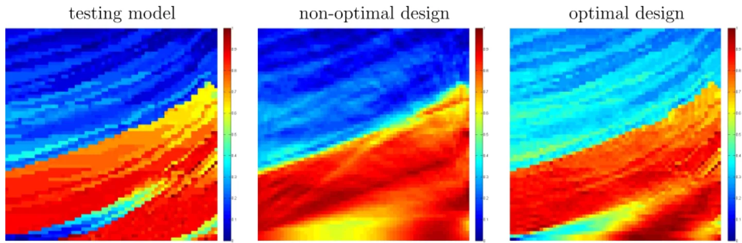
In order to assess the performance of the optimal design obtained by the code, we simulate data using the test model m4 and use the optimal weights for its recovery. We compare this
estimate with the one obtained using the weights based on a uniform placement of sources and receivers. For the sake of objectivity, equal number of active sources in and receivers were deployed for both designs. This number was determined according to the optimum obtained for β = 10−2 Y. The error kmˆ(w)−mk was 1.7×10³ for the optimal design and
3.1×10³ for the other. Figure 3 shows the estimates ofm
4 obtained with the two designs. It
is evident that optimally designed survey yielded a substantial improvement in the recovered model.
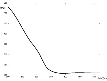
Another important feature of our design is its controlled sparsity. The number of nonzero entries in wis reduced by decreasing β. It is then natural to ask for a method to choose an ‘optimal’ number of experiments. To answer this question, the MSE is plotted as a function of the number of non-zeros in the design. The plot is shown in Figure 4. The graph shows a
β (×10−2) L1 :α2Bb(×102) L0 :α2Bb(×102) L1 :σ2Vb (×10−1) L0 :σ2Vb (×10−1) kw∗k0 1000.0 4.3 3.1 0.51 0.98 249 130.00 2.4 2.1 2.70 1.50 310 16.000 2.1 2.1 2.80 1.70 423 2.0000 2.1 2.1 2.90 1.38 491 0.2400 2.1 2.1 2.90 3.40 507 0.0310 2.1 2.1 2.90 3.60 519
Table 1: Sparsity of the optimal w∗ and components of the MSE estimate at w∗ for the tomography simulation. The results are shown for different values of β and for the L1 and
L0 designs.
testing model non-optimal design optimal design
Figure 3: The test modelm4 (left) and its estimates obtained with the non-optimal (middle)
and optimal (right) designs.
clear L-shape with the MSE decreasing significantly in the region kwk0 ≤350 and without
significant improvement beyond this point. This suggests that selection of the number of experiments at the corner point 350 where the MSE stabilizes, may provide a cost-effective compromise. This example also shows that there is a point of diminishing return. Resources may be invested to obtain more data but the improvement in the MSE may not be significant.
5.2
Recovery of a function from noisy data
For a second example, we consider noisy observations of a sufficiently smooth function
f(x1, x2) on Ω = [0,1]×[0,1] (e.g., f ∈C2(Ω)):
di =f(xi1, x
i
2) +εi (i= 1, . . . , n). (5.31)
The goal is to recover the values of the function on a dense gridG ⊂Ω from values observed on a smaller, sparse grid S ⊂ G. The design question is to determine S. This is a common
Figure 4: MSE as a function of sparsity (kwk0 = NNZ(w)) of the optimal w obtained with
the L0 heuristic on the tomography simulation.
practical problem that arises, for example, in air pollution monitoring where one wishes to set the placement of the sensors (e.g., [6] and reference therein). In this type of applications pollution map database from previous years is available, and can be used as a source of training models. As in the tomography problem, we begin by discretizing Ω. We use a uniform grid G of `×` nodes and assume that sensors can be placed in any of its nodes. We write fh for the vector of values off on G. Let W = diag (w) be the matrix of weights
assigned to each node. The Tikhonov estimate of fh that uses the discrete Laplacian ∆h as
smoothing penalty is defined as the minimizer of (fh−d)
>
W(fh−d) +αk∆hfhk2, where
∆h is a discretization of the Laplacian (e.g., [24, 14]). The subset S of the grid is defined by
the nonzero entries in w.
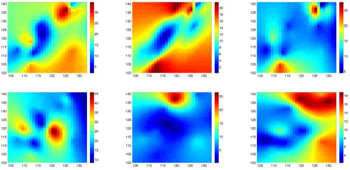
We run our algorithm using a training set of 1000 maps randomly chosen from the available 5114 maps of daily air pollution data (NO2) for the years 2000-2007 in the
Ashkelon/Ashdod region (Israel). Six of the maps are shown in Figure 5. The goal is to determine the optimal location of air-pollution stations in the same region. In order to use our method we need the varianceσ2 of the data. The value 0.1 of this variance was provided by the atmospheric scientists; it was obtained from the known performance characteristics of the instruments.
The results are summarized in Table 2. Once again the table shows that the bias term is more significant than variance term V. Thus an experimental design based only on the covariance matrix would yield poor results. Also, just as in the tomography example, the
Figure 5: Maps of air pollution in the Ashkelon/Ashdod area.
L0 design gave a better MSE than the L1.
We compare our results for β = 15.6 (which yields 99 sensors) to those obtained with the commonly used design based on a uniform grid with 100 sensors. For the comparison we use eight models that were not used as training models. We then compute the MSE of the estimates of each testing model based on our optimal design and on the uniform-grid design. The MSE for each of these models and for each of the designs is shown in Table 3. These results confirm that the optimally designed experiment is superior to the uniform design.
6
Summary
We have considered the problem of experimental design for ill-posed linear inverse problems. One of the main differences from the well-posed case is the addition of regularization that is required for dealing with the ill-posedness of the inverse problem. Consequently, we can no longer focus only on the covariance matrix of the estimates , as the bias, which often dominates the overall error, has to be taken into account.
The basic idea had been to control the mean squared error of weighted Tikhonov esti-mates. The weights were chosen so as to control the total cost and sparsity of the design. We have developed an efficient computational strategy for the solution of the resulting L1 and
(approximate) L0 optimization problems for the weights. The formulation leads to
continu-ously differentiable optimization problems that can be solved using conventional optimization techniques. These formulations can readily be applied to large-scale problems.
well-β (×10−2) L1 :α2Bb L0 :α2Bb L1 :σ2Vb L0 :σ2Vb kw∗k0 4000.0 34.6 9.50 0.190 0.1223 45 2000.0 18.4 5.10 0.140 0.1201 56 1000.0 11.5 3.20 0.100 0.1083 66 500.00 7.80 2.10 0.086 0.0972 77 250.00 5.20 1.40 0.074 0.0960 85 125.00 3.50 1.10 0.065 0.0949 86 62.500 2.10 0.97 0.065 0.1117 88 31.300 1.30 1.55 0.073 0.1123 93 15.600 0.74 1.05 0.077 0.1434 99 7.8100 0.51 0.55 0.082 0.1230 130 3.9100 0.39 0.40 0.086 0.1074 159 1.9500 0.34 0.33 0.090 0.1146 181 0.0980 0.31 0.30 0.092 0.1221 192 0.0490 0.30 0.28 0.094 0.1054 201
Table 2: Same as Table 1 but using the results from the function reconstruction example.
design m1 m2 m3 m4 m5 m6 m7 m8
optimal 0.82 0.85 0.89 0.75 0.77 0.92 0.88 0.83 uniform 1.41 1.34 1.23 1.37 1.39 1.31 1.29 1.28
Table 3: MSE of the estimates of the eight test models based on the optimal and uniform designs.
posed case, it is straightforward to define sparsity-controlled versions of D- and E-designs but it is more difficult for the ill-posed case. In this case we have used A-designs because they have a natural mean squared error interpretation.
We have tested our methodology on illustrative inverse problems and demonstrated that the proposed approach can substantially improve naive designs. In an ongoing work, we are applying similar ideas for selection of optimal weights for joint inversion problems. We also intend to extend the above framework to the case of nonlinear experimental design.
7
Acknowledgement
EH and LH were partially supported by NSF grants DMS 0724759, 0728877 and CCF-0427094, and DOE grant DE-FG02-05ER25696. The work of LT was partially funded by NSF DMS 0724717 and DMS 0724715. The authors thank Yuval from the Technion Israel Institute of Technology for providing the atmospheric data used in Section 5.2.
References
[1] Atkinson, A. C. and Donev, A. N. Optimum Experimental Designs. Oxford University Press, 1992.
[2] Bai, Z., Fahey, M. and Golub, G. Some large scale matrix computation problems. J. Computational & Applied Math, 74:71–89, 1996.
[3] Bardow, A. Optimal experimental design for ill-posed problems, the meter approach. Computers and Chemical Engineering, 32:115–124, 2008.
[4] Boyd, S. and Vandenberghe, L. Convex Optimization. Cambridge University press, 2004.
[5] Chaloner, K. and Verdinelli, L. Bayesian experimental design: A review. Statis. Sci., 10:237–304, 1995.
[6] Chang, N. B. and Tseng, C. C. Optimal design of a multi-pollutant air quality moni-toring network in a metropolitan region using Kaohsiung, Taiwan as an example. En-vironmental Monitoring and Assessment, 57:121–148, 1999.
[7] Curtis, A. Optimal experimental design: cross borehole tomographic example. Geo-physics J. Int., 136:205–215, 1999.
[8] Donoho, D. For most large underdetermined systems of linear equations the minimal
`1-norm solution is also the sparsest solution. Communications on Pure and Applied
Mathematics, 59(6):797–829, 2006.
[9] Golub, G. and von Matt, U. Tikhonov regularization for large scale problems. Technical Report SCCM 4-79, 1997.
[10] Haber, E. and Tenorio, L. Learning regularization functionals– A supervised training approach. Inverse Problems, 19:611–626, 2003.
[11] Hutchinson, M. F. A stochastic estimator of the trace of the influence matrix for Laplacian smoothing splines. J. Commun. Statist. Simul, 19:433–450, 1990.
[12] Lin, C. J. and Mor´e, J. Newton’s method for large bound-constrained optimization problems. SIAM Journal on Optimization, 9:1100–1127, 1999.
[13] Maurer, H., Boerner, D. and Curtis, A. Design strategies for electromagnetic geophysical surveys. Inverse Problems, 16:1097–1117, 2000.
[14] Modersitzki, J. Numerical Methods for Image Registration. Oxford, UK, 2004.
[15] O’Sullivan, F. A statistical perspective on ill-posed inverse problems.Statistical Science, 1:502–527, 1986.
[16] Parker, R. L. Geophysical Inverse Theory. Princeton University Press, Princeton NJ, 1994.
[17] Pukelsheim, F. Optimal Design of Experiments. John Wiley & Sons, 1993.
[18] Routh, P., G., Oldenborger, G. and Oldenburg, D. W. Optimal survey design using the point-spread function measure of resolution. In Proc. SEG, Houston, TX, 2005.
[19] Sarma, P., Durlofsky, L. J., Aziz, K. and Chen, W. A new approach to automatic history matching using kernel PCA. SPE Reservoir Simulation Symposium, Houston, Texas, 2007.
[20] Shepp, L. A. and Logan, B. F. The Fourier reconstruction of a head section. IEEE Transactions on Nuclear Science, NS-21, 1974.
[21] Stark, P. B. Generalizing resolution. Inverse Problems, 24:034014, 2008.
[22] Tenorio, L. Statistical regularization of inverse problems. SIAM Review, 43:347–366, 2001.
[23] Versteeg, R. J. Analysis of the problem of the velocity model determination for seismic imaging. Ph.d. Dissertation, University of Paris, 1991. France.
![Figure 1 shows a sketch of the experimental setup used in our numerical simulation. The medium is represented by the square region [0, 1] × [0, 1] with boreholes covering the interval [0, 1] on each of the sides](https://thumb-us.123doks.com/thumbv2/123dok_us/10917916.2980786/14.918.286.640.461.739/figure-experimental-numerical-simulation-represented-boreholes-covering-interval.webp)