Jihun Kang
Master in Architecture Harvard University, 2000
Bachelor of Science in Architectural Engineering Yonsei University, 1995
Submitted to the Department of Urban Studies and Planning in Partial Fulfillment of the Requirements for the Degree of
Master of Science in Real Estate Development
at the
Massachusetts Institute of Technology
September, 2004
©2004 Jihun Kang All Rights Reserved
The author hereby grants to MIT permission to reproduce and to distribute publicly paper and electronic copies of this thesis document in whole or in part.
Signature of Author
Department of Urban Studies and Planning August 06, 2004
Certified by
David Geltner Professor, Real Estate Finance and Investment Thesis Supervisor
Accepted by
David Geltner Chairman, Interdepartmental Degree Program in Real Estate Development
Jihun Kang
Submitted to the Department of Urban Studies and Planning On August 6th, 2004 in Partial Fulfillment of the Requirements for the Degree of Master of Science in
Real Estate Development
Abstract
This thesis aims to develop a set of strategic tools for real estate development projects. The conventional tools such as the Discounted Cash Flow (DCF) method fail to incorporate dynamics of real estate
development processes. As a result, their application to real world situation is quite limited. Two methods are introduced to deal with this inadequacy of the DCF method. Decision Tree Analysis (DTA) employs a management science approach to analyze flexibilities and corresponding strategies from management decision making perspective. Real Options Analysis (ROA) aims to apply theories of valuing financial derivatives to real assets and it allows investors to quantitatively analyze flexibilities. Each technique has advantages and shortcomings and should only be used for appropriate situations. DTA is suited for analyses of project specific risks that are not directly related to the overall market. ROA is a superior tool when risks are originated from the uncertainties of markets. Applying both tools in practice requires rather simplified assumptions, and it is crucial to understand them to make the analyses meaningful.
The thesis finds that incorporating flexibilities in decision making into an analysis is especially important for large-scale and multi-phase projects. The DCF method treats the later phase projects as if they are fully committed at the present time. This assumption of full commitment is rarely the case in the real world practice, and as a result, the DCF method systematically undervalues future phases in multi-phase projects. The case study of New Songdo City reveals that the value of flexibility is a critical factor for the analyses of large scale projects, especially when there is a lot of market uncertainties involved. Based on the conventional DCF method, New Songdo City has a hugely negative NPV and should not be pursued. However, the ROA and the DTA approaches show that it has a potential for creating enormous value by incorporating flexibilities of the project.
Thesis Supervisor: David Geltner
Title: Professor, Real Estate Finance and Investment
I would like to thank Prof. David Geltner for his guidance and encouragement. Without his support, this thesis would not have been materialized. I was greatly inspired by his effort to bridge rigorous academic theories and real world real estate development practices. This thesis is my small attempt to contribute to the industry of my choice guided by his greater vision.
My experience at MIT would not have been as great without the friendship of my fellow classmates. Some of them will remain as my life-long friends for many years to come.
Lastly, I am forever indebted to my wife Jaehee and my daughter Eugenia for their unwavering support. Without them, none of these would have been possible.
Ch. 1. Introduction ... 10
Ch. 2. Literature Review ... 12
Ch. 3. Discounted Cash Flow based Analyses of Real Estate Development Projects ... 17
3.1. Fundamentals of Net Present Value and Internal Rate of Return Methods ... 17
3.2. Application of DCF based analysis to Real Estate Development Projects ... 19
3.3. Shortcomings of Discounted Cash Flow based Analyses ... 28
Ch. 4. Valuing Flexibility in Real Estate Development Projects ... 30
4.1. Decision Tree Analysis (DTA) ... 30
4.2. Application of Decision Tree Analysis to Real Estate Development Projects... 34
4.3. Shortcomings of Decision Tree Analysis... 41
4.4. Real Options Analysis... 44
4.4.1. Real Options as Valuation Tool ... 44
4.4.2. Real Options as Strategic Tool... 46
4.4.3 Types of Real Options... 48
4.5 Basis of Real Options Valuation ... 51
4.5.1 Stochastic Processes and Geometric Brownian Motion... 51
4.5.2 Arbitrage-Free Pricing Method ... 52
4.6. Real Options Valuation Methods ... 53
4.6.1. Closed-Form Solutions ... 54
4.6.2. Partial Differential Equation ... 57
4.6.3. Binomial Tree ... 58
4.6.4. Valuation by Monte-Carlo Simulation... 60 4.7. Application of Real Options Analysis to Large-Scale Real Estate Development Projects 64
Ch. 5. Case Study Background: New Songdo City Project ... 77
5.1. Project Background... 78
5.2. Project Structure and Participants ... 80
5.2.1. The Project Company and Sponsors ... 80
5.2.2. The Korean Government... 83
5.2.3. Financial Advisors ... 84
5.2.4. Project Designer: Kohn Pederson Fox PC ... 85
5.3. Preliminary Analysis on Economics of Project... 86
5.4. Identification of Project Risks and Uncertainties... 90
5.4.1. Optimism... 90
5.4.2. Political and Policy Risks... 91
5.4.3. Economic Risks... 93
5.4.4. Construction Risks ... 94
5.4.5. Market Risks ... 96
5.4.6. Financing Risks... 98
5.5. Basis of Further Analysis... 100
Ch. 6. Case Study: Valuing Flexibilities in the development of New Songdo City ... 102
6.1. Valuation of New Songdo City with the Discounted Cash Flow method... 102
6.1.1. Residential Properties... 103
6.1.2. Office Properties ... 105
6.1.3. Retail Properties... 107
6.1.4. Luxury Hotels ... 108
6.2.1. Structure of Options: Sequential Compound Option ... 112
6.2.2. Volatility of Underlying Assets ... 113
6.2.3. Sequential Compound Option Valuation using Binomial Lattice... 117
6.3. Application of Decision Tree Analysis to Project Specific Risks... 120
Ch. 7. Conclusion... 125
Appendix A: New Songdo City Project Inventories ... 128
Appendix B: Pro-forma Discount Cash Flow Analysis ... 131
Appendix C: Valuation of Compound Expansion Options... 134
Appendix D: New Songdo City Master Plan ... 138
Appendix E: New Songdo City Images ... 143
Figure 3.1: Simplified Development Project NPV and IRR Analysis …………..……… 21
Figure 3.2: Estimation of Two-Period Development Required return ………... 22
Figure 3.3: Project NPV and IRR Analysis with 2 year permitting delay ……… 23
Figure 3.4: Project NPV and IRR Analysis with 10% asset price decline ………...… 24
Figure 3.5: Sensitivity of Development Returns to Change in Asset Prices ……… 24
Figure 3.6: Simple Mixed-Use Multi-Phase Development Project ………...…... 26
Figure 3.7: Sensitivity of Multiple Phase Project to Change in Asset Prices ………... 26
Figure 3.8: NPV Breakdown of Multiple Phase Project ………... 27
Figure 4.1: Simple Decision Tree Analysis of Investment Decision ……… 33
Figure 4.2: Decision Tree Analysis of Development Project ………... 35
Figure 4.3: Decision Tree Sensitivity Analyses ……… 36
Figure 4.4: Decision Tree Analysis of Multiple-Stage Development Project ……….. 38
Figure 4.5: Expected Value Calculation of Multiple-Stage Development Project …………...… 39
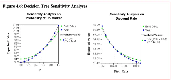
Figure 4.6: Decision Tree Sensitivity Analyses ……… 40
Figure 4.7: Geometric Brownian Motion of Asset Price ………..……… 52
Figure 4.8: Binomial Tree with Asset Prices (P) and Call Option Payoff (C) ………..… 58
Figure 4.9: Valuing Land as an American Call Option using Binomial Tree ………..… 60
Figure 4.10: Monte Carlo Simulations for a simple development option ………..…………...… 61
Figure 4.11: Underlying Asset and European Call Value Distributions from Simulation …...… 63
Figure 4.12: Multi-Phase Development Project as Sequential Compound Option …………..… 66
Figure 4.13: One Year Asset Price Movement ………...………..… 72
Figure 4.14: Decision Tree Version of Development Option ……….…..… 72
Figure 5.2: Project Company Structure ……… 82
Figure 5.3: Summary Income Statement and Balance Sheet of POSCO E&C ……… 83
Figure 5.4: Top 10 Foreign Banks in Korea ………. 85
Figure 5.5: Phase 1 Project Inventories ……….... 86
Figure 5.6: For-Sale Properties Costs and Profit Analysis ………... 87
Figure 5.7: Income Properties Costs and Return Analysis ………...… 88
Figure 5.8: Pro-forma Project Level Annual Cash Flow ………..… 89
Figure 5.9: Incheon Free Economic Zone Metropolitan Infrastructure Plan ……… 92
Figure 5.10: World Trade and Convention Center Complex ……… 95
Figure 5.11: Development Map of New Songdo City ……….. 97
Figure 5.12: Typical Condominium Payment Schedule ………... 99
Figure 5.13: Short and Long-Term Financing Analyses for First Phase ……… 100
Figure 6.1: Summary of Project Inventories ………...……… 103
Figure 6.2: Korean Stock and Housing Market (1993-2003) .……… 104
Figure 6.3: Residential Sales Price and Chonsei Deposit Index (1993-2003) ……… 105
Figure 6.4: Office Vacancy Rates, Seoul (1993-2003) ………...……… 106
Figure 6.5: Office Sales Price and Rent Index, Seoul (1993-2003) …...……… 107
Figure 6.6: New Songdo City Construction Schedule ………...……… 109
Figure 6.7: 3-Year Korean Government T-Bill Rates (1994-2003) …...……… 110
Figure 6.8: Annual Changes in GDP and CPI (1993-2003) …………...……… 110
Figure 6.9: Input Assumptions for DCF Analysis ...………...……… 111
Figure 6.10: Summary of NPV analysis based on DCF method ……....……… 111
Figure 6.11: Monthly Return Volatility of Construction Companies and Residential Sales Prices ………114
Figure 6.13: Sensitivity of Option Value on Volatility (σ) and Asset Value (S) ……… 119
Figure 6.14: Option Value Sensitivity Graph ..………...……… 120
Figure 6.15: Structure of Decision Tree for Analysis of Project Specific Risks ……… 122
We do ten-year pro-forma cash flow analysis but we don’t really believe in them.
Who knows what’s going to happen down on the road?1
Nobody really uses IRR or NPV within the development industry. It’s just for institutional equity investors … [Therefore,] non-institutional investors are
preferable for us. They are mostly interested in cash on cash returns.2
Three methods mentioned above – Discounted Cash Flow (DCF), Net Present Value (NPV) and Internal Rate of Return (IRR) – have been widely accepted tools for any investment analysis. Yet, a number of anecdotal evidences suggest that real estate developers find these tools insufficient for the analyses of their development projects. The entrepreneurial nature of the development industry might have contributed to this lack of rigorous analyses: So called developers’ gut-feelings sometimes become more important factors to the decision making process. However, it has been proven that DCF, NPV and IRR with a hurdle rate are fundamentally sound tools, and even within the real estate industry, these are standard methods for valuing income-generating institutional properties. In this sense, the relatively limited use of DCF based analyses in the development industry does not seem to be entirely due to developers’ naïveté. The true reason for their limited use might be their failure to capture a part of everyday reality involved with typical development projects.
I believe that the inadequacy of conventional DCF, NPV and IRR for a development project analysis originates from their very static nature of underlying assumptions. On the contrary, the
1 From the presentation by the CEO of a leading New York development firm at MIT.
essence of most development projects is their dynamic processes. Conventional methods give a single point estimates based on all the information available, and thus, it inherently implies that all the investment decisions are made as of now (time 0). Since most investment decisions for development projects are made in sequence over some time period, the conventional methods fail to incorporate flexibility of future decisions. This flexibility is all the more critical for large-scale urban mixed-use projects with multiple stages over time, and a static DCF based analysis would grossly misrepresent merits of such large scale projects.
The goal of the thesis is to evaluate and apply methods for incorporating flexibility into the analysis of large-scale real estate development projects. The first half of the thesis attempts to layout theoretical framework for evaluating complex development projects, first using NPV approach and later extending NPV analysis with Decision Tree Analysis and Real Options. The second half of the thesis is a case study applying the methods developed in the earlier chapter to the “New Songdo City (NSC)” project in Incheon, Korea. The NSC project is a highly complex new city development project that involves 100,000,000 square feet of building space and 12 year project schedule with 6 different phases. The rather simplified application of Decision Tree and Real Options analysis demonstrate the reason why the concept of flexibility and option is critical for such a large scale project with a high level of uncertainties, and at the same time, reveals some difficulties in applying options model to real world practices.
Ch. 2. Literature Review
The thesis deals with two methodologies – Decision Tree Analysis and Real Options Analysis – as tools for valuing flexibilities inherent in large-scale real estate development projects. Real estate development projects, unlike buy-sell decisions made for investing in pre-existing assets, require series of decision making over time, and for each future decision there are numbers of alternatives available. Therefore, it is important to identify what alternative courses are available and to plan ahead the best course of action given the flexibility. Decision Tree Analysis is a useful tool for laying out alternative courses of actions and their corresponding future payoffs. The use of Decision Tree was first advocated by J. Margee (1964) as a tool for corporate capital planning. Brealey and Myers (2003) introduced Decision Tree to illustrate how managerial flexibilities can create value for a capital project. They went one step further to propose a valuation technique under the Decision Tree structure. At the same time, they identified
difficulties of determining a proper discount rate and probabilities. De Neufville (1990) proposed to use Decision Tree for finding optimal strategies for complex engineering projects. The
application of Decision Tree Analysis to real estate projects has been limited, and there has been little research done for this purpose. However, the method is very relevant for real estate projects as demonstrated in the chapter 4, and it is safe to assume that it has been implicitly used for real estate decision makings.
Real Options, on the other hand, has been studied frequently and rigorously by academics, and there have been a number of researches done for its application to the real estate industry.
Recently, many academics and practitioners attempted to apply options valuation techniques to real world projects and investments. Arman and Kulatilaka (1999); Copeland and Antikarov (2001); and Mun (2002) promoted the use of the binomial tree approach in conjunction with Decision Tree to identify and value Real Options on real world projects in a practical manner. Dixit and Pindyck (1994) followed more theoretical approach by developing a series of mathematical models for the purpose of applying them in the real world.
Real Options Analysis is useful for the analysis of real estate projects due to the fact that various options are embedded in them. Titman (1985) first identified a vacant land as an option to buy a stabilized property at an exercise price equal to its construction costs. Through the application of the options theory, he explained the relationship between building activity and uncertainty. He argued that increased uncertainty led to a decrease in building activity in the current period. Williams (1991) constructed an options model of real estate development to analyze the optimal timing and the scale of a development. Capozza and Sick (1991) explained the difference in value between leased and fee-simple3 property with a redevelopment options model. Based on their model, the discounts on leased properties are larger with high conversion efficiency, low interest rate, high growth rate or high uncertainty.
Flexibility in land use choice has been analyzed using the options valuation theory. Capozza and Helsley (1990) developed a land price model based on uncertain household income and land rent. This model predicted that the effect of uncertainty would delay the conversion of agricultural land to urban land; reduce expected city size; and impart an option value to agricultural land. Geltner et al (1996) examined the option that is present when a site for development has more than one allowable uses. Based on the authors’ model that values the options to choose to construct one of two uses, they found that this option could add as much as 40% to the land value. This option to
choose adds the most value when the cost of land is low relative to construction costs. The model also identifies that the conditions for optimal development of the land become more difficult to achieve, and furthermore, development would never occur when the two land use choices have equal value. Childs et al (1996) examined the options related to the mixed-use projects. They came up with a model that incorporates an option to mix two uses on a site and also a redevelopment option. Their model suggests that returns become less certain and uses less correlated as the option to redevelop increases in value. The model also predicts that mixed-use developments will be more common in markets that are more supply sensitive or when the project is large relative to the existing supply.
There have been many attempts made to explain aggregate level real estate market behaviors with Real Options framework. Williams (1993) pointed out the differences between financial options and Real Options in real estate projects, and modeled developers’ behaviors. According to him, options on real estate differ from financial options in that each real asset produces goods or services with a finite demand elasticity; all options to develop cannot be exercised simultaneously due to the limited capacity of developers; and the supply of undeveloped assets is limited. Based on these assumptions, the model predicted that development is optimal at all values above a critical value. Thus, below this optimal value, no developer builds, and above the optimal value, all developers build at the maximum feasible rate. Grenadier (1955) studied overbuilding
tendencies in real estate markets with an options model. He showed increase in construction time, cost of changing occupancy rates, or demand volatility would lead to overbuilding. Grenadier (1996) later went once step further to explain the overbuilding tendency by incorporating the game theory approach. He argued that the simultaneous exercises and development cascades might be resulted from the rational fear of preemption rather than irrational overbuilding. Li (1999) developed a model to explain land development in emerging markets where newly developed properties account for a substantial portion of the aggregate supply of such properties.
By incorporating demand elasticity, the model suggested that the value of land and developed properties in the emerging markets were much lower than the corresponding values in the markets with perfect demand elasticity. It also illustrated that the optimal intensity and the land value were most sensitive to market demand conditions when interest rates and construction costs were lowest.
There also has been some empirical research conducted to find evidences of real options pricing in real estate and other markets. Quigg (1993) examined land transaction data in Seattle and compared actual transaction prices with implied residual values of land. She found out that market land prices showed average 6% premium of optimal development over the residual value. This finding demonstrated that market participants indeed value options of waiting for optimal development. Holland, Ott and Riddiough (1999) proposed a model to test neoclassical versus option-based model of investment against US commercial real estate data. They found that the evidence favors the option-based model over the neoclassical model with respect to total
uncertainty and thus irreversibility and delay are important aspects to investment decision-making. Another interesting result from their test was that short-run supply was inelastic with respect to changes in asset price but highly elastic to changes in price uncertainty. They suggested, in real asset markets, information regarding changes in price volatility might be more useful than information on changes in price levels.
Several empirical researches were also conducted for non-US markets. Yamaguchi et al (2000) applied a real options model similar to the one developed by Quigg to Tokyo real estate market data. They found out that the options premium for vacant land in Tokyo were average 18% over residual value. This was much higher than Quigg’s estimation of 6% premium of the Seattle market, and it might be due to the high level of speculative activities in Tokyo. Bulan, Mayer and
estimate the value of waiting for optimal development. Their study suggested that builders delayed development during times of greater uncertainty in real estate returns and when the exposure to market risk was higher. They also showed that competition significantly reduced the sensitivity of option exercise to volatility. Therefore, competitive firms were not able to capture the full benefits to waiting that a monopolist had. Based on their case studies on residential development projects, Yao and Pretorius (2004) argued that the Hong Kong government was undervaluing land that it provided to developers because the government used the conventional DCF valuation method. They suggested the Hong Kong government use the Real Options approach to increase revenue and alleviate its fiscal constraints.
The literature on developing Real Options model for real estate markets has been increased dramatically in recent years. The validity of options model in real estate was also tested and confirmed through empirical testing by academics, which some of them are mentioned above. However, the focus has been given to developing mathematical and statistical models, and there has been little attempt made to developing a Real Options method that could be easily applied by average practitioners. The concepts and procedures involved with the most Real Options models are beyond the scope of average practitioners’ knowledge of the subject, and therefore, the application of Real Options Analysis to real estate development projects has been limited. The empirical studies, however, shows that the development industry implicitly takes advantage of the options inherent to development projects. Thus, It is crucial to strategically use options in real estate developments to become a successful developer. In this context, this thesis aims to implement practical methods to incorporate flexibilities and options inherent during real estate development processes, using Decision Tree and Real Options Analysis.
Ch. 3. Discounted Cash Flow based Analyses of Real Estate
Development Projects
3.1. Fundamentals of Net Present Value and Internal Rate of Return Methods
Discounted Cash Flow (DCF) methods have traditionally been a fundamental principle in business decisions where money is invested now for yielding future returns. The basic principle of any DCF analysis is that expected future returns need to be “discounted” with an appropriate risk adjusted discount rate. Two of the most common DCF methods are Net Present Value (NPV) and Internal Rate of Return (IRR) (Hammond III, 1975).
The NPV analysis basically asks whether a project is worth more than its costs. Intuitively, if benefits of a project exceeds or is at least equal to its costs, the project is worth undertaking. The essence of the NPV analysis is estimating what benefits and costs are worth for investors. The conventional NPV analysis applies a discount rate, determined by the concept of opportunity cost of capital, to value costs and benefits in present terms (Brealey and Myers, 2003). For a simple investment that requires the initial cash investment of C0 with T year life, the NPV for the project can be calculated as follows:
T T
r
C
r
C
r
C
C
NPV
)
1
(
)
1
(
1
2 2 1 0+
+
+
+
+
+
+
=
K
Here, r is the opportunity cost of capital for the given project, which should reflect risks of future cash flows. Based on this framework, the following investment decision rules are applied for a NPV analysis (Geltner and Miller, 2001):
• Maximize the NPV across all mutually exclusive alternatives.4
• Never choose an alternative that has a negative NPV.
The IRR analysis is another version of applying the concept of NPV. The IRR is defined as the rate of return that makes the NPV of a project equal to zero. By solving the following equation, we can find IRR for a project that lasts T years and requires the initial investment of C0 (Brealey and Myers):
0
)
1
(
)
1
(
1
2 2 1 0+
+
+
+
+
+
+
=
=
T TIRR
C
IRR
C
IRR
C
C
NPV
K
The actual calculation of IRR would involve trial and error. However, we can easily get the solution using IRR function in any common spreadsheet software. The IRR in itself is not as useful as the NPV analysis since it does not provide any information regarding the risk of the project. The IRR analysis only becomes useful when it is used in relation to the opportunity cost of capital – the required return of the project. Comparing the IRR with the required return is similar to the NPV analysis. That is, when the IRR is higher than the required return, the project would have a positive NPV. Following this method, the decision rule for the IRR analysis is (Geltner and Miller):
• Maximize the difference between the project’s expected IRR and the required return.
• Never do a project with an expected IRR less than the required return.
4 In principle, this rule should factor in all alternatives including flexibilities of delaying, abandoning, etc.
Therefore, options value should be considered for NPV maximization (similar to the concept of eNPV that will be introduced in the chapter 4). However, in practice, NPV is only calculated using the static DCF procedure, and thus leaves out any potential value of flexibility. In this context, the thesis does not attempt to replace the NPV decision rule but rather aims to expand the conventional NPV procedure to incorporate the value of flexibility.
3.2. Application of DCF based analysis to Real Estate Development Projects
As illustrated in the previous chapter, the key element in the development of the NPV and the IRR methodology is the identification of r, known as discount rate or opportunity cost of capital. In theory, a discount rate should be same as the rate of return of equivalent investment
alternatives in the capital market. Fortunately, the real estate industry has a very active market, and it is possible for investors to estimate a real asset’s opportunity cost of capital by observing the market. Although the real estate market is not as efficient as the security markets due to the uniqueness of individual real assets and the infrequent trading, it is possible to find out the fairly reliable opportunity costs for a stabilized building investment. When applied to the investment analysis for a core stabilized asset, the NPV and the IRR have been proven effective.
In contrast to existing properties, the required return for development projects is not easily observable from the market. This might be one reason why the NPV approach is not as popular in the development industry. It is reasonable to assume that development projects are much riskier and thus require higher return. Furthermore, development projects are unique in that they involve multiple distinct phases. For instance, a development process typically involves buying an undeveloped land, permitting, construction, lease up, and stabilization. Each phase in a
development process has a distinct level of risk. Therefore, to be consistent with the underlying theory, cash flows from each phase need to be discounted with its own risk adjusted discount rate.
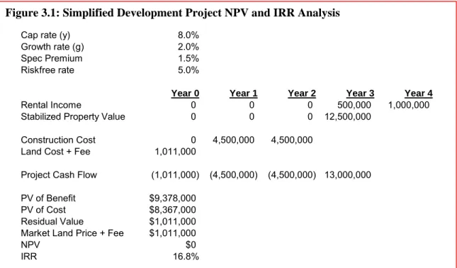
Consider a development project for a land valued at $ 1,900,000. In addition to the land value, there is $ 40,000 of permitting related costs incurred at the time zero. The best use for the site is building an office building, and it is expected to generate an annual net operating income of $ 1,000,000. The lease-up is estimated to take about a year and it would generate $500,000 during the period. The cap rate of 8% and the opportunity cost of 10% are estimated for investing a
similar office building that the developer proposed to build. For speculative buildings, the
additional 1.5% of premium can be reasonably assumed based on the market analysis. The annual income growth is expected to be 2%. The construction is estimated to cost $ 8,000,000 over two years with equal amount spent in each year. Figure 3.1 illustrates the annual cash flow of this development project.
In this example, there are two types of future expected cash flows. One is the construction cost cash flow and the other is the future income cash flow. As Brealey and Myers explained in their analysis of the Mark II investment, fixed future cash flows should be discounted with a risk free rate. On the other hand, the discount rate for the future incomes can be obtained from the market, and in this case, the lease-up phase discount rate of 11.5% can be used. Based on this information, the following NPV principle can be used for the development project:
)
(
)
(
)
(
Developmen
t
PV
0Benefits
PV
0Costs
NPV
=
−
Assuming the building would be stabilized in the year 4, we can calculate the value of the
building as of the year 3 with the stabilized discount rate of 10% and the long-term growth rate of 2%:
000
,
500
,
12
02
.
0
1
.
0
000
,
000
,
1
)
(
3Stablized
−
Office
=
−
=
PV
Using the lease-up discount rate of 11.5%, the present value of benefits is calculated:
000
,
378
,
9
115
.
1
000
,
500
,
12
115
.
1
000
,
500
)
(
3 3 0Benefits
=
+
=
PV
The present value of costs can be calculated in the same manner using the discount rate of 5% and the land cost at the time zero:
000
,
378
,
9
05
.
1
000
,
450
05
.
1
000
,
450
000
,
011
,
1
)
(
2 0Costs
=
+
+
=
PV
Since the benefits and the costs are equal, the NPV of this development project is zero. Unless there are other opportunities with a positive NPV, the project is worth undertaking based on the NPV decision rule.
The method presented above is a theoretically sound from the NPV perspective. However, it displays several disadvantages. The IRR of the project is 16.8% based on the cash flow projection in the figure 3.1. The IRR supposedly reflect higher risk of speculative development projects and indicates the risk premium of 6.8% over the required return of 10% for the stabilized buildings. However, it is hard to value the 6.8% premium because it is a blended rate of two distinct phases of construction, lease-up and stabilized operation. Therefore, in practice, it can be more helpful to identify the development period return in isolation. Geltner (2002) proposed a method to calculate the development required return based on the equilibrium across the markets related to the
development industry. Since we already can reasonably estimate risks of stabilized assets and construction debts, we can calculate risks of development based on the other assets. That is, a development investment is equivalent to having a long position in the stabilized property and a short position in the construction costs at the same time. Assuming markets are efficient, this long
Figure 3.1: Simplified Development Project NPV and IRR Analysis
Cap rate (y) 8.0%
Growth rate (g) 2.0%
Spec Premium 1.5%
Riskfree rate 5.0%
Year 0 Year 1 Year 2 Year 3 Year 4
Rental Income 0 0 0 500,000 1,000,000
Stabilized Property Value 0 0 0 12,500,000
Construction Cost 0 4,500,000 4,500,000
Land Cost + Fee 1,011,000
Project Cash Flow (1,011,000) (4,500,000) (4,500,000) 13,000,000
PV of Benefit $9,378,000
PV of Cost $8,367,000
Residual Value $1,011,000
Market Land Price + Fee $1,011,000
NPV $0
and short position must be equal to the development project, and thus the following relationship can be assumed:
(
)
(
) (
)
T D T T V T T C T Tr
E
L
r
E
V
r
E
L
V
]
[
1
]
[
1
]
[
1
+
=
+
−
+
−
TV = Expected value of stabilized property at time T T
L = Expected balance due on construction loan at time T
]
[
r
VE
= Market required return on investments in a stabilized property] [rD
E = Market required return on construction loans
Based on this relationship, we can estimate the required return for the development period:
(
)(
) (
)
(
)
(
)
( )1
]
[
1
]
[
1
]
[
1
]
[
1
]
[
1−
⎥
⎦
⎤
⎢
⎣
⎡
+
−
+
+
+
−
=
T T T V T T D T D T V T T CL
r
E
V
r
E
r
E
r
E
L
V
r
E
Using the proposed method, the development period return of 48.5% is calculated. This method identifies development risk as a separate risk regime by standardizing the development as a two period process and it can be more easily compared with other projects. Also, the required return here is calculated without knowing the value of the land, and as a result, it gives information as to what price investors should pay for the land for a positive NPV development project. Figure 3.2 illustrates the procedure to get the development return based on the analysis performed in Figure 3.1. This clearly shows that the project is NPV positive when the land can be acquired for less than $1,011,000.
Figure 3.2: Estimation of Two-Period Development Required Return
Year 0 Year 1 Year 2 Year 3
Value of Stabilized Office at T=3 13,000,000 Value of Const. Cost at T=3 9,686,250
NPV at T=3 3,313,750
Residual Value at T=0 1,011,000
Two Period Cash Flow (1,011,000) 0 0 3,313,750
The two methods presented above provide a sophisticated analytical framework to analyze development projects based on NPV and DCF. However, the model’s usefulness depends on how effectively it can help the real world decision making process. Development projects, unlike typical investments in pre-existing assets or securities, involve sequential cash outflows over time. Accordingly, valuing the cost side of the NPV becomes as important as the benefit side. In other words, in addition to the risks of receiving future incomes, development projects deal with the risks related to the costs, such as construction cost overruns and construction delays. Therefore the question is whether the previously used methods reflect all the risks related to the
development stage. From the theoretical perspective, the development stage required return should capture these development risks. When applied in practice, the previous models exhibit a high degree of sensitivity to variations in underlying assumptions.
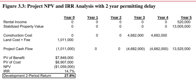
Figure 3.3 shows changes in NPV and returns when there has been 2 year delay in permitting with otherwise identical cash flow as in Figure 3.1. These kinds of delays and changes are rather norm than exception in most development projects, and thus, it is fair to say the model’s
usefulness depends on its ability to deal with future changes. The 2 year delay in permitting as illustrated in Figure 3.3 result in 2.1% decrease in the going-in IRR and 20.7% decrease in the development two-period return. Also, as shown in Figure 3.4, 10% decline in the expected asset price would result in 7% decrease in the going-in IRR and 22.7% decrease in the development
Figure 3.3: Project NPV and IRR Analysis with 2 year permitting delay
Year 0 Year 1 Year 2 Year 3 Year 4 Year 5
Rental Income 0 0 0 0 0 520,000
Stabilized Property Value 0 0 0 0 0 13,005,000
Construction Cost 0 0 0 4,682,000 4,682,000
Land Cost + Fee 1,011,000
Project Cash Flow (1,011,000) 0 0 (4,682,000) (4,682,000) 13,525,000
PV of Benefit $7,848,000
PV of Cost $8,907,000
NPV ($1,059,000)
IRR 14.7%
return. The higher degree of development projects’ sensitivity comes from the fact that they are levered positions on stabilized properties. That is, the upfront purchase of land brings with it the operating leverage, which is project exposure to fixed costs (Brealey and Myers).
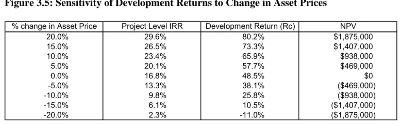
Figure 3.5 illustrates sensitivity of the exemple project in Figure 3.1 to the variation of the stabilized asset price. These example cases illustrate that, although the higher required return for development projects might compensate for their higher risks, the NPV and the required return based analyses does not help developers strategically dealing with the risks. To be sure, the NPV analysis is useful for avoiding bad projects and comparing with alternative projects with some standard measure. However, unlike investment decisions for stabilized assets, decisions regarding development projects are typically made over time, as cash outflow occurs over the time of the development. In this regard, for developers in practice, a tool to help them think ahead of future
Figure 3.5: Sensitivity of Development Returns to Change in Asset Prices
% change in Asset Price Project Level IRR Development Return (Rc) NPV
20.0% 29.6% 80.2% $1,875,000 15.0% 26.5% 73.3% $1,407,000 10.0% 23.4% 65.9% $938,000 5.0% 20.1% 57.7% $469,000 0.0% 16.8% 48.5% $0 -5.0% 13.3% 38.1% ($469,000) -10.0% 9.8% 25.8% ($938,000) -15.0% 6.1% 10.5% ($1,407,000) -20.0% 2.3% -11.0% ($1,875,000)
Figure 3.4: Project NPV and IRR Analysis with 10% asset price decline
Year 0 Year 1 Year 2 Year 3 Year 4
Rental Income 0 0 0 450,000 900,000
Stabilized Property Value 0 0 0 11,250,000
Construction Cost 0 4,500,000 4,500,000
Land Cost + Fee 1,011,000
Project Cash Flow (1,011,000) (4,500,000) (4,500,000) 11,700,000
PV of Benefit $8,440,000
PV of Cost $9,378,000
NPV ($938,000)
IRR 9.8%
decisions and their impact on the project would be much more meaningful than the NPV analysis based on a decision at the time zero.
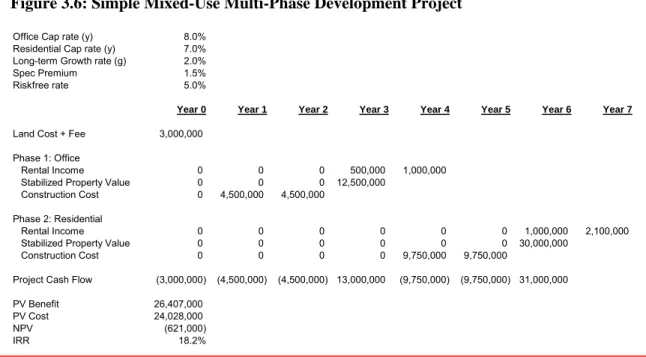
For large-scale projects with extended development period and multiple stages, the sensitivity of the NPV and the required return based analyses to underlying assumptions becomes magnified. Consider a mixed use development project with the following characteristics:
• Current market value of the land is $2,700,000. The upfront fee of $300,000 is required for design and permitting. Out of $3,000,000, $1,011,000 is attributable to the office component, and the remainder is attributable to the residential component.
• According to the current zoning regulations, one office building and one residential building can be built on site. The office building can be developed immediately. However, it would take up to 3 years for the residential building to break grounds due to the likely permitting complications.
• The construction of the office building is expected to take 2 years. The total cost is estimated to be $9,000,000, with two equal payments of $4,500,000 each year during the construction.
• The office building is expected to generate an annual income of $1,000,000, when stabilized in the year 4. The lease-up would take about one year with $500,000 generated during the period.
• The construction of the residential building is also expected to take 2 years. The total cost is estimated to be $19,500,000, with two equal payments of $9,750,000 each year during the construction.
• Based on the market research, the cap rates for the office and the residential properties are 8% and 7% respectively. For the appropriate discount rates, the growth rate of 2% and the spec premium of 1.5% will be added to the market cap rates.
Given the above information, it is possible to perform a NPV analysis of the project. Using the same method as in Figure 3.1 – Discounting costs with free rate and benefits with risk-adjusted rate – , the resulting NPV of the project is negative $621,000 as shown in Figure 3.6. Following the NPV decision rule, the project should be rejected. Even though this multiple phased project has a higher project level blended IRR than the single asset development in Figure 3.1, it is quite inferior project based on the NPV. This result demonstrates that the longer
development period and related uncertainties require higher return due the additional risks involved. Accordingly, the project’s negative NPV seems well justified. However, given the sensitivity of the development project’s NPV, the further test of the analysis should be granted.
Figure 3.7: Sensitivity of Multiple Phase Project to Change in Asset Prices
% change in Asset Price Project Level IRR NPV
20.0% 28.6% $4,661,000 15.0% 26.1% $3,340,000 10.0% 23.6% $2,020,000 5.0% 20.9% $699,000 0.0% 18.2% ($621,000) -5.0% 15.3% ($1,941,000) -10.0% 12.3% ($3,262,000) -15.0% 9.2% ($4,582,000) -20.0% 5.9% ($5,902,000)
Figure 3.6: Simple Mixed-Use Multi-Phase Development Project
Office Cap rate (y) 8.0% Residential Cap rate (y) 7.0% Long-term Growth rate (g) 2.0% Spec Premium 1.5% Riskfree rate 5.0%
Year 0 Year 1 Year 2 Year 3 Year 4 Year 5 Year 6 Year 7
Land Cost + Fee 3,000,000 Phase 1: Office
Rental Income 0 0 0 500,000 1,000,000 Stabilized Property Value 0 0 0 12,500,000
Construction Cost 0 4,500,000 4,500,000 Phase 2: Residential
Rental Income 0 0 0 0 0 0 1,000,000 2,100,000 Stabilized Property Value 0 0 0 0 0 0 30,000,000
Construction Cost 0 0 0 0 9,750,000 9,750,000
Project Cash Flow (3,000,000) (4,500,000) (4,500,000) 13,000,000 (9,750,000) (9,750,000) 31,000,000 PV Benefit 26,407,000
PV Cost 24,028,000
NPV (621,000)
The sensitivity analysis to the asset price change in Figure 3.7 shows that there are huge down sides from the base scenario and yet only 5% higher asset price would move the project into the positive NPV realm.
Since this project has multiple components in it, it is useful to analyze each component
individually to identify which one loses (gains) most value. As shown in Figure 3.8, it turns out that the office component has zero NPV, whereas the residential component loses all the value mostly due to the fact that it is planned to begin construction three years later. That is, the negative impact on the NPV would be greater with later stage projects as costs are discounted with a much lower rate than benefits. In fact, if the construction can begin at the year 1, the residential component would generate $2,858,000 of positive NPV, which is much greater than the office component would generate. Due to the procedure that requires much higher discount rate for benefits than one for costs, the later projects are always less desirable compare to the earlier ones from the NPV standpoint, even if they are similar in all the other aspects. This might be one of the reasons why developers often times favor Cash-On-Cash return over NPV or IRR. From the example, the office building and the residential building each has 39% and 54%
Figure 3.8: NPV Breakdown of Multiple Phase Project
Year 0 Year 1 Year 2 Year 3 Year 4 Year 5 Year 6 Year 7 Phase 1: Office
Rental Income 0 0 0 500,000 1,000,000 Stabilized Property Value 0 0 0 12,500,000
Construction Cost 0 4,500,000 4,500,000 Land Cost + Fee 1,011,000
Office Cash Flow (1,011,000) (4,500,000) (4,500,000) 13,000,000 Office IRR 16.8%
PV of Office Income Flow 9,378,000 PV of Office Cost 8,367,000
Office NPV 0
Phase 2: Residential
Rental Income 0 0 0 0 0 0 1,000,000 2,100,000 Stabilized Property Value 0 0 0 0 0 0 30,000,000
Construction Cost 0 0 0 0 9,750,000 9,750,000 Land Cost + Fee 1,989,000
Office Cash Flow (1,989,000) 0 0 0 (9,750,000) (9,750,000) 31,000,000 Office IRR 18.9%
PV of Residential Income Flow 17,029,000 PV of Residential Cost 15,661,000 Residential NPV (621,000)
Cash-On-Cash return respectively.5 Evidently, Cash-On-Cash return is not a theoretically sound measure because it does not account for any risks or time factor. However, the NPV analysis clearly penalizes later stage projects and discourages any long-term commitment on large-scale developments. This problem calls for improved analytical tools for valuing long-term
development projects.
3.3. Shortcomings of Discounted Cash Flow based Analyses
As identified in the previous analyses, the NPV and IRR analyses work well for the valuation of a project based on a single fixed assumption. However, they are not as useful for real estate
development projects, due to flexibility in subsequent decisions. Simply requiring higher returns for their higher risks does not help much in practice, although it might guide developers to weed out poor projects. The shortcomings of DCF based analyses originate from their fundamental assumptions. According to Copeland and Keenan (1998a), DCF techniques were developed to value investments such as stocks and bonds, and their basic assumption is that investors hold them passively. Thus, DCF based models like NPV overlook investors’ capabilities of future decision making to alter the original course of a project in response to any future changes. In fact, they assume that investors make all the decisions based on their future expectations at the time, and then later they do not deviate from the initial decisions made.
De Neufville (1990) goes further to say that the conventional DCF analysis fails to recognize the fact that managers manage projects. According to him, this is the critical flaw of the DCF analysis.
5 Cash-on-Cash return is calculated without any consideration for discount factor. It can formally expressed
as: Cash-on-Cash return = (Built Asset Value – Construction Costs)/Construction Costs = Development Profit Margin / Construction Cost. For example, office Cash-on-Cash return = (12,500,000 – 9,000,000) / 9,000,000 = 38.9%.
The DCF procedures assume a single line of development for a project so that a project is carried through even if it fails. The analysis simply incorporates the probability of failure into the overall expectation of the project.
These flaws of the DCF based analyses are crucial to the analysis of real estate development projects, because the decisions related to development projects are spread over the entire development period and this give a greater degree of flexibility to adapt to any future changes. That is, large-scale development projects are rarely executed as they were planned initially. I would argue that the success of any development project depends heavily on the strategic use of flexibilities imbedded in the project.
Ch. 4. Valuing Flexibility in Real Estate Development Projects
4.1. Decision Tree Analysis (DTA)
Decision Tree Analysis (DTA) is one of the important tools available that takes flexibilities – left out from the NPV analysis – into account. It was first advocated by J. Magee in 1964 and has remained an important tool for capital investment decisions. DTA is basically a tool that can depict strategic future pathways an investor can take based on a number of different future outcomes. It shows graphically a decision road map of an investor’s and manager’s strategic initiatives and opportunities over time. DTA can be used when future outcomes are uncertain and investors have tool to react when new information is arrived in the future.
Prior to exploring DTA in detail, it is necessary to examine the concept of the expected return, which is basis of the conventional DCF analysis. According to Bodie et al (2002), the expected return of an asset is a probability-weighted average of its return in all future scenarios. Let Pr(s) be the probability of scenario s and r(s) be the return in scenario s, the expected return .E(r) can be expressed as:
∑
⋅
=
ss
r
s
r
E
(
)
Pr(
)
(
)
For example, consider the return for a downtown office building that is sensitive to the overall regional economy. For the sake of the analysis, we can assume the following scenario for the next year:
Bullish Economy Bearish Economy Economic Crisis
Probability .4 .4 .2
Return 30% 10% -30%
Applying these values to the formula defined above, the expected return of the office building is:
=
−
×
+
×
+
×
=
(.
4
30
)
(.
4
10
)
(.
2
(
30
))
)
(
r
officeE
10%The conventional NPV method blindly uses this 10% as the basis of the investment analysis. However, it is critical to note that for actively managed investments like real estate development projects, managers can take action to prevent losses when the future outcome turns adverse. The main idea of DTA is to map out potential decisions so that it would enhance future outcome of a project. If an investor acquires an option to buy the office building, instead of buying the office immediately, she would not exercise option for a loss. Therefore, the investor’s average return would be – without considering the option price and the lost time value of delaying the commitment:
%
16
)
0
2
(.
)
10
4
(.
)
30
4
(.
)
(
r
office.w.option=
×
+
×
+
×
=
E
As shown, the ability to make decisions when future outcome is known creates value to a project. DTA is designed to help investor to maximize the benefit of the sequential decision making.
Decision Tree Analysis incorporates the value of flexibility by explicitly laying out the structure of a project in such a way that all uncertainties and the potential decisions to be made on the uncertainties are represented as a tree form. According to de Neufville (1990), DTA leads to the following three results:
• Structures the problem, which otherwise would be very confusing due to the complexities introduced by uncertainty.
• Defines optimal choices for any period through an expected value calculation based on the consideration of the probabilities and the outcomes of each choice.
• Identifies an optimal strategy over many periods of time.
These benefits of DTA can be used to correct shortcoming of the DCF-based analyses as previously identified. DTA illustrates how future decisions could be made as uncertainties regarding a project reveal themselves over time. Therefore, it does not assume pre-committing all the decisions at the time zero. Unlike the NPV analysis, DTA assumes that investors will learn new information about the project and they have flexibilities to change course of action as the project proceeds.
Following de Neufville’s approach, a Decision Tree is composed of three basic nodes:
• Decision nodes (square), where possible decisions are contemplated and a decision made.
• Chance nodes (circle), where outcomes are determined by events or states of nature.
Chance nodes have probability of each chance happening, and the sum of the probabilities in each chance node equals one.
• Terminal nodes (triangle), where a project is completed or abandoned. They are the end
points of the decision tree branches, and they are typically accompanied by terminal value of the path.
In its most basic form, a Decision Tree has series of decision nodes and chance nodes branching out to form a tree shaped structure. By assigning probabilities in chance nodes and terminal payoffs at the terminal nodes of each branch, it is possible to value the project at each decision node. Described formally, the expected value of a risky decision Di is the outcomes weighted by their estimated provability of occurrence:
ij j j i
P
O
D
EV
(
)
=
∑
⋅
When there are a number of alternatives choices to be made, the decision rule in DTA is to choose the one that offers the best average value, defined as the expected value (EV) above. When multiples nodes and branches are involved, EV is calculated backwards from the terminal
nodes to the initial node. The following is a simple example of the decision tree regarding an investment decision:
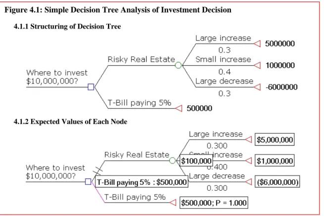
The simple analysis in Figure 4.1 identifies T-Bill as a superior investment than risky real estate, based on the expected value calculation6. This example is deterministic model in that it assumes all the future probabilities of outcomes are already known. It is possible to estimate probabilities and payoffs based on past data and experience, and it would not possible to know for sure in most cases. The real world application of Decision Tree Analysis would have much more complex form and involve numerous variables. The strongest virtue of DTA is that it exposes all the uncertainties and the accompanying flexibilities of a project wide open, which otherwise would have been treated as a “black box” that only gives a single value estimation.
6 The example in Figure 4.1 does not account for discount rate and time, and therefore does not factor in
investor’s risk aversion. In this case, the expected value of investing in risky real estate is lower despite the potentially greater risks, and thus investing in T-Bill obviously superior to real estate. Another way to incorporate risks in this framework would be using a risk adjusted probabilities so that the probability of each outcome is adjusted for the risk. However, it would be hard to implement this approach in practice due
Figure 4.1: Simple Decision Tree Analysis of Investment Decision
4.1.1 Structuring of Decision Tree
4.2. Application of Decision Tree Analysis to Real Estate Development Projects
As describe in the previous chapter, real estate development projects involve a sequential decision making as they progress. Therefore, they are ideal candidates for Decision Tree Analysis. A typical development project involves decisions on purchasing a piece of land, choosing a right program and capacity, choosing an optimal timing to build, etc. We can analyze office
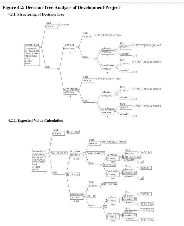
development project in Figure 3.1 using DTA. The previous analysis, fully committing to build an office building from the outset, resulted in zero NPV. It is important to note that the benefit side of the equation is highly uncertain, yet the costs side is relatively predictable. Thus, there is a value in waiting for higher benefits in the future. The current value of the asset to be developed is $9,378,000, which is the present value of future benefits. The cost of project is same as the current asset value, and it is composed of $1,011,000 of the land value and $8,367,000 of the construction costs. Figure 4.2 illustrates the decision tree that incorporates waiting up to 2 years7 before committing for the construction based on the following assumptions:
• There are two discrete possibility of future outcome in the office asset prices based on up market and down market.
• During the good market, the asset price will increase 22.1%, and during the down market, it will decrease 18.1%8.
• Probabilities of the up-market and the down-market are 60% and 40% respectively.
• Office would generate an annual income of 8% of its value. This would be lost income to the investor if she decides to wait for a better market.
7 Typical land development would have perpetual waiting option. However, this assumption is used for the
purpose of this decision analysis. Perpetual option on land will be examined in the next chapter.
8 Upward move and downward move of the asset price is estimated using the following formula based on
• An annual rate of 11.5% for an equivalent office building is used to discount future payoffs.9
9 This figure is for illustration purpose only and is not theoretically correct. Obviously, the discount rate for
development project should be higher than this. Discount rates for Decision Tree Analysis are investigated
Figure 4.2: Decision Tree Analysis of Development Project
4.2.1. Structuring of Decision Tree
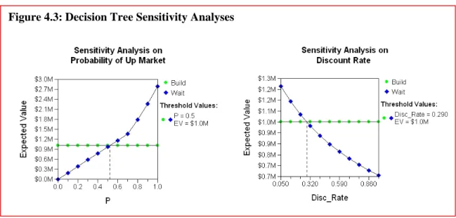
Bases on these assumptions, the DTA method reveals that there might be additional value in waiting for better outcome. However, the validity of this method is entirely dependent on the assumptions. More importantly, the probability and the discount rate are two most critical inputs in the model, yet entirely subjective numbers are used. Therefore, unless the assumptions are known for sure, a sensitivity analysis should be performed to see the robustness of the analysis and the boundaries of the decision rule. In figure 4.3, the lowest up-market probability for waiting decision to be optimal is 50% with the given discount rate. Also, with the 60% constant
probability of up-market, the highest discount rate for waiting decision to be optimal is 29%. These results can be compared to the market data, other similar type of development projects, or developers’ past experience to make more sensible judgment on the outcome of the analysis.10
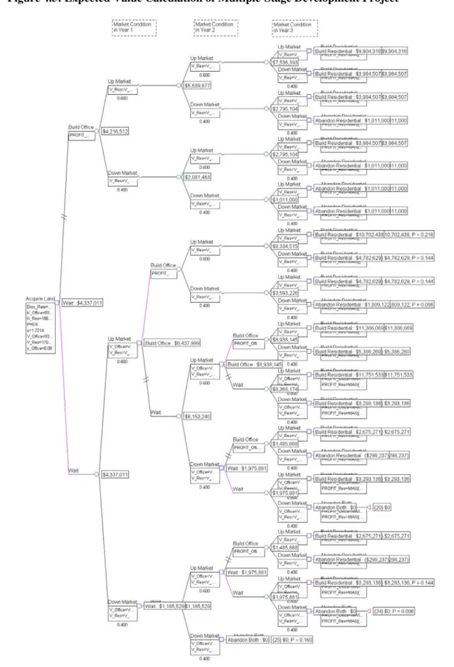
In the case of multiple-stage development projects, the decision tree analysis is even more useful due to the sequential decision nodes built in these projects. We can analyze the two-stage mixed use project from Figure 3.6 using DTA. Based on the previous NPV analysis, the project had the negative NPV of $621,000, and should be rejected based on the NPV decision rule. As the previous analysis revealed, the negative NPV was due to the second phase residential component,
10 More rigorous way to identify probabilities and discount rates is possible by using DTA in conjunction
with Real Options model. See the chapter 4.9 for details.
and the first phase, in fact, had zero NPV. Also the reason for the second phase’s negative NPV was mostly due to the conventional NPV procedures that assume the full commitment of all the components of the project at the beginning. The following rather simplified assumptions are made for the sake of a DTA analysis:
• The first phase office component can be built any time between the first year and the third year, and when the developer made commitment to build the office, she would have a right to build a residential building in the third year. For the sake of simplicity, the analysis assumes that the developer will decide whether to build the residential
component or not at the end of the third year (There is no more waiting option after the third year).
• Values of both office and residential properties are correlated with the market movement in that during an up-market asset price rises 22.1% and during a down-market, asset price falls by 18.1%.
• The office building would generate the annual income of 8% of its value and the lost income should be accounted for when the developer decides to wait for a better market.
• Probabilities of up and down-markets are estimated to be 60% and 40% respectively.
• 20% discount rate for the future profit is assumed by the developer.
Based on these assumptions, it is possible to map out the future market conditions and
accompanying strategies for the developer as in figure 4.4. Then, the Expected Value of the tree can calculated moving backwards from the terminal nodes. The calculations performed in figure 4.5 gives the expected value of $4,337,000. Since the land was purchased for $3,000,000, the NPV of the project becomes positive $1,337,000, which would be high enough to compensate for the initial negative NPV of $621,000. In other words, the value incorporating flexibilities outlined above is 83% higher than the value without any flexibility. The sensitivity analysis performed in figure 4.6 illustrates that, if the upside potential is greater than 50%, there is some value in
waiting for better market conditions. Also, with the 60% probability of up-market, the flexible strategy would be optimal with a discount rate lower than 33.3%. Precise value of the flexibility would depend on the reliability of the discount rate and the probability assumption. However, this simplified example demonstrates that it is essential to incorporate flexibility into the analysis of large-scale and multi-phase projects.
Another issue to be pointed out is related to the determination of the discount rate for each node. In this example, a single discount rate based on the developer’s subjective experience was used. However, it is evident that as the project progresses, the risk characteristic of the project also changes. In other words, real estate development projects are in part a learning process in that some future uncertainties become known as time passes. For example, once the developer knows that there were two consecutive up-markets, the payoff in the year three would be much less risky than when it was valued from the first year. Therefore, all the nodes in a decision tree would have different risk levels, and they should have corresponding discount rates. In realty, it is close to impossible to calibrate discount rates for each node, and for most cases, some degree of subjective judgment is required.
As shown in the previous two analyses, Decision Tree Analysis corrects the analysis performed using the NPV method by incorporating flexibilities of future decision makings. DTA should be used in conjunction with the conventional NPV method whenever there are flexibilities built in a project, especially when the project involves multiple stages. The NPV analysis would
systematically undervalue projects that have future phases of development, and without taking flexibilities into consideration, long-term projects would be rejected most of the time based on the NPV decision rule. However, DTA needs to be performed with much care to be an effective tool. Otherwise, it could lead to a distorted outcome and thus a poor investment decision. The
following chapter will examine shortcomings of DTA to aware of, for a better implementation of DTA.
4.3. Shortcomings of Decision Tree Analysis
Decision Tree Analysis is a great analytical tool that complements weaknesses of the
conventional Discounted Cash Flow based tools. Compared to the passive investment approach of the NPV analysis, DTA is much closer to the reality of actively managed real estate development projects. However, DTA has its own shortcomings and they should be clearly identified and understood by investors to be implemented for real world projects. The problems of applying DTA have been identified by many authors including Meyers (2002) and de Neufville (1990).
As Meyers points out, the difficulty of DTA’s implementation comes from the sheer complexity of real world decision making processes. For any given future events, there would be a number of alternative actions mangers could choose for real world projects. Also there would be countless variables that would influence projects’ outcome. If we start covering all the possible variables and choices, “decision tree analysis” would quickly become “decision bush analysis” as the
number of paths increase geometrically with the number of decisions, outcome variables and number of states considered for each variable. This would make any analytic work challenging and time consuming. At the same time, investors would loose any insight on critical decisions for the success due to its complexity. For instance, the analysis performed in Figure 4.4 and 4.5 only involves three variables – possibility of up/down market and percentage increase (decrease) of the asset prices based on given market condition –, and it had only two states of market. Even then, the analysis was quite complicated. Therefore, to make DTA useful, it is important to identify critical variables and conditions for success, and focus on them. As Meyers puts it, “decision trees are like grapevines: they are productive only if they are vigorously pruned.”
One of the major simplifications is that decision trees require finite number of discrete alternatives. In the real world, there might be infinite number of outcomes and they might be continuous. Instead of a fixed percentage increase in an asset price, price change would span a range of values. This simplification can distort the outcome of the analysis, yet incorporating too many alternatives would make decision tree too complex to be useful.
Another related problem is that DTA eventually involves some degree of subjective judgment on input variables as well as resulting outcomes. If there are extensive data available for similar projects as the one being analyzed, this would not be too much of a problem. However, many new projects are unique and it would be difficult to come by a reliable data. In this case, the analysis should be performed based on subjective and most reasonable input assumptions, and verified with a rigorous sensitivity analysis. With help of software package such as TreeAge®, it is also possible to perform a Monte Carlo simulation.
In most cases, uncertainties are gradually removed as a project progresses, and this changes the risk of a project. Also, certain events change the risk characteristic of a project. For instance, if
the underlying asset price drops during the development, the operating leverage of the project increases due to the fixed cost. This effectively makes the project riskier, and the opposite
happens when the asset price rises. Due to the constantly changing risk levels of a project, using a single discount rate in each year is incorrect. This change in risk can be easily identifiable in a conceptual level. However, determining appropriate discount rate at every node would not be possible, due to the limited available data, and it would be practically unfeasible for complex decision trees. In other word, decision trees do not provide investors an appropriate tool to value future cash flows on the risk-adjusted basis.
It is also worth noting that Decision Tree Analysis is not a substitute of the conventional NPV analysis but it is a complementary method. The correct usage of DTA involves the application of Discounted Cash Flow method. If the initial DCF valuation is poorly done, the outcome of DTA would not be reliable.
Decision Tree Analysis can help investors identify the future strategic decision choices, and provide a clearer view of the future cash flows and risks of a project. However, due to the subjective assumptions required in most DTA procedures, it is challenging to use it as an objective valuation tool. More often than not, it would more useful as a strategic tool for future decisions than a precise valuation tool.