JPEG-like Image Compression using
Neural-network-based Block Classification and
Adaptive Reordering of Transform Coefficients
by
Hanns-Juergen Grosse
Thesis submitted to the University of Central Lancashire in partial fulfilment of the requirements for the degree of
Doctor of Philosophy
October 1997
The work presented in this thesis was carried out in the Department of Electrical and Electronic Engineering, University of Central Lancashire, Preston, United Kingdom,
in collaboration with the Department of Computer Science, City University of Hong Kong, Kowloon, Hong Kong.
Declaration
I declare that while registered with the University of Central Lancashire for the degree of Doctor of Philosophy I have not been a registered candidate or enrolled student for another award of the University of Central Lancashire, or any other academic or professional institution during the research programme. No portion of the work referred to in this thesis has been submitted in support of any application for another degree or qualification of any other university or institution of learning.
Hanns-Juergen Grosse
Abstract
JPEG-like Image Compression using Neural-network-based Block Classification and Adaptive Reordering of Transform Coefficients
by
Hanns-Juergen Grosse
The research described in this thesis addresses aspects of coding of discrete-cosine-transform (DCT) coefficients, that are present in a variety of discrete-cosine-transform-based digital-image-compression schemes such as JPEG. Coefficient reordering; that directly affects the symbol statistics for entropy coding, and therefore the effectiveness of entropy coding; is investigated. Adaptive zigzag reordering, a novel versatile technique that achieves efficient reordering by processing variable-size rectangular sub-blocks of coefficients, is developed. Classification of blocks of DCT coefficients using an artificial neural network (ANN) prior to adaptive zigzag reordering is also considered. Some established digital-image-compression techniques are reviewed, and the JPEG standard for the DCT-based method is studied in more detail. An introduction to artificial neural networks is provided
Lossless conversion of blocks of coefficients using adaptive zigzag reordering is investigated, and experimental results are presented. A versatile algorithm, that generates zigzag scan paths for sub-blocks of any dimensions using a binary decision tree, is developed. An implementation of the algorithm based on programmable logic devices (PLDs) is described demonstrating the feasibility of hardware implementations. Coding of the sub-block dimensions, that need to be retained in order to reconstruct a sub-block during decoding, based on the scan-path length is developed.
Lossy conversion of blocks of coefficients is also considered, and experimental results are presented. A two-layer feedforward artificial neural network trained using an error-backpropagation algorithm, that determines the sub-block dimensions, is described. Isolated nonzero coefficients of small significance are discarded in some blocks, and therefore smaller sub-blocks are generated.
Table of Contents
Declaration II
Abstract III
Table of Contents IV
List of Tables XI
List of Figures XII
Acknowledgements XVI
Chapter 1 Introduction 1
1.1 Introduction 2
1.2 Background 2
1.3 Aims and Objectives of the Project 4
1.4 Organization of the Thesis 4
1.5 Summary
5
Chapter 2 Digital Image Compression 6
2.1 Introduction 7
2.2 Digital Image Processing 8
2.2.1 Motivation for Digital Image Processing 8
2.2.2 Representation of Digital Images 8
2.2.3 Digital-image-processing System 10
2.3 Introduction to Digital Image Compression 12 2.3.1 Motivation for Digital Image Compression 12 2.3.2 Objectives of Digital Image Compression 13
2.3.3 Data Redundancy 15
2.3.4 Digital-image-compression Model 16
2.3.5 Entropy 17
2.4 Human Visual System 19
2.4.1 Function of Human Visual System 19
2.4.2 Relevant Properties of Human Visual System 21
2.4.3 Significance of Human Visual System 23
2.5 Digital-image-compression Techniques 24
2.5.1 Properties of Digital-image-compression Techniques 24
2.5.2 Huffman Coding 25
2.5.3 Run-length Coding 29
2.5.4 Quantization 31
2.5.5 Transform Coding 32
2.5.6 Other Techniques 37
2.6 Image Quality Assessment 39
2.6.1 Motivation for Image Quality Assessment 39
2.6.2 Subjective Image Quality 39
2.6.3 Objective Image Quality 40
2.6.4 Human-visual-system-based Objective Image Quality 41
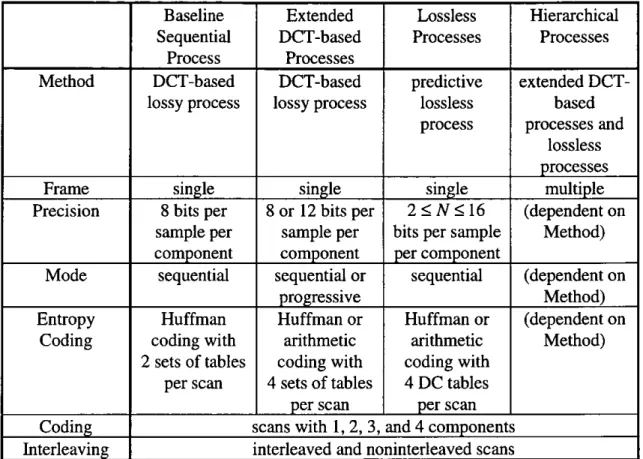
Chapter 3 JPEG Still Picture Compression Standard 45
3.1 Introduction 46
3.2 Background 46
3.3 Outline of the JPEG Standard 49
3.3.1 Image Components 49
3.3.2 Interleaving Image Components 50
3.3.3 An Example of Interleaved Image Components 51
3.3.4 Sample Precision 52
3.3.5 Modes of Operation 52
3.4 Baseline Sequential Process 54
3.4.1 DCT-based Coding 54
3.4.2 Level Shift prior to Forward Discrete Cosine Transform 56 3.4.3 8 x 8 Forward Discrete Cosine Transform 57
3.4.4 Quantization 58
3.4.5 DC Encoding and 2-D-to-l-D Zigzag Reordering 60
3.4.6 Huffman Encoding 62
3.4.7 Huffman Decoding 65
3.4.8 1-D-to-2-D Zigzag Reordering and DC Decoding 65
3.4.9 Dequantization 66
3.4.10 8 x 8 Inverse Discrete Cosine Transform 67 3.4.11 Level Shift after Inverse Discrete Cosine Transform 67
3.5 Remarks 67
3.6 Summary 69
Chapter 4 Adaptive Zigzag Reordering of Transform Coefficients 70
4.1 Introduction 71
4.2 Standard Zigzag Reordering 71
4.3 Adaptive Zigzag Reordering 75
4.3.1 Motivation for Adaptive Zigzag Reordering 75
4.3.2 Determination of Sub-blocks 75
4.3.3 Experimental Results 79
4.4 Versatile Zigzag-reordering Algorithm 83
4.4.1 Motivation for Versatile Zigzag-reordering Algorithm 83
4.4.2 The Sub-block 84
4.4.3 Parameters 85
4.4.4 The Truth Table 87
4.4.5 Boolean Expressions 91
4.4.6 The Binary Decision Tree 93
4.5 Hardware Implementation of Zigzag-reordering Algorithm 96 4.5.1 Motivation for Hardware Implementation of
Zigzag-reordering Algorithm 96
4.5.2 The GAL16V8 Device 96
4.5.3 The Tango-PLD Development Tool 98
4.5.4 The Moore State Machine for
Versatile Zigzag-reordering Algorithm 98
4.5.5 Implementation of Increments and Decrements 101
4.6 Coding of Sub-block Dimensions 103
4.6.1 Motivation for Coding of Sub-block Dimensions 103
4.6.2 The Sub-block Dimensions 103
4.6.3 Sub-block Dimensions and Scan-path Length 104 4.6.4 Entropy Coding of Sub-block Dimensions 110
Chapter 5 Artificial Neural Networks 113
5.1 Introduction 114
5.2 Introduction to Artificial Neural Networks 114
5.2.1 Biological Neural Networks 114
5.2.2 Foundations of Artificial Neural Networks 118 5.2.3 Properties of Artificial Neural Networks 119 5.2.4 Realization of Artificial Neural Networks 121 5.2.5 Applications of Artificial Neural Networks 122
5.3 Artificial Neuron 123
5.3.1 Structure of Artificial Neuron 123
5.3.2 Propagation Function 124
5.3.3 Activation Function 125
5.3.4 Output Function 126
5.3.5 Simplified Artificial Neuron 128
5.4 Feedforward Artificial Neural Networks 130
5.4.1 Structure of Feedforward Artificial Neural Networks 130
5.4.2 Forward Propagation 132
5.4.3 Learning 132
5.4.4 Hebb Rule 133
5.4.5 Delta Rule 134
5.4.6 Error-backpropagation Algorithm 135
5.4.7 Multilayer Feedforward Artificial Neural Networks 141 5.5 Artificial Neural Networks in Digital Image Compression 147
5.6 Summary 150
Chapter 6 Neural-network-based Block Classification 152
6.1 Introduction 153
6.2 Quantization of Transform Coefficients 153
6.3 Block Classification 154
6.3.1 Motivation for Block Classification 154 6.3.2 Structure of the Artificial Neural Network 156
6.3.3 Network Inputs 157
6.3.4 Network Outputs 159
6.3.5 Learning 159
6.4 Experimental Results 161
6.4.1 Implementation 161
6.4.2 Authentic Training Pairs 161
6.4.3 Learning 162
6.4.4 Classification 163
6.5 Summary 169
Chapter 7 Conclusions and Recommendations for Further Work 172
7.1 Introduction 173
7.2 Summary and Conclusions 173
7.3 Recommendations for Further Work 177
Appendices 205
A Landsat Image Size Worked Example A 1
B Huffman Tree Design Worked Example B 1
B.1 Introduction B 1
B.2 Design Procedure B 1
C JPEG Example Tables C 1
C.1 Introduction C 1
C.2 Quantization Tables C 1
C.3 Huffman Tables for 8-bit Precision C 2
D JPEG Baseline Sequential Process Worked Example D 1
D.1 Introduction D 1
D.2 Encoding Processing Steps D 1
D.3 Decoding Processing Steps D 4
D.4 Reconstruction Error D 8
E Images El
F Versatile Zigzag Reordering Algorithm Worked Example F 1
F. 1 Introduction F 1
F.2 Versatile Zigzag Reordering Algorithm F 1
G Hardware Implementation Source Files G 1
G. 1 Introduction G 1
G.2 Source File Stage A G 2
G.3 Source File Stage B G 6
G.4 Source File State Machine G 12
H Publications H 1
List of Tables
Table 2.1 Scales for Subjective Image Quality Assessment 40 Table 3.1 Component Parameters for Example of Three-component Image 51 Table 3.2 MCUs for Interleaved Scan of all Three Components for
Example of Three-component Image 52
Table 3.3 Essential Characteristics of the Distinct Coding Processes 54 Table 3.4 Magnitude Categories for Huffman Coding 63
Table 3.5 Additional Bits for Sign and Magnitude 63
Table 3.6 Coding Symbols for Huffman Coding of AC Coefficients 64 Table 4.1 Complete Truth Table for Changes in Row and Column Indices 88 Table 4.2 Reduced Truth Table for Changes in Row and Column Indices 90 Table 4.3 Truth Table for Construction of Binary Decision Tree 93
Table 4.4 Binary Increments 101
Table 4.5 Binary Decrements 102
Table 4.6 (1 of 3) Scan-path Lengths and Sub-block Dimensions 107 Table 4.6 (2 of 3) Scan-path Lengths and Sub-block Dimensions 108 Table 4.6 (3 of 3) Scan-path Lengths and Sub-block Dimensions 109 Table A. 1 Specification for Landsat-4 and -5 MSS and TM Images A 1
Table B. 1 Symbol Distribution of 8-level Image B 1
Table B.2 Sizes of 8-level Image B 4
Table C. 1 Example of Luminance Quantization Table C I Table C.2 Example of Chrominance Quantization Table C 1 Table C.3 Example of Luminance DC Difference Table C 2 Table C.4 Example of Chrominance DC Difference Table C 2
Table C.5 (1 of 4) Example of Luminance AC Table C 3
Table C.5 (2 of 4) Example of Luminance AC Table C 4
List of Figures
Figure 2.1 Generic Image-processing System 11
Figure 2.2 Typical Grey-level-to-luminance Transformation 12 Figure 2.3 General Model of Image-compression System 16
Figure 2.4 Transform-coding System 33
Figure 3.1 Data Units and Regions for Example of Three-component Image 52
Figure 3.2 DCT-based Coder Processing Steps 55
Figure 3.3 8 x 8 Forward DCT 58
Figure 3.4 Quantization 59
Figure 3.5 DC Coding 60
Figure 3.6 8 x 8 Zigzag Scan Path 61
Figure 3.7 DC Encoding and 2-D-to-1-D Zigzag Reordering 61 Figure 3.8 1-D-to-2-D Zigzag Reordering and DC Decoding 65
Figure 3.9 Dequantization 66
Figure 3.10 8 x 8 Inverse DCT 67
Figure 4.1 8 x 8 Block of Quantized DCT Coefficients 72
Figure 4.2 8 x 8 Zigzag Scan Path 72
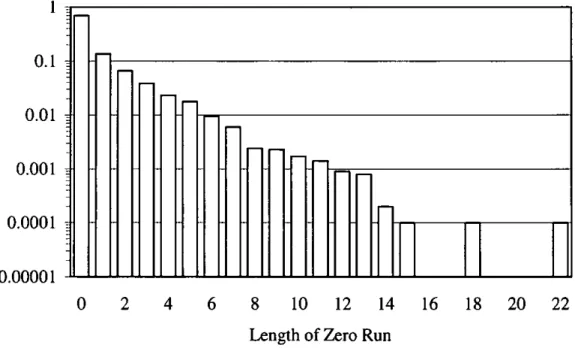
Figure 4.3 Probability Distribution of Runs of Zero Coefficients,
Standard Zigzag Reordering, Lena 512 x 512, q = 50 73 Figure 4.4 Decoded JPEG Image, Lena 512 x 512, q = 50 74 Figure 4.5 Example of 8 x 8 Block of Transform Coefficients 76
Figure 4.6 Example of Standard Zigzag Reordering 77
Figure 4.7 Example of Adaptive Zigzag Reordering 77
Figure 4.8 Probability Distribution of Runs of Zero Coefficients,
Adaptive Zigzag Reordering, Lena 512 x 512, q = 50 78 Figure 4.9 Probability Distribution of Sub-block Dimensions,
Lena512x512,q=50 79
Figure 4.10 Entropy of Runs of Zero Coefficients versus Quality Setting,
Lena 512x512 80
Figure 4.11 Entropy of Runs of Zero Coefficients versus Quality Setting,
Lena 256 x256 81
Figure 4.12 Entropy of Runs of Zero Coefficients versus Quality Setting,
Cameraman 256 x 256 81
Figure 4.13 Entropy of Runs of Zero Coefficients versus Quality Setting,
F-16 512x512 82
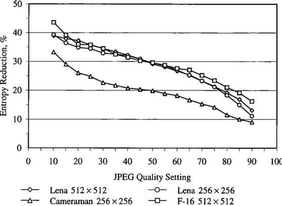
Figure 4.14 Entropy Reduction for Runs of Zero Coefficients versus
Quality Setting 83
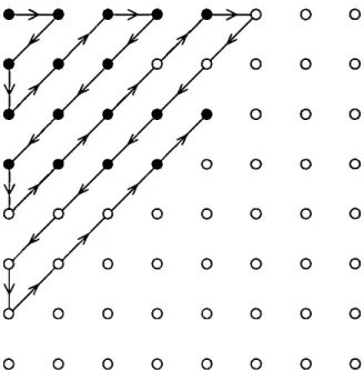
Figure 4.15 Directions of Movement 85
Figure 4.16 Decision Tree for Changes in Row and Column Indices 95 Figure 4.17 Functional Block Diagram of GAL16V8 Device 97 Figure 4.18 Block Diagram of Moore State Machine for
Versatile Zigzag-reordering Algorithm 99
Figure 4.19 Scan-path Length of 5 for (a) 5 xl, (b) 3 x 2, (c) 2 x 3,
and (d) lx 5 Sub-blocks 105
Figure 4.20 Scan-path Length of 14 for (a) 3 x 5, and (b) 4 x 5 Sub-blocks 106
Figure 5.1 Simplified Nerve Cell 115
Figure 5.2 Structure of an Artificial Neuron 123
Figure 5.3 Structure of a Simplified Artificial Neuron 128 Figure 5.4 Notation of a Simplified Artificial Neuron 129 Figure 5.5 Symbols for Functions of Artificial Neuron 129 Figure 5.6 Generic Feedforward Artificial Neural Networks 131 Figure 5.7 Structure of Error-backpropagation Algorithm 141
Figure 5.8 Single-layer Perceptron 142
Figure 5.9 Two-layer Perceptron 143
Figure 5.10 Two-layer Linear ANN 144
Figure 6.1 Quantization 154 Figure 6.2 ANN for Block Classification during Learning 156 Figure 6.3 ANN for Block Classification during Forward Propagation 157 Figure 6.4 Example of 8 x 8 Block of Transform Coefficients 158 Figure 6.5 Example of 8 x 8 Block of Amplitude Classifications 158 Figure 6.6 Example of 8 x 8 Block of Normalized Amplitude Classifications 159 Figure 6.7 MSE per Training Pair versus Epochs during Initial Learning Phase 162 Figure 6.8 MSE per Training Pair versus Epochs during Further Learning Phase 163 Figure 6.9 Entropy of Runs of Zero Coefficients versus
Peak-signal-to-noise Ratio, Lena 512 x 512 164 Figure 6.10 Entropy of Runs of Zero Coefficients versus
Peak-signal-to-noise Ratio, Lena 256 x 256 165 Figure 6.11 Entropy of Runs of Zero Coefficients versus
Peak-signal-to-noise Ratio, Cameraman 256 x 256 165 Figure 6.12 Entropy of Runs of Zero Coefficients versus
Peak-signal-to-noise Ratio, F-16 512 x 512 166 Figure 6.13 Decoded JPEG Image, Lena 512 x512, q = 65 167 Figure 6.14 Decoded Block-classified Image, Lena 512 x 512, q = 85 168 Figure 6.15 Entropy of Runs of Zero Coefficients versus
Peak-signal-to-noise Ratio, Different Weight Matrices
and Bias Vectors, Lena 512 x 512 169
Figure 7.1 Zigzag Scan Path for (a) 3 x 6, and (b) 6 x 3 Sub-blocks 178 Figure 7.2 New Zigzag Scan Path for (a) 3 x 6, and (b) 6 x 3 Sub-blocks 178
Figure B. 1 8-level Image B 1
Figure B.2 a) - e) Generation of a Huffman Tree for 8-level Image B 2 Figure B.2 f) - h) Generation of a Huffman Tree for 8-level Image B 3
Figure D. 1 8 x 8 Block of Source Samples D 1
FigureD.2 8 x 8 Block of Samples to FDCT D2
Figure D.4 8 x 8 Block of Quantized DCI Coefficients D 3
Figure D.5 1-D Vector of Reordered Values D 3
Figure D.6 Encoding of Intermediate Sequence of Symbols D 3
Figure D.7 Stream of Image Data D 4
Figure D.8 Decoding of Intermediate Sequence of Symbols D 5
Figure D.9 Reconstructed 1-D Vector D 5
Figure D. 10 Reconstructed 8 x 8 Block of Quantized DCI Coefficients D 6 Figure D. 11 8 x 8 Block of Dequantized DCI Coefficients D 6
Figure D. 12 8 x 8 Block of Samples from IDCT D 7
Figure D. 13 8 x 8 Block of Reconstructed Samples D 7
Figure D.14 8 x 8 Block of Error Values D8
Figure E. 1 Original Image, Lena 512 x 512 E 1
Figure E.2 Original Image, Cameraman 256 x 256 E 2
Figure E.3 Original Image, F-16 512 x512 E 3
Figure F. 1 Decision Iree for Changes in Row and Column Indices F 1 Figure F.2 Generation of Zigzag Scan Path for 3 x 2 Sub-block F 2
Acknowledgements
Firstly I would like to thank Martin R. Varley, my Director of Studies, for his consistent support and guidance through all stages of this research project, to which he has generously devoted much time and effort.
Next I would like to thank Trevor J. Terrell, my Second Supervisor, for the experienced guidance and direction he has given to the project.
I would also like to thank Phil Holifield, my Personal Tutor, for reading the first draft of the thesis and for many helpful discussions; and Isaac Y. K. Chan for the contributions to the publications.
I would like to thank the Department of Electrical and Electronic Engineering of the University of Central Lancashire for sponsoring my research studentship and providing the friendly learning environment.
Thanks are due to many members of staff for helping in various ways. I would like to single out vicariously late David Platt, Principal Technician, who is greatly missed. In addition, I would like to thank Playboy magazine for the kind permission to reproduce the images of Lena Sjoobloom; and Lattice Semiconductor for the kind permission to reproduce the functional block diagram of the GAL 16V8.
I wish to thank Bettina for her love and understanding that make me very grateful.
Finally I must thank my parents to whom I dedicate this thesis for their love, and their continuous encouragement and support. Danke!
Chapter 1
1.1
Introduction
In this chapter the research project is outlined, and brought in context to related disciplines of telecommunications and computing. Section 1.2 briefly highlights some of the important advances of these technologies. Section 1.3 describes the aims and objectives of the research project, and section 1.4 provides an overview of the thesis. Finally section 1.5 concludes the chapter with a brief summary.
1.2
Background
In 1837 Samuel Morse invented telegraphy, and seven years later he built the first telegraph line; between Washington and Baltimore, USA; which used Morse code. It was in 1851 that the first commercial transmissions using Morse code were established between England and France. In 1875 Alexander Graham Bell invented the telephone (A. Isaacs (ed.) 1997).
In 1920 the introduction of the Bartlane cable picture transmission system reduced the delivery time for newspaper pictures between London, England and New York, USA from one week to three hours using digital signals on transatlantic submarine cables (M. D. McFarlane 1972).
In 1948 William Shockley and co-workers invented the first transistors at Bell Telephone Co.
In 1962 the first active telecommunication satellite, US Telstar 1, was launched and positioned into relatively low elliptical orbit (A. Isaacs (ed.) 1997).
In the late 1970s microcomputers became widely available. These systems, typically having up to 16 KB random-access memory (RAM) and a tape drive, were used to manipulate text and numerical data, but offered limited graphical support. In the USA the Advanced Research Projects Agency Network (ARPANET) was commissioned as an experimental network designed to support military research. ARPANET later became the Internet.
In the 1980s personal computers, constantly growing more powerful, became available for office and home use. These systems, typically having up to 640 KB RAM, and floppy and hard disk drives, supported a large variety of applications, and offered from the late 1980s graphical user interfaces. However, because of enormous amounts of data involved, digital image processing was still limited to dedicated systems; see for example (G. Hall and T. J. Terrell 1987).
In the 1990s tremendous improvement of processing power, and increases of RAM and hard disk storage are transforming personal computers into powerful general-purpose systems suitable for processing digital image data. Additional networking capabilities of office and home computers allow the exchange of data among distant computers. The Internet, connecting a variety of different computers around the world and growing at great pace, changes the way individuals work and communicate; it symbolizes the information technology revolution.
With demand for transmission and storage of information rapidly growing, data compression in general and image compression in particular remain key technologies (N. Jayant et al. 1993); and, therefore, constitute important areas of research.
1.3 Aims and Objectives of the Project
The aims of the research described in this thesis were to investigate and develop appropriate neural-network models for digital image compression, and to develop the use of neural networks in hybrid schemes for image compression exploiting perceptually important features.
The specific objectives were:
• To review important existing image-compression techniques, • To review important existing neural-network models,
To develop new image-compression techniques or to improve existing ones, and To identify prospective directions for further research.
1.4 Organization of the Thesis
Chapter 2, entitled 'Digital Image Compression', places digital image compression in context to the human visual system and digital image processing, and focuses on some of the available techniques for lossless and lossy compression.
Chapter 3, entitled 'JPEG Still Picture Compression Standard', discusses the Joint Photographic Experts Group (JPEG) still picture compression standard in some detail as this compression standard has been adapted to a new hybrid compression scheme.
Chapter 4, entitled 'Adaptive Zigzag Reordering of Transform Coefficients', describes a new lossless transcoding scheme that adaptively reorders transform coefficients for improved coding efficiency, and includes experimental results to demonstrate the effectiveness of the scheme.
Chapter 5, entitled 'Artificial Neural Networks', introduces neural networks, and describes the backpropagation training algorithm in detail.
Chapter 6, entitled 'Neural-network-based Block Classification', describes a lossy scheme that uses an artificial neural network to classify blocks prior to adaptive zigzag reordering, and includes experimental results to demonstrate the effectiveness of the scheme.
Chapter 7, entitled 'Conclusions and Recommendations for Further Work', summarizes the contributions made by this thesis and offers recommendations for further research directions.
1.5 Summary
Since their invention telecommunications and computing have developed at great pace. The demand for exchanging information continues to grow, therefore data and image compression remain key technologies.
The main objective of the research described in this thesis has been to investigate the application of neural networks to digital image compression, particularly in hybrid schemes.
Chapter 2
2.1 Introduction
This chapter places digital image compression in context to the human visual system and digital image processing, and focuses on some of the available techniques for lossless and lossy compression.
Section 2.2 briefly summarizes the concept of digital image processing, introduces representations of digital images, and outlines a typical generic image-processing system.
Section 2.3 develops the necessity for digital image compression, distinguishes between lossless and lossy techniques, and summarizes the objectives of digital image compression. It introduces the three forms of data redundancy that can be exploited, and outlines a general image-compression model. The section also introduces entropy as a measure of the complexity of an information source.
Section 2.4 provides a very brief functional description of the human visual system, describes four properties as potentially being useful for digital-image-processing applications, and identifies two properties, spatial masking and local processing characteristic, as currently being most significant.
Section 2.5 describes a number of digital-image-compression techniques. It develops the concept of Huffman coding in detail, focuses also on run-length coding, quantization, and transform coding; and enumerates some other techniques.
Section 2.6 is concerned with image quality assessment based on subjective and objective measures. Finally section 2.7 concludes the chapter with a brief sununary.
2.2 Digital Image Processing
2.2.1 Motivation for Digital Image Processing
Digital image processing aims to gather, restore, enhance, relate, evaluate, and manipulate information contained in a digital image for many different purposes by means of computer technology; image samples are quantized to a fixed but sufficient number of information carrying units. Processing, storage, and transmission of digital representations of images offer many advantages over these operations performed on analogue representations: processing flexibility, easy or random access in storage, higher signal-to-noise ratio (SNR), possibility of error-free transmission, readiness for encryption and coding, and compatibility with other types of information as well as digital networks and computers, to name but a few. Image storage applications include medical imaging, image-based document management, and multimedia applications. Image transmission applications include broadcast television, remote sensing via satellites, aircraft, radar, sonar, teleconferencing, computer communications, and facsimile transmissions (A. K. Jain 1981).
2.2.2 Representation of Digital Images
An image is a 2-1) model representing a special and limited aspect of an observed scene. It contains only a very small part of the original information extracted from the electromagnetic energy spectrum; for example x-ray, ultraviolet, visible, and infrared bands; mechanical forces; for example pressure and torsion; or other physical measures using an appropriate sensor that produces an electrical signal proportional to the input signal.
Since the information is processed in digital computers, this signal must be digitized in location, i.e. image sampling, and amplitude, i.e. level quantization. Thus the continuous image is digitized on a grid of square or hexagonal sampling points by mapping the amplitudes to a linear or non-linear quantization function (M. Sonka et al.
1993, p. 27). The result is a raw image.
For common systems, spatial resolutions include 256 x 256, 512 x 512, 1024 x 1024, 360x576, and 720 x 576 picture elements (pixels); and 256-level quantization generates 8-bit integers ranging from 0, i.e. black, to 255, i.e. white.
Since data processing uses algorithms, and their implementations depend on the data representation, the data structure holding the digitized image data must be adequate. There is a variety of traditional and hierarchical image-data structures that can be categorized into different levels of abstraction.
A matrix A(L, M) of L rows by M columns of integer elements, each representing the brightness or another property of the corresponding pixel, holds the grid of pixels; and is the most common data structure for the direct representation of images. It can be defined as follows:
ra(l,!) a(1,2) . a(1,M)
1
a(2,l) a(2,2) a(2,M)
A(L,M)=I I (2.1)
a(1,m)
.
I
[a(L,1) a(L,2) . a(L,M)jThe matrix representation refers to the spatial domain; image data is accessible through the row and column indices of the associated pixels. Scanning or processing the matrix in left-to-right top-to-bottom order is purely a historical convention (R. J. Clarke 1995,
alternative. Many processing techniques benefit from this natural type of image-data
structure; for example digital image processing frequently uses arithmetic and logical
operations, filter operations often process overlapping sub-images, and compression
techniques often work on non-overlapping sub-images. Transformation of the image
into a different domain, for example using the fast Fourier transform (FF1') or the
discrete cosine transform (DCT) (N. Ahmed et al. 1974), and subsequent manipulation
in the transform domain is also used for processing and compression. Note that
intermediate representation with more quantization levels can minimize the propagation
of quantization errors (J. J. Rodriguez and C. C. Yang 1994).
While a single matrix can be interpreted as a grey-scale image, a matrix in a set of
matrices can contain information about one spectral band of a multispectral or colour
image. Alternatively, it can represent one instant in a time sequence of images. Since
most programming languages support matrices, i.e. 2-D arrays, the implementation of
this type of image-data structure is straightforward.
Other traditional image-data structures are chains, graphs, lists of object properties, and
relational databases. Hierarchical data structures comprising of pyramids and quadtrees
are means for more complex methods of image representation in computer vision
(M. Sonka et al. 1993, pp.
42-55).2.2.3
Digital-image-processing SystemA block diagram of a typical generic image-processing system is shown in figure 2.1.
Sensor and digitizer, i.e. analogue-to-digital converter, accomplish image acquisition.
Some sensors, for example charged-coupled device (CCD) cameras and scanners,
combine sensor and digitizer. Image data is manipulated by the processor; and stored
temporarily in internal memory, i.e. RAM, and permanently in mass storage, for example hard disk or tape. A keyboard accepts user input. A visual display unit (VDU), i.e. cathode-ray-tube (CRT) monitor, and other output devices, i.e. printer, are used to visualize the processed image data. The interface provides a link to other computers.
0
object
Figure 2.1 Generic image-processing System
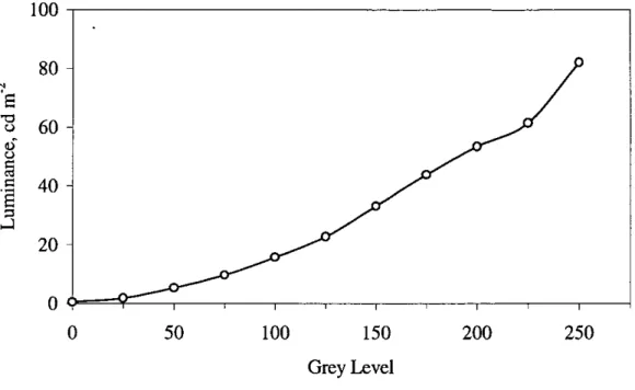
The display transforms the image data representing grey-level or colour values into luminance. Figure 2.2 depicts a typical transfer function (after S. A. Karunasekera and N. Kingsbury 1995).
However, as the function varies from display to display a faithful representation across computers is not achieved. The same problem applies to other input and output devices, and is addressed by device-independent colour management; see for example (Apple Computer 1995 and 1996).
100
CME
60
C) Uj40
20
[*1
0
50100
150
200
250Grey Level
Figure 2.2 Typical Grey-level-to-luminance Transformation
2.3
Introduction to Digital Image Compression2.3.1 Motivation for Digital Image Compression
Digital representations of images usually require enormous amounts of data; for
example one image taken by Landsat's multispectral scanner (MSS) consists of about
31 MB, and one image taken by Landsat's thematic mapper (TM) consists of about
263 MB; see appendix A for details. In addition the amount of image data being
collected, processed, stored, and transmitted increases rapidly because of higher
utilization, new applications, and higher standards. A recent survey (B. Foster 1996)
indicates for video microscopy a move toward higher spatial resolution, colour imaging,
and sending images across networks. For these reasons storing and transmitting data is,
and will remain, costly.
Processing of compressed images using efficient algorithms can also reduce the number
of operations required to implement an algorithm (A. K. Jain 1981); R. S. Ledley
(1993) proposed that the processing of medical images be carried out in the compressed
[Wi,
A large variety of compression techniques has evolved over the years. Implementations exist in software, hardware, and as mixed solutions. In general, if the digital image reconstructed from the compressed representation is numerically identical to the original digital image, the employed compression technique is lossless. Lossless compression techniques relate to machine vision, and to applications where gathered information is too valuable or legal reasons prohibit any loss of information (R. C. Gonzalez and R. E. Woods 1992, p. 343). If the reconstructed image only approximates the original image, the employed compression technique is lossy. While data compression must generally be fully reversible or lossless, lossy image-compression techniques sacrifice some information in order to achieve higher compression. Lossy techniques relate to applications for human perception, and should, therefore, be designed to minimize a perceptually meaningful measure of distortion, rather than more traditional and more tractable criteria such as the mean square difference between original and reconstructed image (N. Jayant et al. 1993).
2.3.2 Objectives of Digital Image Compression
The main objective of digital image compression is to develop efficient digital representations of images that minimize the number of information carrying units, the bit rate, in order to reduce storage and transmission requirements, and ultimately to reduce costs. The bit rate can be measured in bits element', bits pixeF' , or bits s
Secondary objectives include:
To minimize communication delay. The delay for encoding and decoding must match the requirements of an application. While, for example, real-time transmission demands short and same delay for encoding and decoding, the encoding delay for distribution via a storage medium is less important.
• To minimize complexity. The complexity is typically measured in terms of arithmetic capability, memory requirements, cost, and power consumption.
• To minimize the impact of errors on the reconstructed image.
• To support the exchange of compressed data among applications and across different computer systems as communication across networks grows in importance. This is addressed through standardization.
For lossy compression techniques an additional objective is to achieve the best image quality - however that might be defined - possible under given constraints.
The 'perfect' digital image-compression technique does not exist; the aim is, therefore, to minimize the bit rate in the digital representation of the image while maintaining required levels of image quality, complexity of implementation, and communication delay (N. Jayant et al. 1993). While, for example, a fixed bit rate in transmission results in varying quality, a fixed quality in storage causes a varying bit rate.
2.3.3 Data Redundancy
Three basic forms of data redundancy can be identified and exploited: coding redundancy, interpixel redundancy, and psychovisual redundancy. Digital image compression aims to remove redundancy and to reduce inelevancy by exploiting one or more types of data redundancy.
Coding redundancy is due to the fact that integer pixel values are usually represented through natural binary codes: every codeword consists of the same number of bits regardless of its statistical probability of occurring. Coding redundancy can be exploited by assigning shorter codewords to more probable pixel values and longer codewords to less probable ones.
Interpixel redundancy arises due to the fact that shapes and objects in an image extend usually over a region of pixels; pixel values are therefore fairly similar to their neighbours. Interpixel redundancy can be exploited by relating pixels to the adjacent pixels; for example the difference between adjacent pixels can be calculated in various ways and used to represent an image.
Psychovisual redundancy is due to the fact the human visual system does not respond with equal sensitivity to all visual information. Certain information has less relative importance than other information and can, therefore, be eliminated without significantly impairing the perceived image quality.
As the limits of compression exploiting coding and interpixel redundancies have been reached (M. Kunt et al. 1985), the move towards perceptual coding is natural.
2.3.4 Digital-image-compression Model
An image-compression system, depicted in figure 2.3, consists of encoder, channel representing a transmission path or a storage medium, and decoder; the human eye is generally the ultimate receiver at the end of the system. On a high functional level the encoder block processes the original representation and feeds the encoded data into the channel. After transmission over the channel, the encoded representation is fed to the decoder block that generates the reconstructed representation.
input .encoler decoder output
LJ
source channel channel channel source ______encoder encoder decoder decoder
origina reconstructed human
data data receiver
Figure 2.3 General Model of Image-compression System
Both the encoder and decoder consist of two sub-blocks. While, in an attempt to minimize the necessary bit rate for faithfully representing the input image, the source encoder removes data redundancies; the source decoder reverses the compression process. If an error-free system is required, it is the responsibility of the channel encoder-decoder pair to add redundancy to the encoded representation in order to recognize and correct any errors due to noise, distortion etc. introduced in the channel. However, the processes of source and channel coding can sometimes be integrated to increase efficiency of digital communication (N. Jayant et al. 1993). If the channel between encoder and decoder is noise free, the channel encoder and decoder can be omitted.
23.5 Entropy
The notion of coding is to find a new representation of an image that is smaller than the original representation of that image. Clearly, there is a lower bound that must depend on the image itself.
The histogram of an image represents the pixel distribution as a function of pixel value providing information on illumination conditions; contrast; range of values; and, maybe most importantly, probability distribution. If n, pixels have the k th of L possible pixel values Vk in an image consisting of n pixels, then the probability of occurrence of value Vft can be defined as
P(vk)= 5- k=[0,l,2,...,(L—l)] (2.2)
The discrete function relates the count of a pixel value n. to the total number of pixels n; probabilities range from zero, i.e. no occurrence, to one, i.e. exclusive occurrence. The sum of the probabilities is, of course, one:
P(v) = 1 (2.3)
Information theory models the generation of information as a probabilistic process; information content depends upon the probability of an event or symbol, i.e. pixel value in terms of image compression, occurring at each instance, i.e. pixel. Unlikely events, having low probability, carry more information than likely events, and vice versa. Ultimately, a certain event does not carry any information.
If the event E occurs with probability P(E), then the self-information of that event is defined as
1
1(E)=log =—log P(E) P(E)
The amount of self-information 1(E) attributed to event E is inversely related to its probability P(E); as P(E) approaches one, 1(E) converges towards zero. The base r of the logarithm in the above equation specifies r -ary units of information. However, the base 2 conveniently generating binary units, i.e. bits, can be defined as
1(E) = log 2 bits = —log 2 P(E) bits P(E)
1
(2.5) The entropy H, postulated by C. E. Shannon (1948a and b) as a measure of the complexity of an information source, defines the average amount of information conveyed per instance and can be defined as
H = —P(Ej )log r P(E)=
I
P(E1 )I(E) (2.6)where J denotes the total number of events.
As less certainty, and thus more information, is conveyed; the entropy H increases. If all events are equally probable, the entropy is at a maximum. The base r of the logarithm in the above equation specifies r -ary units of information. Again, the base 2 conveniently generating binary units, i.e. bits, can be defined as
(2.4)
Using the notation introduced in equation 2.2, the entropy of a digital image can be defined as
H = - P(vk) log 2 P(vk) bits (2.8)
Under the simplistic assumption that values of successive elements are statistically independent, i.e. no inter-element redundancy, the zero-order entropy H represents the lower bound: according to the noiseless coding theorem (C. E. Shannon 1948a and b), it is possible to encode information with entropy H bits elemenF' using
H + e bits elemen(t where E is an arbitrarily small positive quantity.
Entropy coding is a well-established lossless method for reducing the bit rate of digital images by exploiting the statistical redundancy in those images. It exploits the nonuniform probability distribution of pixel values, generally exhibited by images, by encoding the pixel values using variable-length codewords rather than equal-length codewords.
2.4 Human Visual System
2.4.1 Function of Human Visual System
It is generally the human visual system that perceives and judges images after processing or coding, therefore attempts should be made to incorporate knowledge about the properties of the human visual system to digital image compression and quality assessment. This section summarizes some important properties of the human visual system. Further reading includes a description of the eye (R. C. Gonzalez and R. E. Woods 1992, pp. 22-28) and the human visual system (M. Kunt et al. 1985), a
brief functional description (D. J. Sakrison 1977), and a description of interactions
among nerve cells in the retina (F. S. Werblin 1973).
The human visual system is a complex system in which the complexity of visual
perception increases as the image information propagates through the system. Image
information in the form of light intensity or luminance; that is a function of position,
time, and wavelength or frequency; enters the human visual system. Refraction by the
cornea, intraocular fluids, and lens focuses some of this information on the retina
forming a retinal intensity image as a function of retinal position, time, and wavelength.
Receptor cells at the back of the retina sense the intensities and, through a complex
network of interconnecting cells, encode the image into neural signals to be carried by
the optic nerve to the brain (D. J. Granrath 1981). Since optic-nerve fibres can only
accurately transport signals over a range much smaller than the range of image
information, the retina must compress the very large range of intensities presented by the
outside world into a narrower range that can be handled by the optic-nerve fibres.
The human visual system is an anisotropic system: from a given sensitivity at 00, i.e.
horizontality, its sensitivity decreases to a minimum at
45°and then increases again
reaching approximately the original level at 900 rotation. In addition, its sensitivity is
frequency dependent. Compared to the sensitivity at 00, the sensitivity at
45°to
frequencies of 10 and 30 cycles deg' is reduced by
15% and 30 % respectively
(C. F. Hall and B. L. Hall 1977). Spatial frequencies within a range of about one octave,
over a range of orientations of about 0
0
, are indistinguishable from each other
(W. B. Glenn 1993).
A comnon, but incomplete model of human vision incorporates a lowpass filter, a logarithmic nonlinearity, and a multichannel highpass filter; see (M. B. Sachs et al.
1971; C. F. Hall and E. L. Hall 1977; D. J. Sakrison 1977; and N. Jayant etal. 1993).
2.4.2 Relevant Properties of Human Visual System
It is the human eye that is generally the ultimate receiver of processed image data; see figure 2.3; therefore the properties of the human visual system should be considered, and suitable properties could be transferred to digital image compression. D. R. Fuhrmann et al. (1995) identified the following four properties as potentially being useful for digital-image-processing applications.
The human visual system responds to light in a nonlinear way. The smallest luminance difference that a human observer can detect when an object of a certain size is displayed at a certain background luminance level is defined as just-noticeable difference JND.
For a wide range of light intensities L the just-noticeable difference JND, or AL,
satisfies:
JND AL
= - = constant
L L (2.9)
This is known as Weber's law, and suggests a logarithmic relationship between the physical and 'perceived intensity of light, where the just-noticeable difference increases with increasing intensity. T. G. Stockham (1972), for example, proposed a visual model containing a logarithmic function and described its application to image enhancement. However, R. J. Clarke (1995, p. 8) reported that results of coding operations within a logarithmic/exponentiai domain had been inconclusive and argued that the conventional
display introduces a major nonlinearity in the processing chain that overrides the effects of the coding operations.
The human visual system performs spatial filtering. The optics of the eyeball have a lowpass characteristic. The lateral inhibition in the retina results in a highpass characteristic. The overall characteristic, that might be approximated by a bandpass characteristic, is centred somewhere between 4 and 8 cycles deg'; see (J. L. Mannos and D. J. Sakrison 1974; and R. J. Clarke 1985, p. 271, and 1995, pp. 7 and 75). Transform-based image-compression schemes offer a framework where the bit allocation of transform coefficients can be related to the spatial-frequency response, i.e. sensitivity, of the human visual system. Since only coefficients of the Fourier transform correspond directly to spatial frequency, the bit allocation must be modified for other transforms; H. Lohscheller (1984); N. B. Nill (1985); K. N. Ngan et al. (1989); and D. L. McLaren and D. T. Nguyen (1991) investigated the cosine transform. As the spatial frequency perceived by the eye depends on spatial resolution and viewing distance, the viewing conditions must be constrained. While a constant viewing distance of, for example, five times the image height (S. A. Karunasekera and N. Kingsbury 1995), and a fixed viewing position (D. R. Fuhrmann et al. 1995) can be obeyed for research purposes; these conditions cannot be assumed for practical applications in digital image compression. A. M. Lund (1993), for example, investigated viewing preferences, and found that the ratio of viewing distance to image height decreases as image size increases.
The human visual system performs spatial masking that is highly adaptive. This refers to the perceptibility of one signal in the presence of another in its time and frequency vicinity, and relates to the suppression of errors or distortion as a result of high image
activity or contrast. The aim of perceptual coding is to shape the error caused by lossy compression in a way so that the distortion is partially or fully masked by the signal, and therefore invisible to the human eye. In this context, it should be noted that high-frequency signals in visual information tend to have a short time or space support, while low-frequency signals tend to last longer (N. Jayant et al. 1993). Distortion masking, i.e. noise masking, has been incorporated in predictive and transform-coding techniques. The human visual system has a small visual angle of 1 to 3°. Complex images are viewed with a series of brief fixations and rapid eye movements (D. R. Fuhrmann et al. 1995). This leads to local rather than global processing characteristics: the human observer tends to concentrate on those areas in which degradation is most visible and to assess the overall quality accordingly; see for example (J. 0. Limb 1979; G. B. Legge and J. M. Foley 1980; and F. X. J. Lukas and Z. L. Budrikis 1982).
2.4.3 Significance of Human Visual System
As the properties of the human visual system govern the perception of visual information, digital image compression must take advantage of these properties in order to achieve lower bit rates by minimizing perceptually meaningful measures of distortion rather than more traditional criteria, such as the mean squared difference between the original and reconstructed image (N. Jayant et al. 1993). In digital image compression, coding bits can be allocated according to the importance of the information, in terms of the human visual system's sensitivity, that they convey. In quality assessment reliable numerical measures would allow efficient comparison of compression schemes, avoiding time consuming and expensive subjective tests under controlled conditions.
However, the human visual system and current digital-image-processing systems employ very different mechanisms.
While the human visual system responds to luminance, digital-image-processing systems manipulate grey-level or colour values that are transformed into luminance by the display. Since every display exhibits its own nonlinear transfer function, the perceived results vary from one digital-image-processing system to another.
While the human visual system responds to spatial frequency, digital-image-processing systems assume pixels of a certain size. The actual size of a pixel depends on the display, and the perceived spatial frequency is also a function of the viewing distance. For practical applications spatial masking and local processing characteristic are currently the most significant properties.
2.5 Digital-image-compression Techniques
2.5.1 Properties of Digital-image-compression Techniques
Techniques for digital image compression can be classified in various ways. The criteria of accuracy distinguishes between information-lossless and information-lossy techniques, as described in subsection 2.3.1. Compression can be carried out in spatial, frequency, transform, 'visual', or other domains. It can exploit coding, inter-element, and psychovisual redundancies individually or in combination. Algorithms can be designed to adapt their parameters affecting, for example, bit allocation or quantization levels to changes in image statistics.
Algorithms process elements, i.e. pixels for approaches in the spatial domain, individually; in rectangular or square blocks; or segments of elements having similar properties, i.e. shapes. Encoding of blocks offers potential for significantly better performance than encoding of each element individually, since the requirement to transmit at least some information for every element is relaxed. The disadvantage of arbitrarily dividing an image into rectangular or square blocks is that, as the bit rate is decreased, the block structure, that is easily perceived and irritating to the observer, appears in the reconstructed image (R. J. Clarke 1995, p. 76). Encoding based on shapes derived from actual image content rather than on blocks circumvents the disadvantage and may supersede block-based encoding.
Research work has produced a large variety of compression techniques. The following subsections describe those techniques, that are relevant to this thesis.
2.5.2 HufTman Coding
Huffman coding, a well-known entropy-coding technique, reduces coding redundancy by constructing a variable-length code that assigns the shortest possible codewords to the most probable events, or symbols, using integer numbers of code symbols, for example bits for binary codes. lluffman coding is lossless and codes elements individually, i.e. one at a time. Fluffman coding is optimal: it uses the variable-length code that achieves the minimum amount of redundancy possible when coding individual elements, i.e. for a particular set of symbols and their probabilities, no other integer code can be found that will give better coding performance than Huffman coding. It is a very popular technique used in many different schemes.
There are two basic restrictions imposed on the codewords:
• No two codewords consist of identical arrangements of code symbols.
• The code symbols are constructed in such a way that no additional indication is necessary to specify where a codeword begins and ends once the starting sequence of codewords is known.
For producing the minimum-redundancy variable-length code D. A. Huffman (1952) devised a method that builds up a tree by repetitively combining the least probable nodes, i.e. symbols and compound symbols, to a new node, i.e. compound symbol, with the summed probability until there is only one free node, i.e. the root node. Note that the probability of occurrence is proportional to the frequency of occurrence; see equation 2.2. Although r -ary trees can be built, binary trees are more popular. In non-adaptive schemes after the tree has been built and the code has been produced, encoding or decoding is simply accomplished by replacing original codewords with the Huffman codewords or vice versa. Storage and transmission of the code reduces efficiency.
A tree is a collection of nodes, that can contain information, and links, each connecting two nodes, that has certain properties. A path is a list of consecutive nodes that can be traversed via their links. The nodes directly succeeding a particular node are children of that node. In an ordered tree the order of the children is defined by some criteria. A node with at least one child is an internal node; a node without children is an external node. Internal nodes of a r -ary tree must have r children. The node directly preceding a particular node is the parent of that node, and the nodes also belonging to that parent are siblings. The one node without a parent is the root node. In a tree there exist exactly one path between the root node and every node, and exactly one path between any two nodes. The number of links from a node to the root node is the level, that can be used to
group nodes with the same distance from the root node. The internal path length is the sum of levels of all internal nodes. The external path length is the sum of levels of all external nodes. The path length is the sum of internal and external path length. In a binary tree every internal node has a left child and a right child, each of which can either be an internal or external node. Conventionally but arbitrarily, left children are identified by 0, and right children are identified by 1. Tracing the path from the root node to a particular external node generates a unique string of Os and is; see (R. Sedgewick 1992, chapters 4 and 22).
After generating the symbol distribution, the tree for a binary Huffman code can be built with the following steps (M. Nelson 1992, pp. 34-35); note that probability or frequency of occurrence is represented through a weight:
• Locate the two nodes with the lowest weights in the list of free nodes. Note that nodes with identical weights are equally suitable in term of coding gain, but may change the height, i.e. maximum level, of the tree if internal and external nodes have identical weights.
• Create a parent node for these two nodes, and assign a weight equal to the summed weights of the two child nodes to it. To generate an ordered tree, that is necessary for adaptive Huffman coding, ensure that the weight of the left child is less than or equal to the weight of the right child.
• Add the parent node to and remove the two child nodes from the list of free nodes. • Associate the left child node with 0, and the right child node with 1.
• Repeat above steps until only one free node is left. The free node is the root node of the tree.
Appendix B contains a worked example in which a lluffman tree is designed for an 8-level image of size 8 x 8.
The generation of the Huffman code can be equally described as a series of source reductions where the least probable source symbols are combined to form a new compound symbol with the summed probability that replaces the symbols from which it has been derived; see (R. C. Gonzalez and R. E. Woods 1992, pp. 343-345).
Huffman codes are instantaneous uniquely decodable block codes. They are called block codes, because each event is mapped to a codeword with a fixed sequence of code symbols, for example bits. They are instantaneous, because each codeword in a string of code symbols can be decoded without referencing succeeding events. They are uniquely decodable, because any string of code symbols can decoded in only one way without need for separation of the codewords (R. C. Gonzalez and R. E. Woods 1992, p. 345); see also (M. Nelson 1992, chapter 3; and R. J. Clarke 1995, appendix 1).
Non-adaptive Huffman schemes require two passes over the source symbols causing a delay: during the first pass the frequencies of occurrence of the events are collected, then the Huffman tree is constructed and stored or transmitted, and during the second pass the data is encoded. In adaptive Huffman schemes, the encoder and decoder start with identical initial trees, use the same algorithm to modify their trees and, therefore, stay synchronized. They require one pass, and are often more efficient than non-adaptive schemes; see (J. S. Vitter 1987).
Since codewords have to be an integer number of code symbols long, Huffman coding may have to assign either more or less code symbols to an event than theoretically necessary resulting in reduced efficiency; see equation 2.5. In general, Huffman coding
cannot reduce coding redundancy of data representing only two events, regardless of the probability distribution, since codewords require at least one code symbol.
2.5.3 Run-length Coding
Run-length coding exploits inter-element redundancy by representing a string of consecutive identical elements using a coding pair consisting of run length, that specifies the number of consecutive identical elements, and symbol, that specifies the value of the elements. Run-length coding is lossless. Although spatial-domain image data exhibits interpixel redundancy, strings of identical elements are rather short, especially in detailed natural images; however mn-length coding can be utilized for l-D and 2-D schemes in various ways. 2-D mn-length coding processes a scan line in context with transitions in the previous scan line.
Run-length coding of binary images, that have only black and white pixels, is employed in facsimile (fax) coding. Strings of Os and Is in each scan line, i.e. row, are coded from left to right. The value, 0 or 1, of the first string of each row is either specified, or the value of the first string is conventionally assumed to be 0. As the string values alternate between 0 and 1, an initial run length of zero indicates in the latter scheme that the row actually starts with a black string. Additional entropy coding, for example Huffman coding, can be used to reduce the coding redundancy of the run lengths. The run lengths of black and white can be coded separately using two entropy coders that are specifically tailored to the individual statistics; see (R. C. Gonzalez and R. E. Woods 1992, p. 354). Naturally, rn-bit images can be decomposed into m 1-bit bit planes that can be coded using mn-length coding for binary images. In order to reduce the effect of small grey-
representation of the image by an m -bit Gray code ensures that adjacent grey levels vary in only one bit plane; see (R. C. Gonzalez and R. B. Woods 1992, p. 350).
Assuming that in 8-bit images run lengths greater than 32, and pixel values greater than or equal to 224 would normally be rare; M. A. Sid-Ahmed (1995, p.400) described an algorithm that uses, dependent on the context, an 8-bit symbol with its three most significant bits set to 1 not as pixel value but as repeat count in the range [0,31] preceding the pixel value. Generally, run lengths greater than 1, and less than or equal to 32 are coded through pairs consisting of repeat count and pixel value. Single pixels with values greater than or equal to 224 are coded through pairs consisting of a repeat count that is equal to zero, i.e. 111000002, and the pixel value. However, single pixels with values less than 224 can simply be coded through the abbreviated 'pair' consisting only of the pixel value. Run lengths greater than 32 are coded by generating more than one coding pair.
The concept of run-length coding can also be applied to sparse matrices, that are usually represented through a list of nonzero elements and their indices. For example, the nonzero elements in each row or column are coded from left to right, or from top to bottom respectively. The distance between the preceding and current nonzero element, i.e. the number of zero elements in between, and the value of current non-zero element are combined to form a pair. The value of the first nonzero element is coded with reference to the beginning of the scan line. While each index can only appear once in every scan line, the distances can generally produce a distribution that has a lower entropy.
2.5.4 Quantization
Quantization exploits psychovisual redundancy by mapping a range of input values, for example pixel values or coefficients, to a limited number of output values, i.e. symbols. The range of input values, that can be continuous or discrete, is divided into a number of regions, each of which is represented by one output value. A set of output values is also referred to as a pulse-code-modulated (PCM) signal. As information is being lost during the many-to-one mapping, quantization is lossy and not fully reversible. However, during the inverse process, dequantization, each symbol is replaced with a value that represents the associated range of input values. The range of input values can be divided into regions in various ways.
Uniform quantization simply divides the range of input values into N equally sized regions separated by equally spaced decision levels d0 to dN, neither taking the probability distribution of the values into account nor trying to minimize the introduced distortion. The quantizer represents an input value greater than d1 and less than or equal to di,(d, , d, 1 ], by an output symbol of value i. The dequantizer generates a reconstructed value r, from a symbol i using:
= d1 + d1+1
2 (2.10)
Nonuniform quantization refers to a range division using unequally spaced decision levels. It is also known as optimal quantization, since this approach usually involves optimization of a statistical measure or psychovisual measure; see (A. N. Netravali 1977). The Lloyd-Max quantizer, independently developed by S. P. Lloyd (1982) and J. Max (1960), minimizes the mean-square quantization error by determining the best
values into account; see also (R. C. Gonzalez and R. E. Woods 1992, PP. 370-371; and M. A. Sid-Ahmed 1995, PP. 433-450).
Adaptive quantization adjusts the quantization levels based on the local probability distribution; see (A. N. Netravali and B. Prasada 1977). In a block-based spatial-domain scheme each block of image data is quantized using the quantizer, from a number of available quantizers, that introduces least distortion. The quantizers may be scaled versions of a Lloyd-Max quantizer for unit-variance Laplacian probability distribution, and the overhead associated with the quantizer selection is appended to each block; see (R. C. Gonzalez and R. E. Woods 1992, PP. 37 1-374).
2.5.5 Transform Coding
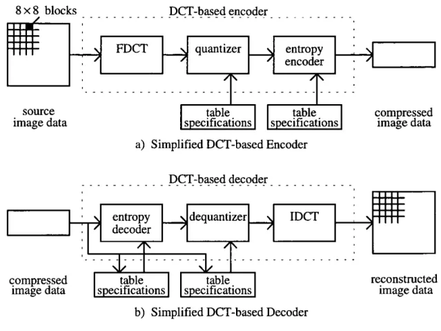
Transform coding describes a concept of a group of lossy digital-image-compression techniques, rather than one particular scheme, that has been incorporated into standards such as the JPEG still picture compression standard for lossy compression; see for example (0. K. Wallace 1992). The core of any transform-based coding system, that consists of a number of different coding stages, is a reversible, linear, 1-D or 2-D transform; that maps image data, i.e. a set of pixels, into a set of transform coefficients that has the same size. The purpose of this transform stage is to remove interpixel redundancy by converting statistically dependent pixel values into a set of 'less correlated' or 'more independent' coefficients. For most natural images a significant number of these coefficients have small magnitudes and can be coarsely quantized, or discarded entirely, with little image distortion (R. C. Gonzalez and R. E. Woods 1992, p. 374).
Figure 2.4 depicts a typical transform-coding system. During encoding the block selector splits the original image into blocks of pixels that are then processed by the forward transform to produce blocks of transform-domain coefficients. The quantizer, making transform-based coding lossy, maps each block into a set of symbols, i.e. quantized and scaled transform coefficients, which is then entropy-coded by the symbol encoder. The result is a continuous stream of encoded symbols. During decoding the decoder performs the inverse sequence of steps. The symbol decoder decodes the data stream and produces sets of symbols, each of which is mapped by the inverse quantizer into a block of quantized transform-domain coefficients, which is then processed by the inverse transform to produce a block of pixels. The block selector merges the blocks of pixels into the reconstructed image. While nonadaptive transform coding does not take local image content into account, adaptive transform coding enables one or more coding stages to respond to local image content; see for example (A. Habibi 1977).
input ---epçqdçr output
block forward symbol
selector I Itransforn encoder
original encoded
image data symbols
a) Encoder
input - --- decoder output
symbolinverse inverse block decoder quantizer ransfo selector
encoded --- reconstructed
symbols image data
b) Decoder
Figure 2.4 Transform-coding System
forward transfonn f(x,y) T(u,v) invent transfonn (2.11)
The spatial-domain representation f(x, y), i.e. a set of pixels, can be transformed into its transform-domain representation, i.e. a set of transform coefficients, and vice versa. The forward transform maps an L x M block of image data into an Lx M block of transform coefficients. Although 1-D transforms can be defined, 2-D transforms are a natural choice for digital image processing, that is concerned with 2-D image data. However, separable 2-D transforms are often implemented as two sets of 1-D transforms. 'Fast' implementations reduce the number of arithmetic operations.
A variety of transforms is available; for example FF1', DCT, Discrete sine transform (DST), Haar transform, Hadamard transform, Karhunen-Loève transform (KLT), Slant transform, and Walsh transform; see (R. C. Gonzalez and R. E. Woods 1992, chapter 3; and R. J. Clarke 1985). Selecting a transform for use in an image-compression scheme requires a compromise between transform efficiency and computational complexity to be made. The transform efficiency describes the transform's ability to decorrelate inter-element redundancy and to pack the energy that is spread across the image into as few transform coefficients as possible.
The 2-D FF1', a fast implementation of the 2-D discrete Fourier transform (DEl'), carries out a 2-D spectral analysis of the image data. Only Fourier transform coefficients correspond directly to measured spatial frequency; however, the transform efficiency is lower than that of other transforms.
The KLT transforms image data into a set of uncorrelated coefficients; and furthermore, for a given arbitrary number of retained transform coefficients, it minimizes the mean