Position control of electro-hydraulic actuator system using fuzzy logic controller optimized by particle swarm optimization

(1)

Edith Cowan University

Research Online

ECU Publications Post 2013

1-1-2013

Position control of electro-hydraulic actuator system using fuzzy

logic controller optimized by particle swarm optimization

Daniel M. Wonohadidjojo

Edith Cowan University, [email protected]

Ganesh Kothapalli

Edith Cowan University, [email protected]

Mohammed Hassan

Edith Cowan University

Follow this and additional works at: https://ro.ecu.edu.au/ecuworkspost2013

Part of the Civil and Environmental Engineering Commons

10.1007/s11633-013-0711-3

This is an Author's Accepted Manuscript of: Wonohadidjojo, D. M., Kothapalli, G. , & Hassan, M. (2013). Position control of electro-hydraulic actuator system using fuzzy logic controller optimized by particle swarm optimization. International Journal of Automation and Computing, 10(3), 181-193. The final publication is Available at

link.springer.com here

This Journal Article is posted at Research Online. https://ro.ecu.edu.au/ecuworkspost2013/21

(2)

Abstract:

Position control system of an Electro-Hydraulic Actuator System (EHAS) is investigated in this paper The EHAS is developed by taking into consideration the nonlinearities of the system: the friction and the internal leakage. A variable load that simulates a realistic load in robotic excavator is applied as the trajectory reference. A method of control strategy that is implemented by employing a Fuzzy Logic Controller (FLC) whose parameters are optimized using Particle Swarm Optimization (PSO) is proposed. The scaling factors of the fuzzy inference system are tuned to obtain the optimal values which yield the best system performance. The simulation results show that the FLC is able to track the trajectory reference perfectly for orifice opening. Orifice opening more than introduces chattering, where the FLC alone is not sufficient to overcome this. The PSO optimized FLC reduces the chattering significantly. This result suggests the implementation of the proposed method in position control of EHAS.

Keywords: Position control, Electro-Hydraulic Actuator, Fuzzy Logic Controller, Particle Swarm Optimization

1 Introduction

Position control applications in most equipments that are implemented using servo mechanism need robust control scheme and tracking accuracy. This requires good positioning and smooth response of the actuation system. Due to its capability, electro-hydraulic actuators have been used in this servo system for the last years. Its robustness and accuracy of position tracking contribute significantly in the applications and equipments such as robotics, mining, and aircraft.

The constraints appear in the applications of the hydraulic control system are the internal and external disturbances that yield the nonlinearities and uncertainties. Such characteristics emerge on the system and degrade its performance significantly. These disturbances have adverse impact on the robustness and accuracy of position tracking of the system. Such nonlinearities and uncertainties in the hydraulic actuation system are caused by the presence of friction and internal leakage of the system.

A number of studies have been conducted to minimise the impact of friction and internal leakage. An available nonlinear observer for Coulomb friction is modified to simultaneously estimate friction, velocity, and acceleration [1]. An observer-based friction compensating control strategy is developed for improved tracking performance of the manipulator. According to the nonlinearity and uncertainty of the excavator mechanism control system, in [2] a fuzzy plus PI controller which combines the advantages of fuzzy logic and conventional PI control is developed, a fuzzy rule based soft-switch method is adopted to achieve smooth switching.

In this paper, a method of position control of electro-hydraulic servosystem is proposed. This method introduces robustness to system nonlinearities and uncertainties. First, a fuzzy logic controller (FLC) is designed as the controller of the nonlinear model of electro-hydraulic system. The model takes into consideration the friction and internal leakage. Then the parameters of FLC is tuned by using the

Particle Swarm Optimization (PSO) algorithm. The parameters tuned are the scaling factors of the Fuzzy Inference System. To evaluate the performance and robustness of the proposed method, a computer simulation is used.

The structure of this paper is organized as follows: in section 2 we describe the mathematical models to develop the electro-hydraulic servosystem with the complete simulink model presented at the end of this section. The FLC design is explained in section 3. Then we explain the PSO in section 4. The testing and simulations of the position control of the electro-hydraulic actuator system are presented in section 5 followed by the results and discussion in section 6. We then conclude our study in section 7.

2 Electro-hydraulic actuator system

2.1 Hydraulic dynamics and force balance

model

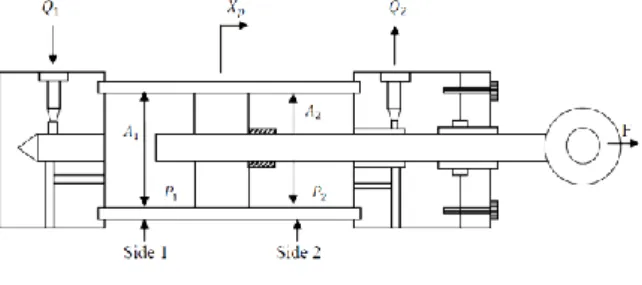
The electro-hydraulic actuator system modelled in this study consists of 2 main parts: the valve and the cylinder. The cylinder is modelled as a double acting single rod or single ended piston, with a single load attached at the end of the piston. The cylinder is depicted in Fig. 1 [3].

Fig. 1. Electro-hydraulic cylinder

Fig. 1 shows that Xp is the cylinder position, F denotes

Daniel Martomanggolo Wonohadidjojo

1

Ganesh Kothapalli

1

Mohammed Y. Hassan

2 1_{Edith Cowan University, WA6027, Australia}

2_{University of Technology, Baghdad, Iraq (Adjacent Academic, Edith Cowan University, WA6027, Australia)}

Position Control of Electro-Hydraulic Actuator using

(3)

Wonohadidjojo,D.M.et al. / International Journal of Automation and Computing

the applied load to the cylinder while Q1 and Q2 are the

fluid flow to and from the cylinder respectively. In Fig. 1, sides 1 and 2 are shown with the fluid pressure within side 1 is given by P1 and fluid pressure in side 2 is given by P2.

The pressurised area on side 1 and side 2 are shown in the Fig. 1 by A1 and A2 respectively. The cylinder will retract

or extend when a pressure difference between P1 and P2

occurs.

The dynamic of the system is expressed by:

𝑋̇p = Vp (1)

m.ap = Fa - Ff (2)

where Xp is the piston position, Vp is the piston velocity, ap

is the piston acceleration and m is the piston and load mass. There are two forces in (2) that influence the system: the hydraulic actuating force Fa and the friction force Ff which

are functions of nonlinearities that will significantly influence the system. The parameters that affecting Fa are

the control input voltage, environment load, cylinder pressure, friction force and leakage. Hence, it can be represented by:

Fa = Ap.Pl (3)

Therefore, the force balance equation of the cylinder is represented by:

𝑚𝑎𝑝= 𝐴𝑝𝑃𝑙− 𝐹𝑓 (4)

where Ap is the cross section of the hydraulic cylinder and

Pl is the cylinder differential pressure, which can be written

as:

𝑃𝑙= 𝑃1− 𝑃2 (5)

The differential equation in (4) governs the dynamics of the system.

As discussed in [4], by defining the load pressure Pl to

be the pressure across the actuator piston, the derivative of the load pressure is given by the total load flow through the actuator divided by the fluid capacitance:

𝑉𝑡

𝛽𝑒𝑃̇𝑙 = 𝑄𝑙− 𝐶𝑡𝑃𝑙− 𝐴𝑃𝑉𝑃 (6)

where Vt is the total actuator volume of both cylinder sides,

𝛽e is the bulk modulus of hydraulic oil, Ct is the total

leakage coefficient, and Ql is the load flow. By using (6),

the flow equation of the servo valve is given in (7). It expresses the relationship between spool valve displacement Xv and the load flow Ql.

𝑄𝑙= 𝐶𝑑𝑊𝑋𝑣√𝑃𝑠−𝑠𝑔𝑛(𝑋_𝜌 𝑉)𝑃𝑙 (7)

where Cd is discharge coefficient, W is the spool valve area

gradient and 𝜌 is the oil density. By substituting (7) into (6) one can find the hydraulics dynamics of the cylinder pressure in (8).

𝑃̇𝑙=4𝛽_𝑉𝑒

𝑡 [−𝐴𝑃𝑉𝑝− 𝐶𝑡𝑃𝑙+ 𝐶𝑑𝑊𝑋𝑣√

𝑃𝑆−𝑠𝑔𝑛(𝑋𝑣)𝑃𝑙

𝜌 ] (8)

The spool displacement of the servo valve Xv is controlled

by the control signal generated by the FLC U. The corresponding relation can be simplified as:

𝑋̇𝑣=_𝜏1

𝑣(−𝑋𝑣+ 𝑘𝑣𝑢) (9)

The servo valve input can also be expressed as a second

order lag: 𝑢 =_𝑘1 𝑣( 1 𝜔𝑣2𝑥̈𝑣+ 2𝐷𝑅𝑣 𝜔𝑣 𝑥̇𝑣+ 𝑥𝑣) (10)

where kv is the servo valve gain, 𝜏v is time constant, 𝜔v is

the natural frequency and 𝐷𝑅𝑣 is the damping ratio of servo

valve. Based on equation (1) to (10), if the state variables are determined as

𝑥 = [𝑥1, 𝑥2, 𝑥3]𝑇≡ [𝑥𝑝, 𝑣𝑝, 𝑎𝑝] 𝑇

(11) then a third order of state equations model for a servo hydraulic actuator system can be obtained by neglecting the valve dynamic (9) and replace it by (12).

𝑋𝑣= 𝑘𝑣𝑈 (12)

Then the following equations can be obtained:

𝑥̇1= 𝑥2 (13)

𝑥̇2= 𝑥3 (14)

𝑥̇3= 𝑎̇𝑝=_𝑚1(𝐴𝑝𝑝̇𝑙− 𝐹̇𝑓) (15)

2.2 Friction model

Friction is an important aspect of many control systems both for high quality servo mechanisms and simple pneumatic and hydraulic systems. Friction can lead to tracking errors, limit cycles, and undesired stick-slip motion [5]. Friction is the tangential reaction force between two surfaces in contact. Physically these reaction forces are the results of many different mechanisms, which depend on contact geometry and topology, properties of the bulk and surface materials of the bodies, displacement and relative velocity of the bodies and presence of lubrication [6]. The commonly used model for friction is usually depicted by the discontinuous static mapping between velocity and friction force. This needs to consider the Coulomb and viscous friction that depends on the velocity sign. The static model, however, does not take into consideration the dynamics behaviour of the friction force such as stick-slip motion, re-sliding displacement and friction lag. These characteristics are properties of friction in nature, therefore, friction does not have instantaneous response to the velocity change. In order to model the static and dynamic behaviour of friction force, LuGre model [6] is used in the design of friction in this study. It accommodates both static and dynamic characteristics of the friction force. Fig. 2 shows the characteristic of friction – velocity of this model. The friction characteristics are generated during two cycle of oscillation. The oscillation results in a narrow hysteretic effects around the zero relative velocity in the graph (presliding motion area)[7].

Fig. 2. Characteristic of friction force – velocity [4] LuGre model is expressed by:

(4)

𝐹𝑓= 𝜎0𝑧 + 𝜎1𝑧̇ + 𝜎2𝑣𝑝 (16)

𝑧̇ = 𝑣𝑝−_𝑔(𝑣|𝑣𝑝|

𝑝)𝑧 (17)

where z is the average deflections of the bristle between each pair of the contact surface that is described by the friction internal state andvpis the relative velocity between

two surfaces 𝝈0, 𝝈1, and 𝝈2are the stiffness of the bristle

between two contact surfaces, bristles damping coefficient, and viscous friction coefficient respectively. The nonlinear property of friction is described by g(vp) in (18), which can

be parameterized to characterize the Stribeck effect.

𝑔(𝑣𝑝) =_𝜎1 0[𝐹𝑐+ (𝐹𝑠− 𝐹𝑐)𝑒 −(𝑣𝑝 𝑣𝑠) 2 ] (18) 𝐹𝑐, 𝐹𝑠 and 𝑣𝑠 are the Coulomb friction, viscous friction and

stribeck velocity, respectively. With this description, the model is characterised by four static parameters and two dynamic parameters, stiffness coefficient and damping coefficient.

2.3 Internal leakage model

At small servo valve spool displacements, leakage flow between the valve spool and body dominates the orifice flow through the valve [8]. In precision positioning applications, where the servo valve operates within the null region, this flow, if ignored, may severely degrade the performance of a conventional servo hydraulic design. In this study, an accurate model of leakage flow [8] is used. It includes both leakage flow and orifice flow, and makes smooth transition between them would likely improve precision of the servo hydraulic system design and performance. The model used is a nonlinear servo valve model that accurately captures the servo valve leakage behaviour over the whole ranges of spool movement. The leakage behaviour is modelled as turbulent flow with a flow area inversely proportional to the overlap between the spool lands and the servo valve orifices.

A servo valve configuration depicted in Fig. 3, consists of two control ports with variable orifices regulate the flow rates. The flow rates through the control ports of the servo valve are expressed in (19) and the flow rate at the supply and return ports are represented in (20).

Fig. 3. Hydraulic servo valve configuration

𝑄1= 𝑄1𝑆− 𝑄1𝑅 and 𝑄2= 𝑄2𝑅− 𝑄2𝑆 (19)

𝑄𝑆= 𝑄1𝑆+ 𝑄2𝑆 and 𝑄𝑅= 𝑄1𝑅+ 𝑄2𝑅 (20)

The flow rate at the supply side and return side of control port 1 are given by:

𝑄1𝑆= 𝐾1𝑆√(𝑃𝑆− 𝑃1)(𝑋0+ 𝑋𝑣) (𝑋𝑣≤ 0) (21)

𝑄1𝑅= 𝐾1𝑅√(𝑃1− 𝑃𝑅)𝑋02(𝑋0+ 𝑘1𝑅𝑋𝑣)−1(𝑋𝑉≥ 0) (22)

where 𝑋0 is the leakage flow rate at null (𝑋𝑣 = 0). 𝑋0 is

equivalent to a spool displacement that would result in the same amount of flow in a nonleaking servovalve as the leakage flow rate in a leaking servovalve with a centered spool. Since the leakage resistance increases at larger valve openings, the leakage flow rate is inversely proportional to spool displacement [8].

The relations for orifice and leakage flow at the servovalve ports form the basis of the servo valve flow model. For negative spool displacement, the flow relations are interchanged since now the supply side forms the leakage path and the return side flow is an orifice flow. Applying similar reasoning to each orifice, we obtain the flow relations for control port 1 [8]:

𝑄1𝑆= 𝐾1𝑆(𝑃𝑆− 𝑃1)1/2{(𝑋_𝑋0+ 𝑋𝑉), (𝑋𝑉≥ 0) 02(𝑋0− 𝑘1𝑆𝑋𝑉)−1, (𝑋𝑉< 0) (23) 𝑄1𝑅= 𝐾1𝑅(𝑃1− 𝑃𝑅)1/2{𝑋0 2_(𝑋 0+ 𝑘1𝑅𝑋𝑉)−1, (𝑋𝑉≥ 0) 𝑋0− 𝑋𝑉, (𝑋𝑉< 0) (24)

For control port 2, the flow relations are:

𝑄2𝑆= 𝐾2𝑆(𝑃𝑆− 𝑃2)1/2{𝑋0 2_(𝑋 0+ 𝑘2𝑆𝑋𝑉)−1, (𝑋𝑉≥ 0) 𝑋₀− 𝑋_𝑉, (𝑋_𝑉< 0) (25) 𝑄2𝑅= 𝐾2𝑅(𝑃2− 𝑃𝑅)1/2{ (𝑋0+ 𝑋𝑉), (𝑋𝑉≥ 0) 𝑋02(𝑋0− 𝑘2𝑅𝑋𝑉)−1, (𝑋𝑉< 0) (26)

The total supply flow 𝑄𝑆 represents the internal leakage

flow since the control ports are blocked for an internal leakage test [9]. The internal leakage flow can be expressed by: 𝑄𝑆= 2𝐾𝑓(𝑃𝑆− 𝑃𝑅) 1 2(𝑋₀+ |𝑋_𝑣|)(1 + 𝑓(𝑋))−1/2 (27) where 𝑓(𝑋𝑣) = [1 +|𝑋_𝑋𝑣| 0] 2 [1 + 𝑘𝑓|𝑋_𝑋𝑣| 0] 2 (28) For any type of servo valve, available manufacturer data (Qmax and Imax) can be used to determine the servo valve leakage parameters such as 𝐾𝑓, 𝑘𝑓 and 𝑋0 [8].

Having discussed the electro-hydraulic actuator model, the LuGre friction model and the internal leakage model,

(5)

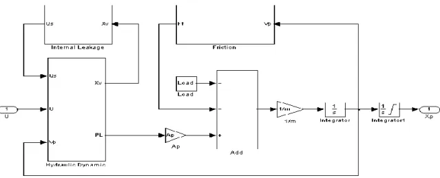
Fig. 4.The simulink block diagram of electro-hydraulic actuator system with friction and internal leakage we then integrate them into an integrated model. The

friction model is integrated by supplying the output of equations (16) to (18) into the model. The internal leakage model in (23) to (27) are integrated into (6) and (7) to determine the total supply flow into side 1 of the cylinder. The simulink block diagram of electro-hydraulic servosystem with friction and internal leakage modelled from equations (1) to (28) is shown in Fig. 4. The next section will discuss the FLC used to control the position of EHS model that contains friction and internal leakage.

3 Fuzzy Logic Controller

3.1 Fuzzy Inference System

The control strategy of the EHS needs to be able to overcome the nonlinearities and uncertainties emerge from the system. A controller with robust tracking performance is obviously significant. A fuzzy logic controller is designed to fulfil the need for such controller.

Fuzzy control provides a formal methodology for representing, manipulating, and implementing a human’s heuristic knowledge about how to control a system [10]. The fuzzy logic controller block diagram is given in Fig. 5. The fuzzy controller has four main components: (1) The “rule-base” holds the knowledge, in the form of a set of rules, of how best to control the system. (2) The inference mechanism evaluates which control rules are relevant at the current time and then decides what the input to the plant should be. (3) The fuzzification interface simply modifies the inputs so that they can be interpreted and compared to the rules in the rule-base, and (4) the defuzzification interface converts the conclusions reached by the inference mechanism into the inputs to the plant [10].

3.2 Universe of discourse

The FLC is designed as a Proportional Integral (PI) fuzzy logic controller where the equation giving a conventional PI-controller is

u(t) = Kp.e(t) + Ki.∫ 𝑒(𝑡)𝑑𝑡 (29) where Kpand Kiare the proportional and the integral gain coefficients respectively. A block diagram for a PI like

fuzzy logic control system is depicted in Fig. 6 [11].

Fig. 5. The fuzzy logic controller block diagram.

Based on Fig. 6, it is clear that the FLC has two input variables: error and change of error. The output variable of the controller is the control signal to control the plant. Thus the FLC is a two inputs and one output system. Fig. 7 shows the block diagram of the FLC controlled integrated EHAS in a closed-loop control system. The system output is denoted by y(t), its inputs are denoted by u(t), and the reference input to the fuzzy logic controller is denoted by

r(t).

3.3 Membership functions

The universe of discourse in the Fuzzy membership function designed for the error, change of error and the output is normalised with -1 to 1 span. The linguistic values of the error and change of error are designed with 7 linguistic terms for each input: Negative Big (NB), Negative Medium (NM), Negative Small (NS), Zero (Z), Positive Small (PS), Positive Medium (PM), and Positive Big (PB). The same linguistic terms are used for the output. Each linguistic value is assigned a triangular membership function. The membership functions of inputs and output are shown in Fig. 8, Fig. 9 and Fig. 10.

Inference Mechanism Knowledge Base

Fuzzi

fi

cat

ion

D

ef

uzzi

fi

czt

ion

(6)

Set point Error Ki Output + Ku - + Kp - Change of error

Fig. 6. Block diagram of a PI fuzzy control system

Reference u(t) y(t) Input +

r(t) -

Fig. 7. Fuzzy logic controlled integrated hydraulic model in a closed-loop control system

Fig. 8. Membership functions of Error as input

Fig. 9. Membership functions of Change of Error as input

Fig. 10. Membership functions of control signal as output

3.4 Rules

Using the 7 linguistic values for each input and 7 values for the output, in this study the FLC is designed with 49 rules. These rules were selected using trial and error method. The rule base is presented in Table 1.

Table 1. Rules Base of the FLC

3.5 FLC Tuning

After the design of FLC completes, then it is connected with the plant to be controlled which is the integrated model of the electro-hydraulic system. This forms a closed loop system with the FLC as the controller and output of the plant is observed as the feedback to be compared with the reference input. The simulink block diagram of closed loop system is depicted in Fig. 11.

The rest of the process will be the simulation of the whole system and tuning of the FLC. The objective is to obtain the best system performance. This can be accomplished by tuning the values of scaling factors: Kp, Ki and Ku that resulting in the minimum oscillation, overshoot and error.

Fig. 11. Simulink block of the FLC controlled integrated EHAS in closed loop system

Tuning of FLC parameters using trial and error method does not always give the optimum results. In addition, it is a time consuming process. Therefore, an intelligent optimization technique to optimize the FLC parameters is obviously neccessary. The next section discusses the Particle Swarm Optimization.

-1 -0.5 0 0.5 1 0 0.2 0.4 0.6 0.8 1 Output D eg re e of m em be rsh ip NB NM NS Z PS PM PB

PI-like

FLC

Delay

∆

t

∫

P

l

a

n

t

PI-like FLC Integrated Hydraulic Model

(7)

4 Particle Swarm Optimization

In 1995, Kennedy and Eberhart introduced Particle Swarm Optimization (PSO) as an evolutionary algorithm. Particle Swarm Optimization (PSO) is inspired by swarming behaviours observed in flocks of birds, schools of fish, or swarms of bees. PSO is a population-based optimization tool, which could be implemented and applied to solve various function optimization problems, or the problems that can be transformed to function optimization problems. This method was developed through simulation of a simplified social system, and has been found to be robust in solving continuous nonlinear optimization problems [12,13].

In PSO, each particle is attracted toward the position of current global best 𝑔∗_{and its own best location}_𝑥

𝑖∗ in

history, while the same time it has tendency to move randomly. When a particle finds a location that is better than any previously found locations, then it updates it as the new current best for particle i. There is a current best for all n particles at any time t during iterations. The aim is to find the global best among all the current best solutions until the objective no longer improves or after a certain number of iterations. The essential steps of the PSO can be summarised as the pseudo code shown in Fig. 12.

Particle Swarm Optimization

Objective function 𝑓(𝑥), 𝑥 = (𝑥1, … , 𝑥𝑝) 𝑇

Initialise locations 𝑥𝑖 and velocity 𝑣𝑖 of n particles Find 𝑔∗_{from min}_{𝑓(𝑥

1), … , 𝑓(𝑥𝑛)} (at t=0) While (criterion)

T=t+1 (pseudo time or iteration counter) for loop over all n particles and all d dimensions Generate new velocity 𝑣𝑖𝑡+1using equation (30) Calculate new locations 𝑥𝑖𝑡+1= 𝑥𝑖𝑡+ 𝑣𝑖𝑡+1 Evaluate objective functions at new locations 𝑥𝑖𝑡+1 Find the current best for each particle 𝑥𝑖∗

End for

Find the current global best 𝑔∗ End while

Output the final results 𝑥𝑖∗ and 𝑔∗

Fig. 12. Pseudo code of Particle Swarm Optimization [14] When 𝑥𝑖 and 𝑣𝑖 are the position vector and velocity for

particle i respectively, then the new vector is determined by (30).

𝑣𝑖𝑡+1= 𝑣𝑖𝑡+ 𝛼𝜖1∙ [𝑔∗− 𝑥𝑖𝑡+1] + 𝛽𝜖2∙ [𝑥𝑖− 𝑥𝑖𝑡] (30)

where 𝜖1 and 𝜖2 are two random vectors, and each entry

taking the values between 0 and 1. The parameters 𝛼 and 𝛽 are the learning parameters or acceleration constants, which can typically be taken as 2 [14].

4.1. Accelerated PSO

The accelerated PSO based on [14 ] is used in this study. The standard PSO uses both the current global best 𝑔∗_and

the individual best 𝑥𝑖∗. The reason of using the individual

best is primarily to increase the diversity in the quality solutions, however, this diversity can be simulated using some randomness. Subsequently, there is no compelling reason for using the individual best, unless the optimization problem of interest is highly nonlinear and multimodal

[14].

As discussed in [14], a simplified version which could accelerate the convergence of the algorithm is to use the global best only. Thus, in the accelerated PSO, the velocity vector is generated by a simpler formula

𝑣𝑖𝑡+1= 𝑣𝑖𝑡+ 𝛼 (𝜖 − 1 2) + 𝛽(𝑔

∗_{− 𝑥}

𝑖𝑡) (31)

where 𝜖 is a random variable with values from 0 to 1. We can also use a standard normal distribution 𝛼𝜖𝑛 where 𝜖𝑛

is drawn from N(0,1) to replace the second term. The update of the position is simply

𝑥𝑖𝑡+1= 𝑥𝑖𝑡+ 𝑣𝑖𝑡+1 (32)

In order to increase the convergence even further, the update of the location in a single step can also be written: 𝑥𝑖𝑡+1= (1 − 𝛽)𝑥𝑖𝑡+ 𝛽𝑔∗+ 𝛼𝜖𝑛 (33)

This simpler version will give the same order of convergence. The typical values for this accelerated PSO are 𝛼 ≈ 0.1~0.7, though 𝛼 ≈ 0.2 and 𝛽 ≈ 0.5 can be taken as the initial values for most unimodal objective functions. It is worth pointing out that the parameters 𝛼 and 𝛽 should in general be related to the scales of the independent variables 𝑥𝑖 and the search domain.

A further improvement to the accelerated PSO used in [14] is to reduce the randomness as iterations proceed. This means that we can use a monotonically decreasing function such as

𝛼 = 𝛼0𝑒−𝛾𝑡 (34)

or

𝛼 = 𝛼0𝛾𝑡, 0 < 𝛾 < 1) (35)

where 𝛼0≈ 0.5~1 is the initial value of the randomness

parameter. Here t is the number of iterations or time steps. 0 < 𝛾 < 1 is a control parameter, where 𝑡 ∈ [0,10]. Obviously, these parameters are fine-tuned to suit the current optimization problem.

4.2 PSO Implementation

The parameters used in the PSO are: number of particles: 25, dimension of the problem: 3, number of maximum iteration: 500, speed of convergence (𝛽 = acceleration coefficient determining the scale of the forces in the direction of 𝑝𝑖): 0.5, randomness amplitude of

roaming particles (𝛼 = acceleration coefficient determining the scale of the forces in the direction of 𝑔𝑖): 0.2, and

𝛾 = 0.95.

The PSO is employed to optimize the FLC parameters (scaling factors): KI, KP, KU. These factors are optimized at the same time. The functions of these parameters in the FLC are shown in (36).

∆𝑢(𝑡) = 𝐾 . 𝑒(𝑡) + 𝐾𝑝. ∆𝑒(𝑡) (36)

The fitness function of the problem is the Integral of Time multiplied by Absolute Errors (ITAE):

𝐼𝐼𝑇𝐴𝐸= ∫ 𝑡|𝑒(𝑡)|𝑑𝑡₀𝑇 (37)

The fitness function considered is based on the error criterion. The performance of a controller is evaluated in terms of error criterion. Fig. 13 shows the closed loop system of the integrated EHAS controlled by PSO optimized FLC.

(8)

Fig. 13. PSO optimized FLC controlled integrated EHAS in a closed loop system.

5 Tests and simulations

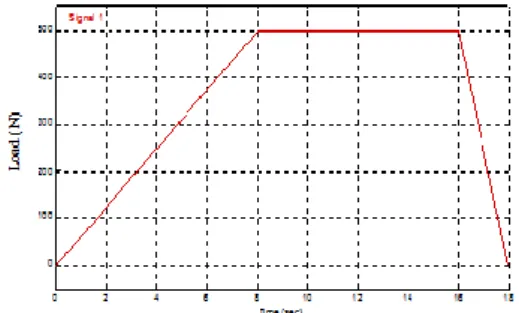
The simulation tests were conducted to evaluate the performance of the closed loop system under the prescribed environments. The system was tested to handle variable load with 500N maximum value of the load and friction parameters specified in Appendix. The variable load is depicted in Fig. 14.

First the test was undertaken using several orifice openings. The tests were undertaken from small opening to bigger orifice openings. These were applied in the system while the results were observed to evaluate the response and performance of the system.

Fig. 14. Variable Load of the closed loop system

6 Results and Discussion

First, a 8e-5 orifice opening was applied in the system, and the result is shown in Fig. 15.

Fig. 15. Response of the FLC controlled system with 8e-5 orifice opening

Fig. 15 shows the result of simulation with trajectory reference, variable load, and friction parameters described in section 5. The system is able to track the trajectory

reference accurately, and there is no overshoot and steady state error in the system output.

Using the same trajectory reference, variable load, and friction parameters, then bigger orifice openings were applied in the system. At 229e-5 opening, a chattering was observed for the first time. Further test was conducted to observe and evaluate a more visible chattering, a 235e-5 opening was applied in the system. The system response is depicted in Fig. 16.

Fig. 16. Response of FLC controlled system with 235e-5 orifice opening

It can be seen from the result, that the 235e-5 orifice opening introduces deflection and chattering in the system output. The deflection started from 8s when the variable load reaches its maximum value until the chattering occurs from 14s to 18s of the simulation time. After that, the system output is able to track the trajectory reference with no error. This indicates that the FLC is not able to handle anymore the nonlinearities in the system introduced by the orifice opening. The FLC cannot handle the orifice openings starting from 229e-5.

Then the next test was undertaken by employing PSO to optimise the FLC parameters, by using the same trajectory reference, variable load, friction parameters, and with 235e-5 orifice opening. The result is shown in Fig. 17.

Fig. 17. Response of the PSO optimized FLC controlled system with 235e-5 orifice opening

It is shown in Fig. 17 that the deflection in the system output still occurs from 8s, but the chattering is now reduced only from 14s to approximately 15.2s. This means that the PSO is able to reduce the chattering in the system.

(9)

The result shows the effectiveness of the PSO to optimize the FLC parameters in order to reduce the chattering introduced by the nonlinearities in the EHAS. The simulation results indicate that PSO has been successfully implemented to optimize the FLC parameters in the EHAS.

7 Conclusions

The position control of electro-hydraulic actuator using the proposed method has been presented in this paper. FLC is able to overcome the nonlinearities in the modeled system. Larger values of orifice openings, starting from 229e-5, introduce chattering. The proposed method shows that it can be reduced by using FLC whose parameters are optimized by the PSO. The results of simulation show that the FLC optimized by PSO has been successfully implemented on the position control of EHAS. This demonstrates the robustness of the proposed method and offers the implementation of the proposed method on the position control of EHAS.

Appendix

Table 2. Parameters of the Hydraulic System [4]

Cylinder

𝑃𝑆 Supply pressure (Pa) 0.7 x 107

𝑃𝑅 Return pressure (Pa) 0

𝑉𝑡 Total actuator volume (m3) 0.89x10-3

𝐴𝑝 Actuator ram area (m2) 2.97x10-3

L Total stroke of piston (m) 0.3 m Total mass of piston and load (kg) 18 𝛽𝑒 Effective bulk modulus (Pa) 1 x 109

𝜌 Fluid mass density (kg/m2_{) 850}

Servo valve

𝐶𝑑 Discharge coefficient 0.6

𝐶𝑡 Total leakage coefficient 2 x 10-14

W Spool valve area gradient (m2_{) 0.02} 𝑘𝑉 Servo valve spool position gain (m/V) 1.27 x 10-5

Leakage parameter

𝑋0 Equivalent orifice opening (m) 8e-5 and 235e-5

𝑘𝑓 Leakage coefficient 0.3

𝐾𝑓 Flow gain 1.42 x 10-5

Friction parameter

𝐹𝑆 Static friction (N) 300

𝐹𝐶 Coulomb friction (N) 230

𝜎0 Bristles stiffness coefficient (N/m) 14 x 105

𝜎1 Bristles damping coefficient (Ns/m) 340

𝜎2 Viscous friction (Ns/m) 70

𝑉𝑆 Stribeck velocity (m/s) 0.05

References

[1] S. Tafazoli, C.W. de Silva, P.D. Lawrence. Tracking control of an

electrohydraulic manipulator in the presence of friction. IEEE Transaction on Control Systems Technology, vol. 6, no.3, pp. 401-411, 1998.

[2] B. Li, J. Yan, G. Guo, Y. Zeng, W. Luo. High Performance control of hydraulic excavator based on Fuzzy-PI soft-switch controller. In

Conference Record 2011 IEEE International Conference, Computer Science and Automation Engineering (CSAE), pp. 676-679, 2011. [3] N.D. Manring. Hydraulic control systems. New Jersey, USA: John Wiley & Sons, pp. 311-312, 2005.

[4] M.F. Rahmat et al. Modeling and controller design of an industrial hydraulic actuator system in the presence of friction and internal leakage.International Journal of the Physical Sciences, vol. 6, no. 14, pp. 3502-3517, 2011.

[5] H. Olsson, K.J. Astrom, C. Canudas de Wit, M. Gafvert, P. Lischinsky. Friction models and friction compensation. Euro. J. Control, vol. 4, no. 3, pp. 176-195, 1998.

[6] C. Canudas de Wit, H. Olsson, K.J. Astrom, P. Lischinky. A new model for control of systems with friction. IEEE Transaction on Automatic Control, vol. 40, no.3. pp. 419-425, 1995.

[7] J. Wojewoda, A. Stefanski, M. Wierchigroch, T. Kapitaniak. Hysteretic effects of dry friction: modeling and experimental studies.

Philosophical Transactions of The Royal Society A, vol. 366, pp. 747-765, 2008.

[8] B. Erylmaz, B. Wilson. Combining leakage and orifice flows in a hydraulic servovalve model. Journal of Dynamic Systems Measurement Control, vol. 122, no. 3, pp. 576-579, 2000.

[9] M. Kalyoncu, M. Haydim. Mathematical modeling and fuzzy logic based position control of an electrohydraulic servosystem with internal leakage. Mechatronics, vol. 19, no. 6, pp. 847-858, 2009.

[10] K.M. Passino and S. Yurkovich. Fuzzy Control. California, USA: Addisson Wesley, pp. 11, 1998.

[11] L. Reznik. Fuzzy Controller. Oxford, UK: Newnes, pp. 85, 1997. [12] P.J. Angeline. Using selection to improve particle swarm optimization. In Proceedings of the IEEE international Conference on Evolutionary Computation, Anchorage, AK, pp. 84-89, 1998. [13] Y. Shi, R.C. Eberhart. Empirical study of particle swarm optimization. In Proceedings of the Congress of Evolutionary Computation, Washington, DC, pp. 1945-1950, 1999.

[14] X-S. Yang. Nature-inspired metaheuristic algorithm. Frome BA-11 6TT, UK: Luniver Press, pp. 63-70, 2010.

Daniel M W received his Bachelor of Engineering Degree from Widya Mandala Catholic University in Surabaya, Indonesia in 1991. He obtained his Master of Engineering degree from the University of Wollongong, NSW, Australia in 1995. Currently, he is undertaking his study toward the PhD degree in School of Engineering, Edith Cowan University, WA, Australia.

E-mail: [email protected] (Corresponding author)

Ganesh Kothapalli graduated from Bangalore University with a Bachelor of Engineering Degree and continued his studies at the University of Alberta and obtained a Master of Science Degree. He

(10)

was awarded a Doctor of Philosophy from the University of New South Wales. Dr Kothapalli has been designing microelectronic systems for the past 20 years.

He has been teaching electronics, signal processing applications and Control Engineering at Edith Cowan University since 1996. He has held academic positions at the University of New South Wales and Monash University prior to joining ECU. While at Monash (1991-1995) he has worked on the applications of Artificial Neural Networks. He was an active member of the Electronic Design Automation Centre and taught courses in the areas of large-scale system simulation using EDA tools and circuit design techniques for building robust systems. He has also taught courses covering digital system design using standard cell, gate array and programmable logic arrays. He taught post-graduate courses in mixed analog-digital system design during 2001 at the University of Ulm, Germany while on visiting professorship.

He has also published papers on the optimal estimation of parameters and modelling of intelligent systems.

Mohammed Y. Hassan (B.Sc. 1989, in electrical and electronics engineering, M.Sc. 1995, in control engineering, and Ph. D. 2003, in control engineering and automation from the university of technology). He is an assistant professor and appointed as a deputy head of Department for administrative affairs in the

control and systems engineering department, university of technology in Iraq in 2012. He taught several courses in the areas of Adaptive control, Microcontrollers, Engineering Designs, Electrical Circuits, Electronics, Intelligent systems, Computer Control for undergraduate and postgraduate students. Also, he supervised several M. Sc. students.

He has several research publications in journals and conference proceedings. His areas of research interest are in Intelligent Control, Adaptive control, Modeling, Fuzzy logic, Neural network, Genetic Algorithm, Microcomputers and Microcontrollers.

Dr. Hassan has received two Endeavour postdoctoral research Fellowship awards from the department of Education, Employments and Workplace Relations (DEEWR) in the government of Australia to do researches in the school of Engineering, Edith Cowan University in West Australia in 2007 and 2011.He is appointed as an adjacent academic in Edith Cowan University since 2012.