University of Nebraska - Lincoln University of Nebraska - Lincoln
DigitalCommons@University of Nebraska - Lincoln
DigitalCommons@University of Nebraska - Lincoln
Dissertations and Theses in Statistics Statistics, Department of 8-2010
Estimating Teacher Effects Using Value-Added Models
Estimating Teacher Effects Using Value-Added Models
Jennifer L. GreenUniversity of Nebraska-Lincoln, [email protected]
Follow this and additional works at: https://digitalcommons.unl.edu/statisticsdiss Part of the Statistical Models Commons
Green, Jennifer L., "Estimating Teacher Effects Using Value-Added Models" (2010). Dissertations and Theses in Statistics. 6.
https://digitalcommons.unl.edu/statisticsdiss/6
This Article is brought to you for free and open access by the Statistics, Department of at
DigitalCommons@University of Nebraska - Lincoln. It has been accepted for inclusion in Dissertations and Theses in Statistics by an authorized administrator of DigitalCommons@University of Nebraska - Lincoln.
ESTIMATING TEACHER EFFECTS USING VALUE-ADDED MODELS
by
Jennifer L. Green
A DISSERTATION
Presented to the Faculty of
The Graduate College at the University of Nebraska In Partial Fulfillment of Requirements For the Degree of Doctor of Philosophy
Major: Statistics
Under the Supervision of Professor Erin E. Blankenship
Lincoln, Nebraska
ESTIMATING TEACHER EFFECTS USING VALUE-ADDED MODELS
Jennifer L. Green, Ph.D. University of Nebraska, 2010
Advisor: Erin E. Blankenship
Value-added modeling is an alternative approach to test-based accountability systems based on the proportions of students scoring at or above pre-determined proficiency levels. Value-added modeling techniques provide opportunities to estimate an individual teacher’s effect on student learning, while allowing for the possibility to control for the effect of non-educational factors beyond a school system’s control, such as socioeconomic status. However, numerous considerations exist when using value-added models to estimate teacher effects and defining what the teacher effects really describe.
Chapter 2 provides an introduction to value-added methodology by describing several value-added models available for estimating teacher effects and their respective advantages and disadvantages. Modeling variations and their impact on estimated teacher effects are also discussed in addition to the various statistical and psychometric issues associated with estimating value-added teacher effects.
Because value-added analyses require high-quality longitudinal data that are often not available, Chapters 3 and 4 propose methodology for analyzing less-than-ideal assessment data. Chapter 3 proposes value-added methodology for analyzing longitudinal student achievement data not on a single developmental scale and addresses issues arising
when using a layered, longitudinal mixed model to analyze gains in standardized scores. The chapter also discusses methods for estimating teacher effects on student learning before and after entering professional development programs and applies these methods of analysis to achievement data.
Chapter 4 describes the use of curve-of-factors methodology to analyze longitudinal achievement data collected from two differently scaled assessments in a single year and subject, such as mathematics. Assuming data come from a curve-of-factors model structure, a simulation study evaluates the performance of the proposed curve-of-factors model in its ability to accurately rank teachers in the presence of either complete or missing test data and compares it to the performance of the Z-score methodology proposed in Chapter 3.
ACKNOWLEDGEMENTS
I am grateful for all of the guidance and encouragement my advisor, Dr. Erin Blankenship, has provided me throughout this whole process. Without her support and unending patience, this dissertation would not have reached its full potential. I also thank my other committee members, Dr. Walt Stroup, Dr. Steve Kachman, Dr. Ruth Heaton and Dr. Jim Bovaird, for their help and support throughout my academic program. I am eternally grateful for my committee’s willingness to spend countless hours answering questions and helping me solve the seemingly unsolvable. In addition, I thank Dr. Jim Lewis for all of the support and guidance he has provided over the past three years. I appreciate the faculty’s sincere enthusiasm for my research and their investment in my education and my future. I especially thank Joe, Brianna, my parents, my family and my friends for their patience, support, understanding and encouragement during this time. Without you, this dissertation could not have been written. To all: thank you for believing in me when I needed it the most.
GRANT INFORMATION
This research is supported by the Math in the Middle Institute Partnership. The Math in the Middle Institute Partnership is funded by a Math-Science Partnership grant from the National Science Foundation (NSF MSP Grant #EHR-0142502). Any opinions, findings and conclusions or recommendations expressed in this material are those of the author and do not necessarily reflect the views of the National Science Foundation.
TABLE OF CONTENTS
1 Introduction ... 1
1.1 Value-Added Models for Estimating Teacher Effects ... 2
1.2 Estimating the Impact of a Professional Development Program on Student Learning... 2
1.3 Using Parallel Processing Methodology to Estimate Teacher Effects ... 3
2 Value-Added Models for Estimating Teacher Effects ... 5
2.1 Introduction ... 5
2.2 Value-Added Models ... 7
2.2.1 Covariate Adjustment Models ... 7
2.2.2 Gain Score Models ... 8
2.2.3 Multivariate Models... 9
2.2.3.1 Cross-Classified Models ... 10
2.2.3.2 EVAAS Model ... 12
2.2.3.3 Variable Persistence Model ... 14
2.3 Estimating Teacher Effects ... 18
2.3.1 Layered Models ... 19
2.3.2 Best Linear Unbiased Predictors ... 20
2.3.3 Impact of Model Specification on Teacher Effect Estimates ... 20
2.4 Issues ... 33
2.5 Summary and Future Work ... 36
3 Estimating the Impact of a Professional Development Program on Student Learning ... 38
3.1 Introduction ... 38
3.2 Methods for Estimating the Impact of a Professional Development Program on Student Learning ... 42
3.2.1 Background ... 43
3.2.2 EVAAS Layered Teacher Model ... 44
3.2.3 Modified Layered Model ... 46
3.2.4 Z-scores ... 48
3.3 Example: Math in the Middle Institute Partnership ... 50
3.3.1 Modified Layered Model Implementation ... 53
3.3.2 Results ... 55
3.4 Summary and Future Work ... 59
4.1 Introduction ... 61
4.2 Parallel Processing Methodology ... 62
4.2.1 Introduction to Parallel Processing ... 63
4.2.2 Parallel Processing in a Value-Added Context ... 65
4.3 Example: Student Achievement Simulation Study ... 69
4.3.1 Simulation Study Description ... 71
4.3.2 Results ... 75
4.4 Summary and Future Work ... 81
Conclusions ... 84
References ... 87
Appendix A ... 91
Appendix B ... 96
LIST OF FIGURES
Figure12.1: Relationship among Models ... 17
Figure22.2: Comparison of Multivariate Models for Modeling Longitudinal Student
Achievement Data ... 18 Figure32.3: Student Scores and Teachers over Time ... 22
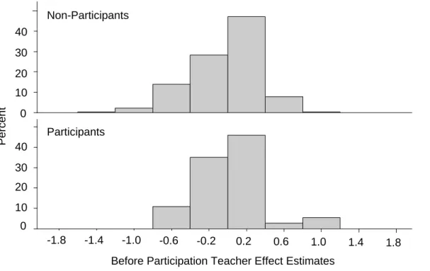
Figure43.1: Comparison of Before Participation Effects between Teachers Participating
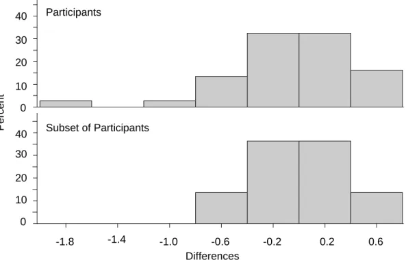
(n = 37) and Not Participating (n = 280) in M2 ... 57 Figure53.2: Comparison of Differences between Before and After Participation Effects
for MPS Teachers (n = 37) and a Subset of MPS Teachers (n = 22) Participating in M2 ... 58 Figure64.1: Visual of Cross-Classified Data Structure ... 65
Figure74.2: Level One Curve-of-Factors Model ... 66
Figure84.3: Comparison of ˆ
m iP
RMSE for the Curve-of-Factors (solid), CA Z-score (dash)
and MA Z-score (dotted) Models with Complete and Missing Tests, and MA/CA Z-score (dot-dash) Model with Missing Tests for Specific Percentiles and Years ... 77
Figure94.4: Comparison of ˆ
m iP
Bias for the Curve-of-Factors (solid), CA Z-score (dash)
and MA Z-score (dotted) Models with Complete and Missing Tests, and MA/CA Z-score (dot-dash) Model with Missing Tests for Specific Percentiles and Years ... 78
Figure104.5: Comparison across Years of the Estimated Sampling Distributions of ˆ p m ik P under the Curve-of-Factors (gray) and MA Z-score (black) Models with
Complete and Missing Tests for Teachers Truly at the 48th (solid) and 76th (dotted) Percentiles ... 80 Figure114.6: Comparison of the Estimated Probability of Classifying Teachers in the Upper Quartile for the Curve-of-Factors (solid), CA Z-score (dash) and MA Z-score (dotted) Models with Complete and Missing Tests, and MA/CA Z-score (dot-dash) Model with Missing Tests for Specific True Percentiles and Years .... 82
LIST OF TABLES
Table12.1: Comparison of Coefficient Matrices for Teacher Effects in Non-Layered and
Layered Models ... 19
Table22.2: Teacher Effect Estimates from NLM(0), NLM(0.7), LM(0) and LM(0.7) ... 31
Table33.1: Comparison of Z Matrix in Non-Layered and Layered Models ... 45
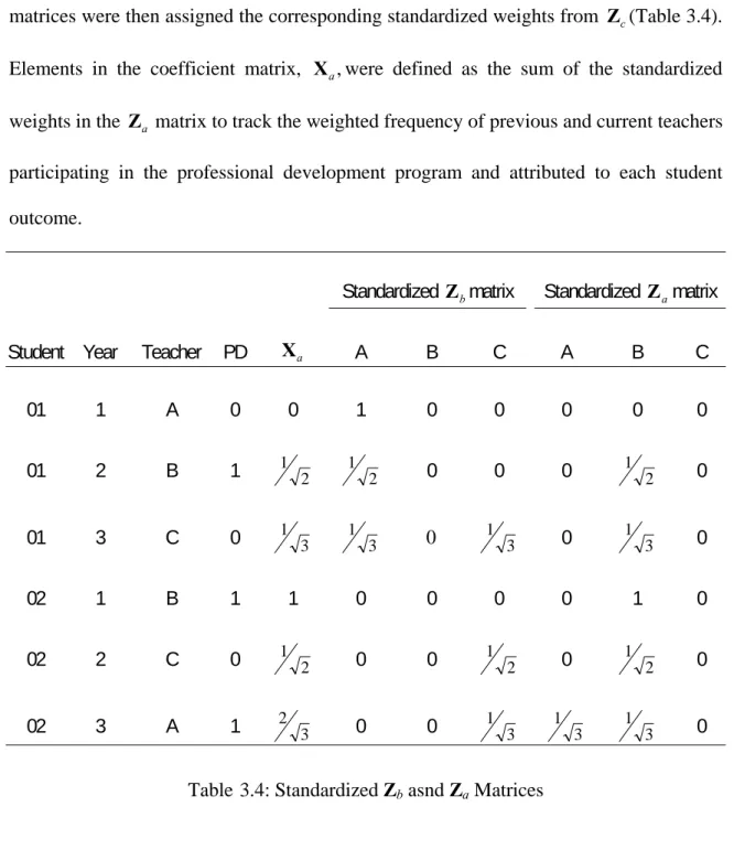
Table43.2: Zb and Za Matrices ... 47
Table53.3: Standardized Layered Z Matrix ... 49
Table63.4: Standardized Zb and Za Matrices ... 50
Table73.5: MPS Middle School Assessments between 2003-04 and 2007-08 ... 52
Table84.1: Comparison of Z Matrix in Non-Layered and Layered Models ... 69
Table94.2: MPS Middle School Assessments between 2003-04 and 2007-08 ... 70
Chapter 1
Introduction
Over the past several years, there has been a national effort to hold students to higher academic standards. This effort includes holding states accountable for assessing measurable student outcomes. Value-added modeling is an alternative approach to test-based accountability systems interested in the proportions of students scoring at or above pre-determined proficiency levels. Value-added modeling techniques estimate the contribution of educational factors, such as teachers, to growth in student achievement, while allowing for the possibility to control for the effect of non-educational factors beyond a school system’s control, such as socioeconomic status. Value-added modeling methods provide opportunities to estimate the proportion of variability in achievement or student growth attributable to teachers, as well as estimate an individual teacher’s effect on student learning.
School districts and policymakers desire to use teacher effect estimates for a variety of purposes, from informing educational systems how students are affected by current practices and conditions to making high-stakes decisions regarding teacher salary and/or employment. These estimates are also desired to evaluate the effectiveness of professional development programs. However, even though value-added modeling methods infer causal effects of teachers on student growth, the assessment data are not obtained from randomized, experimental studies. Consequently, several obstacles need to be addressed before value-added modeling should be used in these ways.
1.1 Value-Added Models for Estimating Teacher Effects
Chapter 2 serves as a background and introduction to value-added methodology. Several value-added models available for estimating teacher effects are described, as are the models’ respective advantages and disadvantages. Modeling variations, such as the use of layered versus non-layered design matrices and the specification of teacher effects as fixed or random, are also discussed, and the impact of such considerations on estimated teacher effects is explained in detail using an example provided by Wright and Sanders (2008). The various statistical and psychometric issues associated with estimating value-added teacher effects are highlighted, providing a summary of the current state of value-added modeling research and recommendations for future work.
1.2 Estimating the Impact of a Professional Development Program on Student Learning
Professional development programs focus on preparing teachers to meet the recent initiatives on improving the quality of student instruction, but rigorous evaluations are needed to determine whether these programs are actually effective. Value-added modeling techniques provide opportunities to estimate the relationship between teacher development and student learning, but most require student achievement data to be on a single developmental scale over time (McCaffrey, Lockwood, Koretz, & Hamilton, 2003). Typically, available assessment data do not meet such requirements, limiting analyses that can be conducted. Chapter 3 proposes alternative value-added methodology, specifically the use of Z-scores, for analyzing less-than-ideal longitudinal student achievement data collected from a mixture of norm- and criterion-referenced assessments to estimate the impact of a professional development program on student learning. The
chapter discusses methodology for estimating teacher effects on student learning before and after entering professional development and addresses issues arising when using a layered, longitudinal linear mixed model to analyze gains in standardized scores. The methodology is applied to data collected from a mathematics professional development program in mathematics education, the Math in the Middle Institute Partnership (M2), and the results are discussed.
1.3 Using Parallel Processing Methodology to Estimate Teacher Effects
Few studies have addressed how to use value-added models to analyze achievement data not on a single developmental scale (Green, Smith, Heaton, Jiao, & Stroup, under review; Rivkin, Hanushek, & Kain, 2005), and even fewer, perhaps none, have discussed how to use information from multiple instruments in a single year that are on different scales, potentially both within and between instruments over time. When modeling multiple outcome measures, instead of a single measure across time, parallel process, or multivariate, growth curve models can estimate the relationship between the growth trajectories for each of the parallel measures and allow researchers to investigate changes in latent factors over time instead of changes in observed scores. Chapter 4 describes the use of parallel processing, specifically curve-of-factors, methodology to analyze longitudinal student achievement data collected from two different assessments in a single subject, such as mathematics, and estimate teachers’ effects on student learning. Assuming data come from a curve-of-factors model structure, a simulation study evaluates the performance of the proposed curve-of-factors model in its ability to
accurately rank teachers in the presence of either complete or missing test data and compares it to the performance of the Z-score methodology proposed in Chapter 3.
Chapter 2
Value-Added Models for Estimating Teacher Effects
2.1 Introduction
Since the enactment of No Child Left Behind (NCLB) (2001), education systems, in theory, have held students to higher academic standards, and states are accountable for assessing measurable student outcomes. States receiving Title I funds for improving the academic achievement of disadvantaged students must require schools to make adequate yearly progress (AYP). While states are given latitude with regards to what is meant by “adequate,” in general, this means the proportion of students achieving pre-determined proficiency levels on state assessments is expected to increase annually until all students in particular grades are deemed proficient or higher.
Value-added modeling is an alternative approach to test-based accountability systems interested in the proportions of students scoring at or above pre-determined proficiency levels. Value-added modeling techniques estimate the contribution of educational factors, such as teachers, to growth in student achievement, while allowing for the possibility to control for the effect of non-educational factors beyond a school system’s control, such as socioeconomic status. Value-added modeling methods provide opportunities to estimate the proportion of variability in achievement or student growth attributable to teachers, as well as estimate an individual teacher’s effect on student learning. When these methods identify large differences in teacher effectiveness, they also have the potential to help researchers identify what characteristics highly effective
teachers possess and motivate informed improvements in education (McCaffrey, Lockwood, Koretz, & Hamilton, 2003).
Teacher effect estimates can be used for a variety of purposes, from informing educational systems how students are affected by current practices and conditions to making high-stakes decisions regarding teacher salary and/or employment. However, even though value-added modeling methods infer causal effects of teachers on student growth, the assessment data are not obtained from randomized, experimental studies.
Consequently, several limitations exist when defining what teacher effects really
describe. Defining teacher effects requires identifying to what a particular teacher’s impact on a student’s growth in achievement will be compared, such as other teachers in the school, district, or entire state. The definition also depends on the outcomes used to measure achievement; the scope and purpose of the instruments can limit what is measured and, consequently, restrict the part of a teacher’s total impact on a student that can be estimated (McCaffrey et al., 2003). Other factors affecting students’ growth in achievement, such as characteristics of classrooms and schools, can be confounded with teacher effect estimates, so the purpose for obtaining such estimates needs to be clearly defined and should dictate how precisely the effects need to be estimated. Typically, teacher effects merely account for unexplained classroom-level heterogeneity (Lockwood, McCaffrey, Mariano, & Setodji, 2007).
Studies investigating value-added teacher effects provide evidence teachers have differing effects on student learning (Rivkin, Hanushek, & Kain, 2005; Rowan, Correnti, & Miller, 2002; Wright, Horn, & Sanders, 1997) that persist over time (Sanders & Rivers, 1996), but these studies have shortcomings (McCaffrey et al., 2003). Section 2.2
describes proposed value-added models for estimating teacher effects and discusses their respective advantages and disadvantages. Section 2.3 covers the impact of different modeling decisions on the estimation of teacher effects, and Section 2.4 highlights various statistical and psychometric issues associated with estimating such effects. The chapter concludes with a summary of the current state of value-added modeling research and recommendations for future work.
2.2 Value-Added Models
Multiple authors have championed the use of value-added models to analyze longitudinal student achievement data (Doran, 2003; Drury & Doran, 2003; Hershberg, Simon, & Lea-Kruger, 2004; Lissitz, 2005; Sanders, Saxton, & Horn, 1997). These methods fall into three categories: covariate adjustment models, gain score models and multivariate models (McCaffrey et al., 2003).
2.2.1 Covariate Adjustment Models Covariate adjustment models, for example,
ig g g i ig ig y T e y , 1 , (2.1)
regress each student’s current achievement score, yig, on his or her prior score, yi,g1, for the year of data collection, g = 1, 2, 3, …, m. The student-specific mean, ig, adjusts for factors affecting a student’s level of achievement, such as free-and-reduced lunch and English Language Learner (ELL) identifiers. It can also account for many other factors, including characteristics of schools. The teacher effect, Tg, estimates the current year teacher’s impact on a student’s outcome. The residual errors, eig, are assumed to be
normally distributed with mean zero and variance eg2 and independent of the prior year scores and teacher effects.
Covariate adjustment models are easy to specify and fit, and they do not require performance on measures used in successive years to be placed on a single developmental scale so growth can be measured across grades or ages. This is particularly beneficial for school systems using a mixture of norm-referenced and/or criterion-referenced tests, where reported student scores from the two types of instruments reflect different measurements: either relative academic performance or proficiency on predetermined criteria, respectively. Teacher effects from prior years are embedded in the previous year’s score, so the effects persist indefinitely even though they are not explicitly specified in subsequent years’ models. However, information is lost about student performance by estimating models separately for each year, so critics argue these methods are not really measuring student growth. Covariate adjustment methods also require complete student records, so missing student outcomes must either be imputed or removed from the analysis. When data are not missing completely at random, list-wise deletion can lead to biased estimates of all effects. In general, covariate adjustment models are easy to work with, but potentially over-simplify the complexity of student growth over time.
2.2.2 Gain Score Models Gain score models,
ig g ig g i ig ig y y T e d , 1 , (2.2)
treat the difference between two successive scores, dig, for student i as the response for the gth year of data collection. The student-specific mean, ig, adjusts for factors
affecting a student’s growth from one year to the next. It can account for many factors, including characteristics of schools. The teacher effect, Tg, estimates the current year teacher’s impact on a student’s growth. The residual errors, eig, are assumed to be normally distributed with mean zero and variance eg2 and independent of the teacher effects.
Gain score models are also easy to specify and fit. These methods model students’ gains in scores, so time-invariant factors, such as gender, race and poverty level, affecting a student’s level of achievement need not be estimated. Prior year teacher effects are not typically specified in the model, which assumes they persist undiminished over time. Although “covariate” methods do not require tests to be on a single developmental scale, “gain” methods do, so changes in performance are not confounded with changes in tests (McCaffrey et al., 2003). In addition, gain score models require complete student records and lose information about student growth by assuming pairs of gains for the same student are independent. Overall, gain score models are easy to work with and explicitly model student growth in achievement, but they have stringent scale requirements and potentially over-simplify the complexity of student growth over time.
2.2.3 Multivariate Models
Multivariate methods jointly model all student scores, including relationships between each student’s set of outcomes. These approaches also accommodate missing data, making efficient use of all available information. Specifying a multivariate model provides more flexibility, allowing the exploration of several assumptions, such as the persistence of teacher effects and the residual covariance structure of student outcomes. In some instances, these models are robust to omitted covariates, but they are
computationally intensive and require much more in the way of computing resources than either the gain score or covariate adjustment methods. Even though multivariate methods are often recommended, they are not widely adopted because the required resources and high-quality longitudinal data are not readily available. Three common multivariate approaches include the cross-classified model (Raudenbush & Byrk, 2002), the Education
Value-Added Assessment System (EVAAS)teacher model (Sanders et al., 1997), and the
variable persistence model (McCaffrey, Lockwood, Koretz, Louis, & Hamilton, 2004). 2.2.3.1 Cross-Classified Models
Hierarchical linear models (HLMs) can model students’ growth over time, but when assessing teachers’ influence on rates of learning, the models require each outcome to belong to only one student, who in turn remains in a single teacher’s classroom over the course of the study (Raudenbush & Byrk, 2002). The nested structure required by HLMs is a limitation when studies want to model students’ growth over the course of several years and, subsequently, several teachers. Rather, students who share the same teacher(s) in one year do not share the same teacher(s) in the next year, resulting in a cross-classified structure (Rasbash & Browne, 2008; Raudenbush & Byrk, 2002); HLMs do not model this additional complexity.
Cross-classified models, for example,
0 0 0 1 0 1 1 2 0 1 2 2 3 0 1 2 3 3 2 3 i i i i i i i i i i i i i i i y m T e y m b T T e y m b T T T e y m b T T T T e , (2.3)model scores, yi,(g1), for student i at the g = 1, 2, 3, 4 year of data collection as a function of the average achievement, , and the average learning rate, . The
student-specific intercepts, mi, and slopes, bi, are assumed to be independent across students and normally distributed with mean zero, variances 0 and 1, respectively, and covariance
01
. The random teacher effects, Tk, are the expected deflections to students’ growth
curves when encountering teacher k. These effects are assumed to be independently,
normally distributed with mean zero and constant variance across years. Teacher effects are also assumed to be independent of all other effects in the model. The random errors,
ig
e , are assumed to be normally distributed and independent of each other, both within and between students, because the individual growth curves are assumed to “capture all the student-related influences on scores” (McCaffrey et al., 2003, p. 58).
More generally, the cross-classified model from above can be specified as,
1 ,( 1) ,( 1) ,( 1) 1 0 g K i g i i g i hik k i g k h y m a b D T e
, (2.4)where ai,(g1) assumes the value (g-1) at year g, and the term Dhik 1 if student i encounters teacher k at time h; 0Dhik otherwise. The teacher effects, Tk, are summed over time, so a student’s score is attributed to all previous and current teachers the student had for a particular subject. These types of models can also be extended to include other factors, such as student- and teacher-level covariates (Raudenbush & Byrk, 2002), as well as higher-order polynomials in g (Raudenbush, 2004).
Cross-classified models explicitly model individual growth curves, often using a linear trend instead of separate means for each year. The linear trend used to model student growth places restrictions on the residual error covariance matrix. Subsequently, whenever the covariance between mi and bi,01, is greater than zero, the variability of scores increases over time (McCaffrey et al., 2004). Raudenbush (2004) acknowledged
cross-classified approaches have stronger variance assumptions than models with unstructured variance-covariance matrices, but he argued this additional assumption potentially makes more appropriate and efficient use of student achievement data. Because cross-classified models can become complex quickly, other constraints may also need to be imposed to simplify a model.
In the cross-classified model described, teacher effects persist undiminished into the future, so contributions of past as well as current teachers, are accounted for in a student’s set of scores. Consequently, the variability due to teacher inherently increases with each additional year of data collection (McCaffrey et al., 2004). Scores must also be on a single developmental scale (McCaffrey et al., 2003).
2.2.3.2 EVAAS Model
One prominent multivariate longitudinal linear mixed model is the Education
Value-Added Assessment System (EVAAS) layered model (Sanders et al., 1997). This
approach assumes teacher effects are independent and persist undiminished over time and subject. For a single track of students within a school system, a simplified version of the EVAAS model for a particular subject, such as math or reading,
3 3 2 1 3 3 2 2 1 2 2 1 1 1 1 i i i i i i e T T T y e T T y e T y , (2.5)
models scores, yig, for student i at year g = 1, 2, 3 as a function of year-specific means,
g
. Random teacher effects are included for all teachers a student encounters for the
subject during the course of the study. The teacher effects are assumed to be normally distributed with zero mean and year-specific variances; these effects are assumed
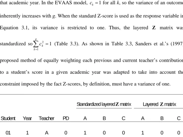
independent both within and across year. The random errors, eig, are assumed to be normally distributed and independent across students. Within-student correlations are assumed to follow an unstructured covariance structure with time-specific variances.
EVAAS jointly models more than one subject per grade for multiple cohorts of students across several school systems. The EVAAS teacher model (Sanders et al., 1997),
mk p p N p ijklmn ijkl m ijkl m iklm ijklmn c t e y 1 ) ( ) ( , (2.6)is much more complex, where yijklmn is the measurement on the nth student in the mth subject and the lth grade who encountered the jth teacher in the ith school system during the kth year. Separate fixed means, iklm, are estimated for each grade, year, subject and school system combination. The random effect of the jth teacher who taught in the ith school system during the kth year, lth grade and mth subject is tijklm, and cijklm is the fractional contribution of teacher j to the student’s score, accounting for instances when a student has multiple teachers for a subject in the same year. Finally, eijklmn, is the random deviation of the nth student’s measurement from the fixed mean.
The p p mijkl ijkl
m t
c ( ) ( ) terms are summed so a student’s score is attributed to all
previous and current teachers the student had for subject m, creating a layered model. The teacher effects are summed over the index p, which tracks the student across years and allows for multiple teachers in the same year. The total number of teachers a student had though year k in subject m is Nmk.
The random teacher effects are assumed independent across teacher, subject, grade and time, even when the same teacher teaches multiple subjects, grades and/or
years. Separate teacher variance components are estimated for each year, subject and grade combination, creating a heterogeneous, diagonal variance-covariance matrix for the random teacher effects. The EVAAS teacher model also uses an unstructured variance-covariance matrix to account for relationships between each student’s set of scores across subjects and grades, but assumes different students’ scores are independent. Teachers’ impact is analyzed based on at least three years of student data (Sanders et al., 1997).
In both the cross-classified and the EVAAS teacher models, teacher effects persist undiminished into the future, so contributions of both current teachers and past teachers are accounted for in a student’s set of scores. Consequently, the total teacher contribution to the variability of scores increases over time, even though the total variance may not, depending on the testing instrument used (McCaffrey et al., 2004). However, the EVAAS model, unlike the cross-classified model, does not place restrictions on the overall grade-specific means or the covariance structure of repeated measurements on the same student (McCaffrey et al., 2004; Wright, Sanders, & Rivers, 2006). The unstructured within-student covariance matrix allows each within-student to serve as his or her own control, making it unnecessary to account for factors affecting a student’s level of achievement (Sanders et al., 1997). Yet, both of these models are computationally intensive and require scores be on a single developmental scale (McCaffrey et al., 2003).
2.2.3.3 Variable Persistence Model
McCaffrey et al. (2004) proposed the variable persistence model, a generalized version of multivariate longitudinal models for student outcomes. This approach is similar to the EVAAS teacher model, but it allows prior teachers to have variable contributions to current scores rather than assuming complete persistence of these effects.
For a single track of students within a school system, a simplified version of the variable persistence model for a particular subject,
3 3 2 32 1 31 3 3 2 2 1 21 2 2 1 1 1 1 i i i i i i e T T T y e T T y e T y , (2.7)
models scores, yig, for student i at year g = 1, 2, 3 as a function of year-specific means,
g
. Random teacher effects are included for all teachers a student encounters for the
subject during the course of the study. The teacher effects are assumed to be normally distributed with zero mean and year-specific variances; these effects are assumed independent both within and across year. The persistence of prior teacher t on subsequent scores at year g is gt, which is estimated. The random errors, eig, are assumed to be normally distributed and independent across students. Within-student correlations are estimated using an unstructured covariance structure with time-specific variances.
The variable persistence model can be extended to include student- and school-level covariates (McCaffrey et al., 2003). A special case of the variable persistence model (Lockwood, McCaffrey, Mariano, et al., 2007),
ig g ig g g gg ig g g ig e y
* ' * * * ' θ φ x β , (2.8)includes covariates, but not school effects, where yig is student i’s score in year g, g = 1, 2, …, m, and g is the year-specific mean. Time-invariant and time-varying covariates for student i are included in the vector, xig. The random teacher effects for each year,
g
θ , are linked to students by φig, which allows fractional contributions of teachers to student i’s score during year g. The persistency parameters, gg*, model the strength of
past teacher effects on current student measurements, where gg* 1 when g* = g. The
term eig represents random error. Similar to the EVAAS teacher model, the variable
persistence model can be extended to account for multiple cohorts of students, subjects per grade and school systems, but the model quickly grows in complexity (Lockwood, McCaffrey, Mariano, et al., 2007).
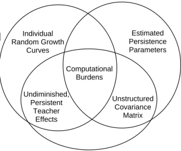
Although the variable persistence model allows teacher effects to persist into the future, it does not assume these effects persist undiminished. Instead, the persistency parameters are freely estimated, so the total teacher contribution to the variability of scores does not inherently increase over time, unlike the cross-classified and EVAAS teacher models (McCaffrey et al., 2004). However, as the persistency parameters approach zero, correlations between future scores of students who shared a teacher in the past are no longer accounted for, eliminating one of the benefits of using the layered modeling approach (Wright & Sanders, 2008). In fact, McCaffrey et al. (2004) and Lockwood, McCaffrey, Mariano, et al. (2007) found estimated teacher effect persistency parameters to be relatively small.
McCaffrey et al. (2004) showed, under certain restrictions, each of the alternative value-added modeling approaches discussed is a special case of the general, variable persistence model (Figure 2.1). Although the multivariate methods allow efficient use of all available data and are typically recommended, they are computationally intensive and require much more in the way of computing resources than either the gain score or
covariate adjustment methods. While similar in many regards, each of the multivariate
omputationally intensive and require much more in the way of computing resources than either the gain score or covariate adjustment methods.
Without covariates, gain scores and the cross-classified model are special cases of the layered model with restrictions to the overall time trend and/or the distribution of residual errors. The layered model is a special case of the general model with restrictions to the αs and without covariates. The covariate adjustment and gain-score model with covariates are special cases of the general model with restrictions to the distribution of residual errors and the αs.
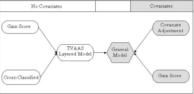
Note. From “Models for Value-Added Modeling of Teacher Effects,” by D. F. McCaffrey, J. R. Lockwood, D. Koretz, T.A. Louis, and L. Hamilton, 2004, Journal of Educational and Behavioral Statistics, 29(1), p. 78. Copyright 2004 by Sage Publications, Inc. Adapted with permission. McCaffrey et al. (2004) refer to the EVAAS layered model as the TVAAS layered model.
Figure12.1: Relationship among Models
the variable persistence models, the cross-classified framework models individual growth curves for students, so its within-student covariance matrix is restricted. Also, while both the cross-classified and EVAAS teacher models assume teacher effects persist undiminished in the future, the variable persistence model allows the strength of these effects on future scores to vary. Consequently, the variable persistence model only requires scores be linearly related instead of on a single developmental scale (McCaffrey et al., 2004): that is, the cumulative distribution functions for different scales should not cross (McCaffrey et al., 2003). While the additional complexities of these modeling
approaches can be beneficial, they also come with the price of additional computational burdens.
Figure22.2: Comparison of Multivariate Models for Modeling Longitudinal Student
Achievement Data
2.3 Estimating Teacher Effects
Studies investigating value-added teacher effects provide evidence teachers have differing effects on student learning (Rivkin et al., 2005; Rowan et al., 2002; Wright et al., 1997) that persist over time (Sanders & Rivers, 1996), but these studies have shortcomings. Statistical and psychometric issues arise when estimating teacher effects using longitudinal student achievement data (McCaffrey et al., 2003). Different modeling variations, such as the use of layered versus non-layered design matrices and the estimation of random versus fixed teacher effects, are described, and the impact of such considerations on estimated teacher effects follows.
Estimated Persistence Parameters Undiminished, Persistent Teacher Effects Individual Random Growth Curves Unstructured Covariance Matrix Computational Burdens
Cross-Classified
Model
Variable
Persistence
Model
EVAAS Model
2.3.1 Layered Models
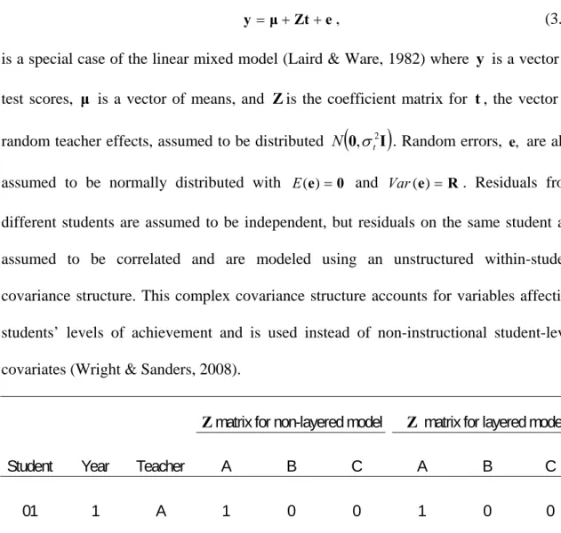
Wright and Sanders (2008) distinguish between the layered and non-layered model in the construction of the coefficient matrix for teacher effects (Table 2.1). In the non-layered model, each student’s outcome in a given year is linked only to the current teacher. In contrast, the layered model links a student’s achievement to current and previous teachers within a given time span. Therefore, the coefficient matrix for the layered model can have several “1”s in a row, connecting past teachers with subsequent student outcomes. This approach accounts for the “correlation of future scores for students who [have] shared a past teacher” (Lockwood, McCaffrey, Mariano, et al., 2007, p. 126).
Matrix for non-layered model Matrix for layered model Student Year Teacher A B C A B C
01 1 A 1 0 0 1 0 0 01 2 B 0 1 0 1 1 0 01 3 C 0 0 1 1 1 1 02 1 B 0 1 0 0 1 0 02 2 C 0 0 1 0 1 1 02 3 A 1 0 0 1 1 1
Note. The example used estimates one overall teacher effect for each teacher instead of a separate teacher effect for each year.
Table12.1: Comparison of Coefficient Matrices for Teacher Effects in Non-Layered and
2.3.2 Best Linear Unbiased Predictors
Teacher effects may be specified as either fixed or random effects depending on the intended scope of inference. If teacher effects are treated as fixed, the underlying assumption is the observed teachers are the only units of interest; conclusions drawn apply only to the teachers for whom data were collected. If teacher effects are specified as random, it is assumed the observed teachers represent a random sample from a population of teachers to which conclusions can be applied. Random teacher effects are estimated by best linear unbiased predictors (BLUPs), which are also referred to as shrinkage estimators (Raudenbush & Byrk, 2002; Robinson, 1991). This estimation procedure weights the average deviations of each teacher’s students’ scores from the overall average score. The weighting takes into account sample size and variability within, as well as across, teachers’ classrooms to “shrink” teacher effect estimates to the overall mean of the distribution of teacher effects, assumed to be zero. Each teacher’s random effect is estimated relative to all other teachers in the sample, and the variability of the estimated teacher effects is assumed to represent variability present in the population of teachers. Such shrinkage and relative estimation does not occur in the estimation of fixed effects.
2.3.3 Impact of Model Specification on Teacher Effect Estimates
Wright and Sanders (2008) explain the EVAAS model in further detail by comparing it to three other sub-models. The researchers use simple examples to illustrate the effect layered design matrices and/or within-student correlations have on estimated teacher effects. In these examples, Wright and Sanders (2008) use a special case of the linear mixed model (Laird & Ware, 1982),
e Zu Xβ
y , (2.9)
where y is a vector of test scores, X tracks the year of each test score, β is a vector of overall mean scores for each year and Zis the coefficient matrix for u, the vector of
random teacher effects, assumed to be normally distributed with E(u)0 and
, )
( txt 2 t
Var u D I where t is the total number of teachers. Random errors, e, are also
assumed to be normally distributed with E(e)0,
0 2 2 2 2 2 2 2 2 2 2 ) (e R I R n ns x ns
Var and ,Cov(u,e)0 where n is
the number of students with test scores and s is the number of test scores for each student; residuals from different students are assumed to be independent, but measures on the same student are assumed to be correlated. The overall variance of test scores is
, ) (y ZDZ R 2 ZZ R0 2V0 VVar T T where 2 2 . Variancecomponents are not estimated from the data, because the focus is on the estimation of fixed means and random teacher effects. In each of the examples, the ratio of teacher variance to residual variance, , is fixed at 1000 to reduce the amount of shrinkage in the teacher effect estimates and, subsequently, make the estimates easier to interpret; the within-student correlation, ,is specified as either 0 or 0.7. Substituting V0for ,V R0 for R and Itfor D in the estimating equations for fixed and random effects does not change the estimates produced.
One of the examples involves three years of scores for nine different students (Figure 2.3). These data can also be found in Table 10 of Wright and Sanders (2008). In
1 2 3 300 400 500 600 700 300 400 500 600 700 300 400 500 600 700 1 2 3 1 2 3 D G H
Track 1, Teacher B Track 2, Teacher C
A D E E G H B C E D E D H H G G F J Year Score Track 1, Teacher A
each year there are three different teachers: teachers A, B and C in year one; teachers D, E and F in year two; and teachers G, H and J in year three. As shown in Figure 2.3, the teachers fall into two different tracks: students who have teacher A or B in year one do not share any teachers over the course of the three years with the student who has teacher C in year one; students who have teacher A or B in year one either have teacher D or E in year two and teacher G or H in year three, whereas the student who has teacher C in year one has teachers F and J in years two and three, respectively. Subsequently, the estimated random effects of teachers depend on deviations for students in the teachers’ respective tracks, where deviations are the differences between students’ scores and the corresponding yearly mean. The students’ scores are also assumed to be scaled so changes in scores from year to year are meaningful.
Figure32.3: Student Scores and Teachers over Time
Estimates of random teacher effects are compared for four different models: 1) the
non-layered model (NLM) with within-student correlations set to zero ( 0),
the layered model (LM) with 0, abbreviated LM(0); and 4) the layered model with , 7 . 0
abbreviated LM(0.7). For the previously described data, Wright and Sanders
(2008) provide formulas for calculating the effects of the second and third year teachers using each of the four models. Estimated teacher effects during the first year are not value-added and, while estimated, are not discussed; students do not have previous scores from which to determine the value a year one teacher has added. In the formulas, “M” represents the mean of the deviation scores
yXβ
for a group of students, the subsequent integer indicates the year for which the deviations were calculated and the subscript denotes the students’ corresponding teacher(s). For example, M2D representsthe average year two deviation score of students taught by teacher D, and M1DE
represents the average year one deviation score of students taught by teachers D and E in year two. Differences in teacher effect estimating equations for the four models are discussed using this notation.
The NLM(0) teacher effect estimates are merely unadjusted means of students’ deviation scores. For instance, the estimated random effect of teacher D in year two is the mean deviation score of students taught by teacher D during year two,
M2D = Σ(Score – Year Two Fixed Effect Mean) / Number of Students
= {(440 – 500) + (380 – 500) + (500 – 500) + (440 – 500)} / 4 = -60.
Similarly, the estimated random effect of teacher G is the average deviation score of the students he or she taught in year three,
= {(470 – 600) + (550 – 600) + (530 – 600) + (610 – 600)} / 4 = -60.
The NLM(0) estimates do not incorporate expected deviation scores, because within-student correlations are assumed to be zero; no basis exists for which to obtain such expected deviations. Consequently, teachers with generally higher achieving students will appear to be more effective than teachers with generally lower achieving students, even when the latter have huge impacts on their students’ learning.
The NLM(0.7) teacher effect estimates adjust the means of students’ deviation scores in a given year to account for students’ deviation scores in other years, as in analysis of covariance (ANCOVA). For example, the estimated random effect of teacher D in year two is the mean deviation score of students taught by that teacher during that time adjusted by the students’ expected deviation scores. The formula,
M2D – b(M1D – M1DE) – b(M3D – M3DE),
can be interpreted in three parts: M2D, b(M1D – M1DE) and b(M3D – M3DE). The mean
deviation score of students taught by teacher D in year two, M2D, is -60; this is the
NLM(0) estimate for teacher D.
However, M2D is adjusted by the expected year one deviation score for students
taught by teacher D in year two, b(M1D – M1DE). The coefficient, b, is the pooled
within-teacher multiple regression coefficient for predicting students’ year two deviation scores from their corresponding year one and year three deviation scores. In this example, b = / (1 + ) = 0.7 / (1 + 0.7) = 0.411765. The mean year one deviation score of students taught by teacher D in year two is:
M1D = Σ(Year One Score for Students Taught by Teacher D – Year One Fixed
Effect Mean) / Number of Students
= {(370 – 400) + (350 – 400) + (430 – 400) + (410 – 400)} / 4 = -10.
The expected year one deviation score also incorporates the mean year one deviation score of students taught by teacher D or E in year two,
M1DE = {Σ(Year One Score for Students Taught by Teacher D – Year One Fixed
Effect Mean) + Σ(Year One Score for Students Taught by Teacher E – Year One Fixed Effect Mean) } / Number of Students
= {(370 – 400) + … + (410 – 400) + (330 – 400) + …. + (370 – 400)} / 8 = -30.
Hence, the students taught by teacher D in year two had an above-average deviation score in year one, b(M1D – M1DE) = 0.411765{(-10) – (-30)} = 8.235.
The mean, M2D, is also adjusted by the expected year three deviation score for
students taught by teacher D in year two, b(M3D – M3DE). The mean year three deviation
score of students taught by teacher D in year two is:
M3D = Σ(Year Three Score for Students Taught by Teacher D – Year Three
Fixed Effect Mean) / Number of Students
= {(470 – 600) + (530 – 600) + (530 – 600) + (590 – 600)} / 4 = -70.
This mean is then compared to the mean year three deviation score of students taught by teacher D or E in year two,
M3DE = {Σ(Year Three Score for Students Taught by Teacher D – Year Three
Fixed Effect Mean) + Σ(Year Three Score for Students Taught by Teacher E – Year Three Fixed Effect Mean) } / Number of Students
= {(470 – 600) + … + (590 – 600) + (550 – 600) + …. + (670 – 600)} / 8 = -30,
to produce an expected year three deviation score of 0.411765{(-70) – (-30)} = -16.471. Together, these three parts comprise the NLM(0.7) estimate for the random effect of teacher D in year two:
M2D – b(M1D – M1DE) – b(M3D – M3DE)
= -60 – 0. 411765{(-10) – (-30)} – 0.411765{(-70) – (-30)} = -60 – 0. 411765{20} – 0.411765{-40}
= -51.8.
Although slightly higher than teacher D’s NLM(0) estimate of -60, the estimate of -51.8 still indicates teacher D had a lower than average teacher effect. The NLM(0.7) estimate is simply an adjusted mean of the students’ deviation scores. Although the adjustments based on expected deviations are conventional, some properties of these adjustments are undesirable. For instance, future scores are used to adjust for earlier scores, even though the covariate is potentially affected by the prior year teacher; this is typically inappropriate for ANCOVA and may also be inappropriate in this context. The NLM(0.7) estimate for the effect of teacher D uses the students’ third year deviation scores to adjust for their second year deviation scores, even though teacher D’s impact may also affect student performance in year three. Additionally, the NLM(0.7) estimates reduce a
teacher’s effect if his or her students’ subsequent deviation scores are above-average, i.e., a teacher is penalized if students go on to have higher than expected gains.
The NLM(0.7) estimates are also susceptible to within-track centering of the covariates. The expected deviation scores are found by comparing a teacher’s mean student deviation score to the mean deviation scores of students in the same track rather than the mean deviation scores of all students for whom scores are available. For example, the NLM(0.7) estimate for teacher D uses M1DE and M3DE to center the year
one and year three covariates, respectively. Teacher D and E’s students are not in the same track as teacher F’s student. Consequently, the year one and year three deviation scores of teacher F’s student do not impact the centering of the covariates for estimating teacher D and teacher E’s NLM(0.7) effects. Although these scores are included in the estimation of the year one and year three fixed effect means, the fixed effect means used in the calculation of M1D, M1DE, M3D and M3DE cancel when finding the differences
(M1D – M1DE) and (M3D – M3DE). Therefore, teacher F’s student deviation scores do not
affect the NLM(0.7) estimates of teacher D and E’s effects. Similarly, when estimating the NLM(0.7) effect for teacher F in year two, the year one and year three mean deviation scores are found for only the students in that same track. This example is particularly problematic, because the within-track centering of the covariates simplifies the formula for this estimate,
M2F – b(M1F – M1F) – b(M3F – M3F),
to be merely the unadjusted mean deviation score for teacher F’s student in year two, M2F, the same as the NLM(0) estimate; no adjustments are made, because the expected
In year three, the NLM(0.7) estimates have similar issues. The estimated effect for teacher G in year three,
M3G – b(M2G – M2GH) – b(M1G – M1GH),
is the mean deviation score for teacher G’s students in year three, M3G, adjusted for the
students’ performance in years one and two, b(M1G – M1GH) and b(M2G – M2GH),
respectively. Although the covariates for years one and two are not affected by the year three deviation scores, the year three NLM(0.7) estimates are still susceptible to within-track centering. Consequently, the NLM(0.7) estimates for teachers F and J do not account for the student’s previous performance and, therefore, are not truly value-added effects.
The LM(0) teacher effect estimates are also adjusted means, but the estimates incorporate between-track differences and between-student correlations. For instance, the random effect of teacher D in year two is estimated using
M2D – M1DE + 0.5[(M3D – M3DE) – (M2D – M2DE)].
The mean deviation score of students taught by teacher D in year two, M2D = -60, is
adjusted by the mean year one deviation score for students taught by either teacher D or E
in year two, M1DE = -30, and the performance of teacher D’s students in year three
compared to year two, relative to students on the same track, 0.5[(M3D – M3DE) – (M2D –
M2DE)] = 0.5[{(-70) – (-30)} – {(-60) – (-30)}] = -0.5. Together, these adjustments
produce the estimated LM(0) effect for teacher D in year two, -35, which is higher than the NLM(0) estimate of -60, but still below the average teacher effect. The LM(0) effect for teacher F in year two simplifies to be
because this track consists of only one teacher in each year, nullifying the adjustment for future scores and reducing the teacher effect to simply a mean gain. However, in both of these estimates, the LM(0) effects account for between-track differences, unlike the NLM(0.7) estimates. The mean deviation of the previous year’s scores is track specific, but it incorporates the fixed effect mean for that year, which is estimated using data from all students, irrespective of track. This is contrary to the NLM(0.7) estimates, in which each fixed effect mean cancels due to the centering of each covariate.
The LM(0) estimates also account for the between-student correlations induced by using the layered design matrix. Expected deviation scores are found based on deviation scores for students who have shared at least one common teacher. In the adjustment for teacher D’s effect, 0.5[(M3D – M3DE) – (M2D – M2DE)], teacher D is rewarded if his or
her students perform better in year three than they did in year two, relative to other students on the same track. Likewise, if teacher D’s students have relatively worse future performance, his or her teacher effect estimate decreases; this is contrary to the estimation of the NLM(0.7) teacher effects. Although no future scores are available to obtain this type of adjustment for year three LM(0) teacher effect estimates, between-student correlations are accounted for through the additional prior year adjustment in the teacher effect estimates. For instance, the formula for the LM(0) estimate for teacher G in year three is M3G – M2GH, where M2GH adjusts the year three mean deviation score for
teacher G, M3G, by accounting for prior mean score deviations, between-track differences
and between-student correlations. This type of adjustment also occurs in the year two LM(0) teacher effect estimates (e.g., M1DE for teacher D’s effect and M1F for teacher F’s
correlations, so expected deviations scores for a student cannot be based on other scores from the same student, only on scores of students who have shared the same teacher(s).
The LM(0.7) estimates account for both between- and within-student correlations. The LM(0.7) random effect of teacher D in year two is estimated using
M2D – M1DE – 0.7(M1D – M1DE) + 0.5[(M3D – M3DE) – (M2D – M2DE)],
which is similar to the LM(0) estimate. However, the LM(0.7) utilizes within-student correlations to obtain expected deviation scores for students based on other scores from those same students. The inclusion of the additional term, 0.7(M1D – M1DE), compares
the mean year one deviation score for students who had teacher D in year two to the mean year one deviation score for students in the same track. The LM(0.7) estimate for teacher G in year three,
M3G – M2GH – b(M2G – M2GH) – b(M1G – M1GH),
also accounts for within-student correlations by incorporating the students’ prior mean deviation scores in both year one, b(M1G – M1GH), and year two, b(M2G – M2GH). By
making use of both between- and within-student information, the LM(0.7) teacher effect estimates utilize expected deviation scores based on scores of students who have shared the same teacher(s), as well as other scores from the same student.
Table 2.2 displays the year two and year three teacher effect estimates from each of the four models discussed using the student scores graphed in Figure 2.3. Estimates are not included for year one teachers A, B and C, because their effect estimates cannot be described as value-added. However, comparing the year two and year three teacher effect estimates is particularly enlightening. As illustrated in Figure 2.3, student gains from year one to year two and from year two to year three support the notion teachers E and H had
relatively higher than average effects on student learning. Alternatively, the effects of teachers D and G on student gains from one year to the next were below average, while the effects of teachers F and J were average. The effects of teachers G and H are further magnified by considering each student’s score trajectory from year one to year two through the inclusion of within-student correlations; the students’ trajectories drastically change after teacher G’s and teacher H’s instruction, whereas the trajectory for teacher J’s student does not change.
Model Year Teacher NLM(0) NLM(0.7) LM(0) LM(0.7) 2 D -60 -51.8 -35 -49 E 0 -8.2 35 49 F 60 60 0 0 3 G -60 -76.5 -30 -46.5 H 0 16.5 30 46.5 J 60 60 0 0
Table22.2: Teacher Effect Estimates from NLM(0), NLM(0.7), LM(0) and LM(0.7)
The non-layered models produce estimates reflecting mean deviation scores; NLM(0) estimates are merely unadjusted mean deviation scores, while NLM(0.7) are mean deviation scores adjusted for students’ prior and/or future achievement. Consequently, the teacher effect estimates for these models portray teachers F and J as highly effective teachers, simply because their student had higher than average scores in years two and three, not because the student showed higher than average growth.
Alternatively, the layered models produce estimates reflecting mean gains in deviation scores. As a result, teachers F and J had teacher effect estimates of zero for both layered models, because their student had relatively average mean gains and the student’s score trajectory did not change over time; the estimate of zero conveys the teacher did not have a value-added effect on the student’s learning. Additionally, accounting for within-student correlations provides more information about within-student growth over time, pulling the other LM(0.7) teacher effect estimates further from zero than the LM(0) estimates for the same teachers.
The variable persistence model (Equation 2.8) proposed by McCaffrey et al. (2004) allows teacher persistency parameters to vary. However, estimated persistency parameters tend to be near zero (Lockwood, McCaffrey, Mariano, et al., 2007; McCaffrey et al., 2004), so the teacher effect estimates from the low-persistency model approach the undesirable behavior of the NLM(0.7) estimates and do not appear to be value-added; estimates fail to account for between-track differences, and teachers are penalized for students who perform unexpectedly well in future years. As discussed by McCaffrey et al. (2004), the non-layered and low-persistency model estimates are also typically more susceptible to bias from omitted variables correlated with the level of student achievement than are the layered model estimates. In fact, the risk of overcorrecting teacher effects arises if non-instructional, time-invariant covariates beyond a school system’s control, such as race and poverty status, are included in the layered model. However, teacher effect estimates are susceptible to bias if variables correlated with gains in student achievement are omitted, irrespective of how teacher effect persistency is or is not specified.
In general, using the EVAAS layered model (Equation 2.6) to estimate teacher effects has advantages over other modeling approaches. The layered model accounts for both between- and within-student correlations to adjust for past and future student achievement scores. The model also uses all available scores, resulting in “less biased, more stable, more efficient estimates” (Wright & Sanders, 2008, p. 14) than either the gain score (Equation 2.2) or the covariate adjustment model (Equation 2.1). The use of multiple years of data allows estimates to be adjusted, thereby accounting for external pulses occurring in a given year and rewarding teachers whose students perform better than expected in the future. Overall, Wright and Sanders (2008) argue the EVAAS layered model is a competitive option for estimating teacher effects, because of its flexibility and adherence to value-added philosophy.
2.4 Issues
Uncertainty remains concerning whether student background variables should be included as covariates. The EVAAS model does not include such covariates, but researchers can inappropriately extend this practice to other, less sophisticated longitudinal value-added models. Instead, decisions to model student-level covariates should be based upon the interaction of several factors: “the distribution across classes and schools of students with different characteristics, the relationship between the characteristics and outcomes, the relationship between the characteristics and true teacher effects, and the type of model used” (McCaffrey et al., 2003, p. 70). Bias of teacher effect estimates is an issue when students are disproportionately assigned to schools and/or classrooms based on background characteristics related to student outcomes and true
teacher effects. When student background characteristics are correlated with teacher effects, the inclusion of student-level covariates can mask the effects of teachers. Fixed effects estimation of the covariates overcorrects for these background characteristics and results in underestimation of true, random teacher effects. For example, if highly effective teachers are assigned to affluent students, socioeconomic status becomes a proxy for teacher quality and true teacher effects are underestimated. Ballou, Sanders, and Wright (2004) propose a strategy to adjust for bias when student characteristics are correlated with true teacher effects, but strategies to address the issue of bias resulting from contextual effects as a result of aggregate-level variables have yet to be developed. Ultimately, when deciding whether to control for covariates, researchers must choose between potentially confounding teacher effects with student-level variables and potentially biasing teacher effects.
Debates also continue about the persistency of teacher effects. The EVAAS (Equation 2.6) and cross-classified models (Equation 2.4) assume teacher effects persist undiminished into the future. As a result, prior teachers affect a student’s score in a particular year, but not a student’s gain in scores from one year to the next. Gain score models (Equation 2.2) implicitly make the same assumption in that gains do not rely on prior year teacher effects. Consequently, the models assume teachers do not affect students’ future growth. In the variable persistence model (Equation 2.8), however, student gains depend on prior teachers’ effects, because the differences between the current and previous year’s persistency parameters for teacher effects are not necessarily zero, as they are in complete persistence models. Similarly, covariate adjustment models (Equation 2.1) assume prior teacher effects influence student growth at the rates specified
by the coefficients for prior scores. Yet, the potential advantages of freely estimating persistency parameters need to be carefully weighed against the advantages of using a layered model; as the persistency parameters approach zero, correlations between future scores of students who shared a teacher in the past are no longer accounted for, eliminating one of the benefits of using the layered modeling approach (Wright & Sanders, 2008).
Other issues arise when linking teachers to student scores. In some cases, students have incomplete records, missing some or all of their teacher links in a given year. This can occur when students are taught by multiple teachers in a single subject. Specifically, students may transfer to different schools midyear, be team-taught and/or learn a subject, such as reading, in multiple teachers’ classes. Such instances result in complex teacher links, and linking a student’s outcome to only one (or even no) teacher in a particular year may confound an identified teacher’s effect with other, unidentified teachers’ effects. However, determining how to accurately reflect the effect of multiple teachers on a student is not straightforward and requires potentially unrealistic assumptions.
Issues associated with the construction and scaling of instruments used to measure student achievement also exist. Typically, measures of student achievement are assumed to be on an interval scale, where any difference in scores has the same meaning at any point on the scale. For example, a student with test scores of 40 and 60 in consecutive years is assumed to have made the same amount of growth as a student with scores of 20 and 40. However, linking scores from different tests to a single scale for comparisons across grades may require nonlinear transformations, where rates of growth no longer have the same meaning across all ability levels. As illustrated in the previous example,