This is a repository copy of
Collaborative Multi-Objective Optimization for Distributed
Design of Complex Products
.
White Rose Research Online URL for this paper:
http://eprints.whiterose.ac.uk/129994/
Version: Accepted Version
Proceedings Paper:
Duro, J., Yan, Y., Purshouse, R. orcid.org/0000-0001-5880-1925 et al. (1 more author)
(2018) Collaborative Multi-Objective Optimization for Distributed Design of Complex
Products. In: Proceedings of the Genetic and Evolutionary Computation Conference 2018.
GECCO '18 Genetic and Evolutionary Computation Conference, 15-19 Jul 2018, Kyoto.
ACM . ISBN 978-1-4503-5618-3
https://doi.org/10.1145/3205455.3205579
[email protected]
https://eprints.whiterose.ac.uk/
Reuse
Items deposited in White Rose Research Online are protected by copyright, with all rights reserved unless
indicated otherwise. They may be downloaded and/or printed for private study, or other acts as permitted by
national copyright laws. The publisher or other rights holders may allow further reproduction and re-use of
the full text version. This is indicated by the licence information on the White Rose Research Online record
for the item.
Takedown
If you consider content in White Rose Research Online to be in breach of UK law, please notify us by
Design of Complex Products
João A. Duro
Department of Automatic Control & Systems Engineering, University of Sheffield, UK
Yiming Yan
Department of Automatic Control & Systems Engineering, University of Sheffield, UK
Robin C. Purshouse
Department of Automatic Control & Systems Engineering, University of Sheffield, UK
Peter J. Fleming
Department of Automatic Control & Systems Engineering, University of Sheffield, UK
ABSTRACT
Multidisciplinary design optimization problems with competing objectives that involve several interacting components can be called complex systems. Nowadays, it is common to partition the opti-mization problem of a complex system into smaller subsystems, each with a subproblem, in part because it is too difficult to deal with the problem all-at-once. Such an approach is suitable for large organisations where each subsystem can have its own (specialised) design team. However, this requires a design process that facili-tates collaboration, and decision making, in an environment where teams may exchange limited information about their own designs, and also where the design teams work at different rates, have dif-ferent time schedules, and are normally not co-located. A multi-objective optimization methodology to address these features is described. Subsystems exchange information about their own op-timal solutions on a peer-to-peer basis, and the methodology en-ables convergence to a set of optimal solutions that satisfy the over-all system. This is demonstrated on an example problem where the methodology is shown to perform as well as the ideal, but “unreal-istic” approach, that treats the optimization problem all-at-once.
CCS CONCEPTS
•Computing methodologies→Search methodologies; Co-operation and coordination;Modeling and simulation; • Ap-plied computing→Multi-criterion optimization and decision-making;
KEYWORDS
Collaborative multidisciplinary optimization, Complex systems, Multi-objective evolutionary algorithms, Multiple-criteria decision-making ACM Reference Format:
João A. Duro, Yiming Yan, Robin C. Purshouse, and Peter J. Fleming. 2018. Collaborative Multi-Objective Optimization for Distributed Design of Com-plex Products. InGECCO ’18: Genetic and Evolutionary Computation Con-ference, July 15–19, 2018, Kyoto, Japan.ACM, New York, NY, USA, 8 pages.
1
INTRODUCTION
The design of a large complex engineering system, such as an au-tomotive vehicle, usually involves the design of multiple individ-ual subsystems (or components), often mutindivid-ually interdependent.
Other terms used to refer to such systems includesystems of sys-tems[6] andinterwoven systems[5]. For such a complex design, it is common for organisations to assign individual design teams to each subsystem, often arranged along disciplinary lines or a com-pany’s own organisation structure, where each team has its own specific expertise on a particular science or engineering discipline. This requires the design teams to collaborate, but often the teams work at different speeds, have different time schedules and differ-ent work locations. Each design team is expected to satisfy multi-ple design criteria.
It is often the case that the subsystems are coupled, which means, for example, that there are (shared) design variables controlled by more than one subsystem at a time. The existence of interactions between the subsystems thus makes it difficult to predict the be-haviour of the entire system. Also, the design of such systems is frustrated by conflicting demands when attempts are made to sat-isfy the multiple criteria of all of the subsystems simultaneously.
This paper presents a methodology to support collaborative multi-objective optimization for the distributed design of complex prod-ucts. The remainder of the paper is organised as follows. Section 2 describes related literature and presents the novelty of the pro-posed methodology. In Section 3, a simple representative model of a complex system is presented, which consists of two interacting subsystems where each subsystem is modelled as a multi-objective optimization problem. A new methodology for distributed multi-objective optimization is proposed in Section 4, and in Section 5, it is exercised on the simple representative model and the experimen-tation is discussed. Section 6 summarises the methodology and the results of the experiment.
2
RELATED LITERATURE
This work focuses on solving a certain class of optimization prob-lems, known here as distributed multi-objective problems. These are problems that are composed of multiple smaller subproblems, and each subproblem represents the design problem of an indi-vidual subsystem (or component) in a product. A related field of interest which deals with design problems that incorporate sev-eral disciplines is known asmulti-disciplinary design optimization
(MDO). The main challenge in MDO is to manage the coupling of the system that is being handled, by recognising that the analyses conducted per discipline are mutually interdependent.
GECCO ’18, July 15–19, 2018, Kyoto, Japan J. A. Duro et al. An unrealistic, but often mentioned approach for dealing with a
multi-disciplinary design problem in MDO, is theall-at-once(AAO) problem [8] (also referred to as monolithic approach). The formula-tion of AAO consists of the problem statement from all disciplines, including all local and shared variables. This is unrealistic because (i) it does not allow the teams to work independently on their own problems and, (ii) it assumes that all design teams are available to engage in decision-making at the same time. To allow teams of designers to work independently on their own discipline-related problems, one approach is to rely on the decomposition of the prob-lem into smaller probprob-lems, called subprobprob-lems. Each design team is then assigned to a particular subsystem according to its own expertise, and can make decisions about specific analytical tools used and mathematical modelling techniques that are considered more suitable for their own problem analysis, independently from the other design teams. This requires some form of coordination among the subsystems for finding the same solutions as those that would be found, had the AAO problem been used instead. The co-ordination can be arranged either on a peer-to-peer basis between the subsystems, or using some form of central coordination unit.
Early MDO approaches that employ decomposition, deal with the design problem by using a single-objective formulation. These approaches are not suitable for dealing with design problems with competing objectives, since the design solutions that produce trade-offs among different objectives cannot be captured. Given that the target application of this work is a multi-objective design problem, the main focus of this section is on MDO approaches specifically for multi-objective problems. For approaches that deal only with single-objective problems, there is a helpful review in [8].
Multi-objective Collaborative Optimization (MOCO) [15], is a multi-level approach comprised of subsystem and system level. The objectives are all formulated at the system level together with cu-mulative compatibility constraints. The optimization task is con-ducted at the system level to coordinate the subsystems, and the task of each subsystem is only to enforce interdisciplinary and multilevel compatibility. In Multi-objective Pareto Concurrent Sub-space Optimization (MOPCSSO) [4], optimization is only conducted for each subproblem and not at system level as in MOCO. The task of the system level is to coordinate the optimizations of the sub-problems; this includes (i) distributing the design variables among subproblems where they have most impact and, (ii) the applica-tion of a constraint handling technique that ensures the reducapplica-tion of constraint infeasibility before the optimization of the subprob-lems. The formulation of each subproblem, besides having a single objective, also includes the objective functions from the other sub-problems, formulated as constraints.
Extensions to the above approaches can be found in the litera-ture. For instance, goal programming and linear physical program-ming (LPP) approaches [9, 10] are based on MOCO and allow the specification of multiple objectives at both levels, although this requires priorities to be set for the objectives at subsystem level. Other approach that allows the specification of multiple objectives at both levels is known as COSMOS [12], where amulti-objective evolutionary algorithm(MOEA) is used to generate a population of solutions to identify the trade-offs of the system problem. How-ever, this requires that an optimization task is conducted not just for each subproblem, but also at the system level. An approach that
is an extension of MOPCSSO and also uses an MOEA [11] is capa-ble of generating a large number of non-dominated solutions in each cycle, as opposed to the original MOPCSSO that only gener-ates one solution per cycle. One of the drawbacks of this approach, and likewise the original MOPCSSO, is the lack of independence of each subproblem, since the ownership of a decision variable can change from one subproblem from cycle to cycle.
Dandurandet al.[1], work with the individual subproblems to compute the Pareto-optimal solutions. For this, consistency con-straints are used which rely on the existence of copies of the com-mon variables and linking variables from the subproblems. The formulation at each subproblem also includes a single scalarised objective function, comprising all of the objectives in the subprob-lem. The solutions obtained by one of the subproblems are then treated as targets by the other subproblems. This implies that af-ter each subproblem completes a run, the solutions are passed to the other subproblems, and this process is repeated until the con-sistency constraints are satisfied. However, this method requires penalty parameters to be defined to balance the consistency con-straint directly on the objective function of the subproblems.
Having taken account of earlier research, we propose a new methodology for distributed multi-objective optimization that in-cludes the following set of features:
(1) Asynchronicity: is accounted for in the design process, thus allowing for the likelihood that different design teams work at different rates.
(2) Confidentiality: the subsystems do not have access to each other’s design problems, and only limited information is shared between them. This may appeal to organisations that require each design team’s data to remain private.
(3) Flexibility: the methodology is agnostic to the choice of op-timization algorithm deployed within each subproblem, en-abling each team to use the most appropriate algorithms.
3
A DISTRIBUTED MULTI-OBJECTIVE
OPTIMIZATION PROBLEM
A distributed multi-objective optimization problem is used to demon-strate our proposed methodology. This problem is composed of two interacting subsystems, where the subproblem in each sub-system is modelled as a multi-objective optimization problem. The formulation of each subproblem is based on an application for lo-cation of facilities, proposed in [5]. This problem is chosen because it contains the minimal set of components that allow us to demon-strate the main features of our proposed methodology. The prob-lem description is as follows.
The subproblems have aK×2 matrix of parameters in common, denoted byA=(a1, . . . ,aK)⊺whereai ∈R2∀i=1, ...,K. For Sub-system 1 the subproblem formulation is
min f11(x1)= K X k=1 bkd(x1,ak)−d(x1,y21) min f12(x1)=d(x0,x1)
such thatx0∈X0andx1∈X1
(1)
The subproblem contains two decision variables,x0andx1, where
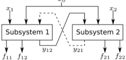
Subsystem 1 Subsystem 2
Figure 1: Representation of the interactions (y12andy21),
de-cision variables (x0,x1 andx2), and objectives (f11, f12, f21,
andf22) in the selected complex system.
(x0,x1,y21), and the two objective functionsf11(·)andf12(·)are to
be minimised. There is aK-dimensional vector of parameters de-noted byb=(b1, . . . ,bK)⊺, where each element is a weight, such thatbk≥0∀k=1, ...,K. The functiond(·)determines the Euclidean distance between the two points given as argument.
For Subsystem 2 the subproblem formulation is min f21(x2)=max ( max k=1, ...,Kckd(x2 ,ak),d(x2,y12) ) min f22(x2)=d(x0,x2),
such thatx0∈X0andx2∈X2
(2)
There are two decision variables,x0 andx2, wherex0 is shared,
implying that it exists in both subproblems. The local variablex2
takes values inX2 ⊆ R2. A solution to the above subproblem is
x2=(x0,x2,y12), and the two objective functions,f21(·)andf22(·),
are to be minimised. There is aK-dimensional vector of parameters denoted byc=(c1, . . . ,cK)⊺, where each element is a weight, such
thatck ≥0∀k=1, ...,K.
The interaction between the subsystems is captured by the link-ing functions,l1andl2, which leads to the following interacting
equations
y12=l1(x0,x1,y21):=x1
y21=l2(x0,x2,y12):=x2, (3)
It is then possible to say thaty12is an output of Subsystem 1
and an input for Subsystem 2; on the other hand,y21is an output
of Subsystem 2 and an input for Subsystem 1. A diagram that shows the inputs and outputs of the subproblems is shown in Figure 1.
In the following definitions, adapted from [5], we introduce the termssubsystemsolution andsystemsolution. The former is a so-lution obtained from the perspective of one subsystem, while the latter is a solution for the entire system, in that:
Definition 3.1. (Subsystem-feasible). A subsystem solution for Subsystem 1 isx1 = (x0,x1,y21)⊺, and it is called a
subsystem-feasiblesolution if (i)xi ∈Xi ⊆Rni for someni ∈Nandi=0,1, (ii)y21satisfies the interaction equationy21 = l2(x0,x2,y12), for
somex2 ∈ X2 ⊆Rn2andn2 ∈ N, wherey12 =l1(x0,x1,y21). A
similar definition applies to a subsystem solution for Subsystem 2 by swapping the indices of the variables.
Definition 3.2. (System-feasible). A system solution is denoted byx = (x0,x1,x2,y12,y21)⊺, and it is called asystem-feasible so-lution if (i)xi ∈ Xi ⊆ Rni for someni ∈ N andi = 0,1,2, and, (ii) bothy21andy12satisfy the interaction equationsy21 = l2(x0,x2,y12)andy12=l1(x0,x1,y21), respectively.
4
A NEW METHODOLOGY FOR
DISTRIBUTED MULTI-OBJECTIVE
OPTIMIZATION
A summary description of the steps in the proposed new methodol-ogy is shown below, whereNit er denotes the number of iterations. Assumptions are (i) that the original multi-objective optimization problem of the system has been decomposed into single- or multi-objective optimization subproblems and, (ii) for each pair of inter-acting subsystems, there is at least one shared decision variable.
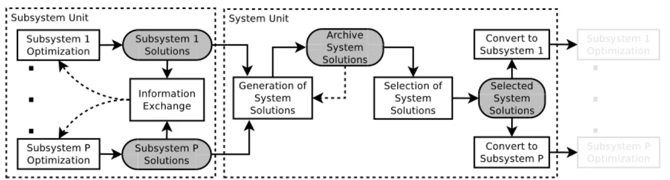
A diagram that illustrates the working of the methodology is shown in Figure 2. Note that there is a division between subsys-tem unitandsystem unit. In the former, the subsystems conduct their optimization tasks and exchange information via subsystem solutions. In the latter, the task is to aid the subsystems to generate subsystem-feasible solutions, eventually leading to system-feasible solutions. For this, the system unit is responsible for the genera-tion of system solugenera-tions, to identify system-feasible solugenera-tions and, to influence the optimization task in the subsystem unit.
Summary:Proposed methodology to support distributed col-laborative multi-objective optimization
Input: Lett=1, and specify a probability distribution for the linking variables.
1 Subsystem optimization: Run an optimizer until the budget is exhausted on the subproblem of each subsystem, with an initial randomly generated population. For each case, obtain a set of subsystem solutions with a population of sizeN(Section 4.1).
2 Information exchange: For each pair of interacting subsystems with their optimizer runs completed, update the prediction model of their linking variables. For this, the subsystems exchange information about their linking variables and shared decision variables (Section 4.2).
3 Generation of system solutions: Generate system solutions by combining
subsystem solutions from each subsystem and store them (both subsystem and system solutions) in an archive (Section 4.3).
4 Selection of system solutions: Select a subset of system solutions from the
archive, where the selection is based on a relaxed consistency constraint that becomes tighter with successive iterations (Section 4.4).
5 Convert system solutions to subsystem solutions: Extract the subsystem solutions from the selected system solutions. The obtained subsystem solutions replace a fraction of the initial randomly generated population in step 1 (Section 4.5).
6 Lett=t+1. Ift>Ni t e rthen stop, otherwise, go back to step 1.
An important feature of the methodology relates to its ability to support asynchronicity during the design process. Depending how the optimization task of the subsystems is coordinated, an approach can be categorised assynchronousorasynchronous. In a synchronous approach the subsystems conduct their optimiza-tion tasks in parallel and advance inlock-stepfashion. This means that at every step, the whole system has to wait until the most time-consuming optimization task completes. In an asynchronous approach, each design team works in parallel and information is communicated with other teams whenever it is generated. In Fig-ure 2, although all subsystems need to complete their optimizer runs for the system unit to generate system solutions, after the first iteration, the system unit operates asynchronously—a new set of system solutions is generated whenever at least one subsystem updates the generated solutions. This means that updated system solutions can be generated at a faster rate. Exploiting asynchronic-ity can be beneficial for systems with design teams that work at different rates, allowing the design process to move faster for more
GECCO ’18, July 15–19, 2018, Kyoto, Japan J. A. Duro et al.
Figure 2:Diagram of the proposed methodology. A grey box represents a population of solutions, and the other boxes are tasks. critical components of the system. The major steps of the
method-ology are described in more detail in the following sections.
4.1
Subsystem optimization
For the subsystems to be able to conduct their optimization tasks independently, the values of the linking variables have to be known before evaluating a solution. For instance, for Subsystem 1 to eval-uate a solution, it needs to know the value ofy21(see Section 3).
However, this value is provided by the linking functionl2, which is
only accessible to Subsystem 2. This means that without any infor-mation from Subsystem 2, Subsystem 1 needs to predict the value ofy21in order to evaluate a solution. Based on this, our approach
uses a model of the linking function that provides the values for the corresponding linking variable. This model is accessible to a subsystem, and allows, for instance, for Subsystem 1 to conduct an optimization task independently from Subsystem 2. The model used by the subsystems is as follows:
(1) First iteration: each linking variable is modelled as a random variable with a given probability distribution (e.g. a uniform probability distribution varying within the bounds of the linking variable). The assumption here is that the bounds of the linking variables are known. Although this allows the subsystem to explore the linking variable space, it may be the case that some regions of this space are infeasible (pos-sibly due to the constraints in the other subproblems), or simply because the sampled values of the chosen probabil-ity distribution are unrealistic or incorrect.
(2) Subsequent iterations: a supervised learning model learned (or constructed) by using the information shared between the subsystems. More details about the supervised learning model will be provided in Section 4.2.
Many multi-objective optimization algorithms rely on the con-cept of Pareto dominance for comparing solutions. This concon-cept is defined as follows.
Definition 4.1. (Classical Pareto Dominance). Let the decision vector of two solutions be given byx,x′ ∈ RD, whereDis the number of decision variables. Assuming minimisation,xis said to dominatex′(orxx′) iff: (i)fi(x)≤fi(x′)∀i=1, . . . ,M, where M is the number of objectives and (ii)∃j ∈ {1, . . . ,M}such that
fj(x)<fj(x′).
An optimization task running from the perspective of a sub-system that relies on Pareto dominance, will attempt to find the
non-dominated subsystem solutions that produce the best trade-offs amongst the objectives in the given subproblem, but it may fail to capture the trade-off solutions between the objectives of the different subproblems. This is because the subsystems do not have access to the objectives of each other’s subproblems, hence, subsys-tem solutions that appear dominated for a subproblem may actu-ally be non-dominated for the entire system problem. One way to capture such solutions is to rely on the Parameterized Pareto Dom-inance relation, previously proposed in [7], and defined as follows:
Definition 4.2. (Parameterized Pareto Dominance). Let the deci-sion vector of two solutions be given byx,x′ ∈RD. Let also the parameter vectors of the two solutions bep,p′∈RP, respectively, wherePis the number of parameters. Then,xis said to parametri-cally dominatex′, iffp
=p′andxx′.
Note that the parameter vectors in Definition 4.2 are analogous to the linking variables in a subproblem. The rationale for Defi-nition 4.2 lies in the argument that trade-off solutions across the system problem are likely to have different linking variable values. This is because the linking variables are an integral part of the ob-jective function’s domain, since the obob-jectives are often posed as a function of the linking variables. Retaining such solutions during an optimization task at subsystem level can be achieved by compar-ing the values of their linkcompar-ing variables, which is captured by the equalityp=p′in Definition 4.2. However, this equality is difficult to satisfy for real-valued linking variables, which can induce all so-lutions to become non-dominated. To overcome this, we propose to relax the requirement for equality by discretizing the linking space. This discretization involves partitioning the linking space into cells of the same size. Then, equality is deemed to be satisfied if the linking variable values of two solutions lie inside the same cell. The approach used for determining which cell a linking vari-able belongs to, is taken from [14] (Section IV-B). This requires the specification of the number of bins (nb) per dimension of the link-ing space. Note that, the largernbis, the larger the number of cells that partition the linking space.
4.2
Information exchange
After the subsystems have completed their own optimization tasks (as described in Section 4.1), an information exchange process takes place. This process is conducted on a peer-to-peer basis between any two interacting subsystems, and involves two subsystems ex-changing their subsystem solutions. The interchanged solutions
are employed to update the models of the linking functions, and subsequently, these models are used during the optimization pro-cess of the subsystems to predict the values of the linking variables. In case the models suffer from lack of accuracy (poor approxima-tion to the corresponding linking funcapproxima-tions), the obtained linking variable values might be incorrect or even unrealistic. As a conse-quence, subsystem solutions that contain such values: (i) cannot be subsystem-feasible (Definition 3.1) and, (ii) cannot be used to gen-erate a system-feasible solution (Definition 3.2). It is therefore im-portant for the subsystems to continuously exchange information about their linking variables as the iterations progress, allowing for the linking variable models to improve their accuracy.
To explain the information exchange process and model build-ing, consider the optimization model from Section 3. Subsystems 1 and 2 share a decision variablex0, and the interactions are
rep-resented by two linking variables, namelyy21andy12. The linking
variable,y12, is an output of Subsystem 1 and an input for
Sub-system 2. Hence, SubSub-system 1 is able to generate values fory12
since it has access to the linking function,l1, while Subsystem 2
needs to predict the values ofy12. Once Subsystem 1 completes
its own optimization task, the generated subsystem solutions are shared with Subsystem 2. The shared solutions, contain the values ofx0and correspondingy12, and represent the set of trade-offs
pre-ferred by Subsystem 1. These values are then used by Subsystem 2 to construct a supervised learning model wherex0andy12are
used as training data. This means thatx0is treated as the model
input, whiley12 is the output (or target). Given this, we seek to
learn a function approximation of the linking functionl1, with the
following formf1(x0) =y12. The same procedure is followed by
Subsystem 1 for constructing a model to approximate the linking functionl2, that isf2(x0) =y21, which allows for predictions to
be made abouty21. For constructing either models, a supervised
learning algorithm can be used.
The constructed models are used by the Subsystems during their own optimization task to predict the values of the linking variables. This means that each time a new solution is to be evaluated, first, the value of the shared variable (x0) is chosen by the optimizer, and
then,f1(x0)(orf2(x0)), is evaluated with the given,x0, and the
pre-dicted value of the linking variable is obtained. Let the prediction value of the linking variable be denoted by ˜y12for Subsystem 2 and
˜
y21for Subsystem 1.
4.3
Generation of system solutions
The generation of a system solution involves combining subsystem solutions, and the approach used is based on the Stackelberg com-petition or follower model [13]. This implies that a leader-follower relationship is defined between the subsystems, and this relationship is used to determine which subsystem solutions are chosen for setting the values of the system solution. A system so-lution generated in this way can incur in aconsistency error, which depends on the difference between the linking variable values of the subsystem solutions. The number of system solutions to be gen-erated is a user-defined parameter, and we suggest that it be set to N, the size of the initial population.
An archive is used to keep track of all generated system solu-tions, including the subsystem solutions used to generate them.
Given that the number of solutions in the archive increases after each iteration, it is proposed to use a threshold that sets an upper bound on the number of solutions allowed in the archive, and let it be ˙Nmax. Thus, when the number of solutions in the archive ex-ceeds ˙Nmax, a selection approach described in Section 4.4 is used to reduce the number of solutions to exactly ˙Nmax.
To generate a system solution, it is first required to draw a ran-dom sequence that defines an order between the subsystems. This allows for different relationships between the subsystems to be ex-plored. For a single system solution, let this sequence be denoted byr ={r1, . . . ,rS}whereri ∈ {1, . . . ,S},ri ,rj∀i,j=1...S,i,j, and Sis the number of subsystems. The following two steps lead to the generation of a single system solution. The first applies a criterion to select the subsystem solutions (one from each subsystem), while the second generates a system solution by combining the chosen subsystem solutions. The following two sections describe the pro-cedure adopted by each step.
4.3.1 Selection of subsystem solutions. The subsystem solutions can be selected from:
(1) The populations of subsystem solutions obtained by each optimizer: LetP = {P1, . . . ,PS} be a set that stores the populations from all subsystems, andPi ={xi1, . . . ,xi N}, wherexi jis a subsystem solution for theith subsystem in thejth position of the populationPi.
(2) An archive: let it be given byA = {A1, . . . ,AS}, where Ai = {x˙i1, . . . ,x˙iN˙}, and ˙xi j is a subsystem solution for theith subsystem in thejth position of the archive. Let ˙N to be the current number of solutions in the archive where 0 ≤ N˙ ≤ Nmax˙ . For each set of subsystem solutions at any position in the archive (say thejth position), that is {x˙1j, . . . ,x˙S j}, the archive also keeps track of the correspond-ing system solution. Durcorrespond-ing the first iteration, the subsys-tem solutions are only selected fromPsince, initially, the archive is empty.
The selected subsystem solutions are stored in a set, given by
s={s1, . . . ,sS}, wheresi is the subsystem solution of theith sub-system. Different strategies can be employed to select the subsys-tem solutions. A simple strategy is to select the solutions randomly fromP. First, letU(N)denote a uniform distribution on{1, . . . ,N}. Then, the solution for theith subsystem is
si =xi j,such thatj∼U(N). (4)
Equation 4 is used to select the solutions inswhich correspond to “leader” subsystems, as opposed to “follower” subsystems. A subsystem is considered to be a leader if it is the first in the se-quencer, amongst the subsystems that share the same decision variable(s), while the others are the followers. This means that each follower subsystem can use a leader subsystem as a reference for se-lecting its own solutions. Thus, the solutions inscorresponding to leader subsystems are selected first, and afterwards, the selection takes place for follower subsystems. Given this, the strategy for se-lecting solutions inswhich correspond to follower subsystems is as follows. First, let theith subsystem be any follower subsystem, and let thelth subsystem be the corresponding leader. Then, the
GECCO ’18, July 15–19, 2018, Kyoto, Japan J. A. Duro et al.
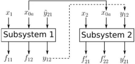
Subsystem 1 Subsystem 2
Figure 3: Generation of a system solution, where Subsystem 1 is the leader and Subsystem 2 is the follower.
solution for theith subsystem is
si = ( xi j,ifh xi j,sl ≤h(x˙ik,sl) ˙ xik,otherwise such that j= argmin j∈ {1, ...,N} hxi j,sl andk= argmin k∈ {1, ...,N˙} h(x˙ik,sl) (5)
where the functionh(·)uses the Euclidean distance to calculate the distance between the shared variable values of the two solu-tions given as input. Equation 5 aims to reduce the consistency error of the system solution that is to be generated by the chosen subsystem solutions ins. Given that this error increases with an increment in the difference between the values of the linking vari-ables, a way to reduce it, is to select the subsystem solutions such that the distance between their linking variables values is as small as possible. For this, we use the shared variables, since the model used to predict the values of the linking variables is posed as a func-tion of the shared variables. Hence, the closer the shared variable values are, the closer the linking variable values are likely to be, effectively reducing the consistency error of the system solution.
Note that, for the model of Section 3 there are only two subsys-tems in the problem, implying that only two sequences forr are possible, that is, eitherr={1,2}orr={2,1}. For the former, Sub-system 1 is chosen as the leader while SubSub-system 2 is the follower, and subsystem solutions from Subsystem 1 and 2 are selected by Equations 4 and 5, respectively. The contrary is true for the latter.
4.3.2 Generation of a system solution.A system solution is now generated by using the subsystem solutions insand the sequence inr. Due to space limitations, we describe this procedure only with respect to the model of Section 3. However, this procedure can be generalised for problems with a greater number of subsystems and different characteristics.
Consider a subsystem solution for Subsystem 1 denoted byx1=
(x0a,x1,y˜21)with output(f11,f12,y12). Similarly for Subsystem 2,
letx2 = (x0b,x2,y˜12)be a subsystem solution and the output is
(f21,f22,y21). Note thatx0a andx0b represent the same shared variable, but their values can be different. The procedure is now described only for the sequencer={1,2}, and it is also illustrated in Figure 3. The steps are as follows:
(1) create a solution for Subsystem 2 by selecting the shared variable and linking variable fromx1, and the local variable
fromx2, leading tox2′=(x0a,x2,y12).
(2) conduct an evaluation of Subsystem 2 (Equation 2) withx2′
and obtain(f21′,f22′,y21′ ).
(3) create a system solution that is comprised of the shared, lo-cal and linking variables fromx1, and also the local variable
fromx2, leading tox=(x0a,x1,x2,y12,y˜21). The output of
the system solution is comprised of the output fromx1, the
output fromx2′, which leads to(f11,f12,f21′,f22′,y12,y′21).
(4) the consistency error of the system solution is the difference between (i) the predicted value of linking variable byx1, i.e.
˜
y21and, (ii) the new linking variable value obtained by the
evaluation in step 2, i.e.y′21. This is given by||y˜21−y′21||.
4.4
Selection of system solutions
A selection procedure is applied to the system solutions in the archive and a subset of system solutions is chosen. The procedure is based on the selection used by NSGA-II [2] to select an elite population. This consists of a constraint handling approach, non-dominated sorting and crowding distance. The first requires a con-straint function to be specified, the second ensures that only solu-tions with improved convergence are selected, and the third is used to guarantee a good distribution across the Pareto-optimal set. It is suggested that the size of the selected subset is set to be one-half of the population size (N). This means that half of the population of each subsystem in the next iteration is determined by the system solutions, while the other half is generated randomly.
The constraint function used by the selection approach is now described. One possible constraint function is to simply use the consistency error of the system solutions. Then, if this error is greater than zero, the solution is considered infeasible, otherwise it is feasible. However, this error is never likely to be exactly zero, since the computation of this error may involve determining the difference between real-valued numbers. Therefore, this means in practice that all system solutions may be infeasible and the solu-tions are “always” only ranked based on their infeasibility, rather than non-dominated sorting and crowding distance. To avoid this, we propose a dynamic threshold that depends on the current iter-ation number. For this, consider the setx ={1, . . . ,Nit er}. Then, the threshold value at theith iteration is given by the following regression function δi = cmax,i=1, cmax−cmax−cmi n Ni t e r1/p x 1/p i ,i=2, . . . ,Nit er, (6) wherecmaxandcminare the maximum and minimum consistency errors, whilepis the power (or inclination) of the regression. It is suggested thatcmin = ϵ whereϵis set to a very small number (say 1×10⁻⁶), whilecmaxandpare user-defined parameters. The
threshold value obtained by the function in Equation 6 decreases fromcmax tocmin, over the successive iterations. Furthermore, a system solution(x0,x1,x2,y12,y21)⊺is considered to be system-feasible at theith iteration if its consistency error (let it be denoted byxe) is less than or equal toδi. This is expressed mathematically by the expression
дi(x0,x1,x2,y12,y21)≡xe ≤δi. (7) The constraint function in Equation 6 ensures that not all sys-tem solutions are considered as infeasible in the early stages of the distributed optimization run. This allows other operators (conver-gence and diversity) to participate in the selection process. As the
threshold value approachescmin, the pressure to generate system solutions with a lower consistency error increases, leading to a set of solutions that are consistent, and with a good convergence to and diversity across the Pareto-optimal front.
4.5
Convert system solutions to subsystem
solutions
Individual subsystem solutions are now extracted from the selected system solutions. This procedure is described with respect to the model from Section 3. For this, let a system solution be denoted by
(x0,x1,x2,y12,y21)and the output is(f11,f12,f21,f22,y12′ ,y21′ ). The
extracted subsystem solution for Subsystem 1 is(x0,x1,y21)and
the output is(f11,f12,y12′ ). In addition, the subsystem solution for
Subsystem 2 is(x0,x2,y12)and the output is(f21,f22,y′21).
The subsystem solutions obtained by this procedure are used to influence the optimization task of the subsystems, during the next iteration. For this, these solutions replace a fraction of the initial (randomly) generated solutions. Given that the suggested size of the selected solution subset is one-half of the population size (N) (as mentioned in Section 4.4), it implies that half of the initial population corresponds to the selected subsystem solutions, and the other half are generated randomly.
5
DEMONSTRATION OF THE NEW
METHODOLOGY
5.1
Experimental setup
The general parameters are as follows. The budget allocated for the optimization run is 100000 system solution evaluations, with subsystem evaluations counting partially toward the budget. The available budget is distributed amongst the number of iterations, which is set toNit er =50. This implies that the number of func-tion evaluafunc-tions per iterafunc-tion is 100000/50= 2000. This number needs to be divided between the optimization in the subsystem unit and the generation of system solutions. First, knowing that the population size for each subsystem is set toN = 120, and that only half of the objectives are evaluated for each generated system solution, the number of function evaluations for the gen-eration of system solutions isN/2 = 60. Second, the number of function evaluations per subsystem is then set to the remainder, that is,(2000−60)=1940.
The specific parameters for each task of the proposed method-ology are as follows:
(1) For subsystem optimization (Section 4.1): NSGA-II is cho-sen as the underlying optimizer for each subsystem, where the probability of crossover and mutation are 0.9 and 0.1, re-spectively. For partitioning the linking variable space, the number of bins (nb) is set to 20.
(2) For information exchange (Section 4.2). Anartificial neural network(ANN)1is chosen as the supervised learning model. The chosen parameters correspond to those suggested by the author of the library. These are as follows, (i) the number of hidden layers is set to 1, (ii) the number of hidden nodes in the hidden layer is set to 13, (iii) the Sigmoid symmetric 1Thefast artificial neural network(FANN) library is used and a description is found
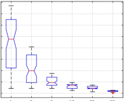
in http://fann.sourceforge.net/fann_en.pdf . 1 2 5 10 20 50 Iterations 0 0.1 0.2 0.3 0.4 0.5 0.6 0.7 0.8 Consistency error
Figure 4: Consistency error of the selected system solutions along the iterations of the distributed approach, for one run.
function is used as the hidden and output functions and, (iv) the maximum number of epochs is set to 200.
(3) For generation of system solutions (Section 4.3): The maxi-mum number of solutions in the archive is ˙Nmax =2000. (4) For selection of system solutions (Section 4.4):cmax is set
to the lowest consistency error obtained by at least 5% of the system solutions in the first iteration of the distributed approach, and the regression powerpis set to 3.
A comparative analysis is conducted between the proposed ap-proach and a monolithic apap-proach based on the AAO problem. NSGA-II is the optimizer for the monolithic approach, set with the same parameters mentioned above. Both approaches are applied to the model from Section 3, and the parameters of the model are:
A= 00..873801 00..291801 00..546622 00..165142 00..844944 !⊺ , b=(0.020,0.059,0.087,0.419,0.415)⊺, c=(0.148,0.262,0.132,0.223,0.235)⊺. (8)
For comparing the results between the two approaches, the hy-pervolume indicator is used. The computation uses a dimension-sweep algorithm, taken from [3]. To select the reference point re-quired to measure the hypervolume, the non-dominated solutions obtained at the end of each iteration are used. To ensure that any population of solutions can be compared, the reference point is set to the maximum objective values obtained by all iterations across all simulations conducted.
5.2
Experimental results
This section demonstrates the application of the proposed method-ology to the optimization model described in Section 3.
The first analysis is conducted based on one single simulation run. In Figure 4 the consistency error of the system solutions which have been selected by the system unit is shown. Note that thex -axis scale is not linear, and that in just 10 iterations the consistency error has dropped from a maximum of 0.7 to a value less than 0.1. This highlights the effectiveness of the proposed methodology in reducing the consistency error of the system solutions.
We now conduct a comparative analysis between the distributed approach and the monolithic approach. Both the distributed ap-proach and the monolithic apap-proach are run for the same number
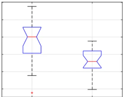
GECCO ’18, July 15–19, 2018, Kyoto, Japan J. A. Duro et al. Monolithic Distributed 2.35 2.4 2.45 2.5 2.55 2.6 Hypervolume
Figure 5: Comparative analysis between monolithic and dis-tributed approach, each boxplot corresponds to 20 runs.
of function evaluations, and a total of 20 runs are conducted. For the distributed approach, the hypervolume metric is applied to the objective vectors of the system solutions after being evaluated by the monolithic problem formulation. This is because the objective values of the system solutions that have been evaluated by the dis-tributed approach, can differ from those values that are obtained by the monolithic problem due to the consistency error.
The hypervolume obtained for the final population by each ap-proach is shown in Figure 5. Note that, as expected, the mono-lithic approach outperforms the distributed approach, where the obtained mean for the monolithic approach is 2.48 and the obtained mean for the distributed approach is 2.43. Therelative percentage difference2between the two means is only 2.31%, which highlights that the performance of the distributed approach is comparable to the monolithic one in this particular case study.
6
CONCLUSION
This paper has proposed a new methodology for distributed multi-objective optimization of complex systems with interacting subsys-tems. This methodology adopts a distributed approach where the subproblems do not have access to each other’s design problems, and only limited information is shared between them. A system unit is used to aid the subsystems to generate subsystem-feasible solutions, eventually leading to system-feasible solutions.
At the subsystem level, the optimization task for each subprob-lem uses the parameterized dominance relation, which has been adapted to handle real-valued linking variables. For handling the interactions, the subsystems exchange information about their own optimal solutions on a peer-to-peer basis. The received informa-tion is used to construct a representative model of the linking vari-ables by employing a supervised learning algorithm, which allows the subsystems to predict each other’s responses. At the system level, a leader–follower based approach is employed for the gener-ation of system solutions. The best system solutions are chosen to influence the optimization at subsystem level.
The performance of the new methodology has been studied on a complex system with two interacting subsystems. A comparative
2Therelative percentage differencebetween two values (sayv
1andv2) is given by
|v1−v2|/max(|v1|,|v2|)×100.
analysis of the proposed distributed approachvsa monolithic ap-proach has been conducted. The obtained results show that the pro-posed approach is not outperformed by the monolithic approach. The significance of the method described is that it effectively ad-dresses the need to design complex systems, where subsystems are designed by teams adopting a collaborative asynchronous strategy.
7
ACKNOWLEDGMENTS
This work was supported by Jaguar Land Rover and the UK-EPSRC grant EP/L025760/1 as part of the jointly funded Programme for Simulation Innovation. JAD is the primary author and researcher; YY contributed to the development of the software architecture that supported our work; RCP and PJF provided guidance and con-tributed to the development of the methodology and paper.
REFERENCES
[1] B. Dandurand and M. M. Wiecek. 2015. Distributed Computation of Pareto Sets.
SIAM Journal on Optimization25, 2 (June 2015), 1083–1109.
[2] K. Deb, A. Pratap, S. Agarwal, and T. Meyarivan. 2002. A Fast Elitist Multi-Objective Genetic Algorithm: NSGA-II.IEEE Transactions on Evolutionary Com-putation6, 2 (April 2002), 182–197.
[3] C. M. Fonseca, L. Paquete, and M. López-Ibáñez. 2006. An Improved Dimension-Sweep Algorithm for the Hypervolume Indicator. InInternational Conference on Evolutionary Computation. IEEE, Vancouver, CA, 1157–1163.
[4] C. Huang, J. Galuski, and C. L. Bloebaum. 2007. Multi-Objective Pareto Concur-rent Subspace Optimization for Multidisciplinary Design. AIAA Journal45, 8 (August 2007), 1894–1906.
[5] K. Klamroth, S. Mostaghim, B. Naujoks, S. Poles, R. Purshouse, G. Rudolph, S. Ruzika, S. Sayin, M. M. Wiecek, and X. Yao. 2017. Multiobjective optimization for interwoven systems.Journal of Multi-Criteria Decision Analysis24, 1-2 (February 2017), 71–81.
[6] W. Maier M. 1999. Architecting principles for systems-of-systems.Systems En-gineering1, 4 (February 1999), 267–284.
[7] R. J. Malak and C. J. J. Paredis. 2010. Using Parameterized Pareto Sets to Model Design Concepts.Journal of Mechanical Design132, 4 (April 2010), 1–11. [8] J. R. R. A. Martins and A. B. Lambe. 2013. Multidisciplinary design optimization:
a survey of architectures.AIAA journal51, 9 (July 2013), 2049–2075. [9] C.D. McAllister and T.W. Simpson. 2003. Multidisciplinary robust design
Opti-mization of an internal combustion engine.Journal of mechanical design125, 1 (March 2003), 124–130.
[10] C.D. McAllister, T.W. Simpson, K. Hacker, K. Lewis, and A. Messac. 2005. Integrat-ing linear physical programmIntegrat-ing within collaborative optimization for multiob-jective multidisciplinary design optimization. Structural and Multidisciplinary Optimization29, 3 (October 2005), 178–189.
[11] S. Parasha and C. Bloebaum. 2006. Multi-Objective Genetic Algorithm Concur-rent Subspace Optimization (MOGACSSO) for Multidisciplinary Design. In47th AIAA/ASME/ASCE/AHS/ASC Structures, Structural Dynamics, and Materials Con-ference, Vol. 8. AIAA, Newport, Rhode Island, 5523–5533.
[12] S. Rabeau, P. Dépincé, and F. Bennis. 2007. Collaborative optimization of com-plex systems: a multidisciplinary approach.International Journal on Interactive Design and Manufacturing1, 4 (November 2007), 209–218.
[13] J. R. J. Rao, K. Badhrinathy, R. Pakalay, and F. Mistree. 1997. A Study of Opti-mal Design Under Conflict Using Models of Multi-Player Games. Engineering Optimization28, 1-2 (October 1997), 63–94.
[14] D. K. Saxena, A. Sinha, J. A. Duro, and Q. Zhang. 2016. Entropy-Based Termi-nation Criterion for Multiobjective Evolutionary Algorithms.IEEE Transactions on Evolutionary Computation20, 4 (August 2016), 485–498.
[15] R. V. Tappeta and J. E. Renaud. 1997. Multiobjective Collaborative Optimization.