A Study of Rating Curve and Flood Routing using Numerical Method

(1)

A STUDY OF RATING CURVE &

FLOOD ROUTING USING

NUMERICAL METHODS

Prateek Kumar Singh

Department of Civil Engineering

(2)

A STUDY OF RATING CURVE AND

FLOOD ROUTING USING

NUMERICAL METHOD

A dissertation submitted to the National Institute of Technology, Rourkela

in partial fulfilment of the requirements of the degree of

Master in Technology

in

Civil Engineering

By

Prateek Kumar Singh

(Roll Number:

215CE4286

)

Under the supervision of

Prof. K. K. Khatua

June, 2017

Department of Civil Engineering

(3)

Department of Civil Engineering

National Institute of Technology, Rourkela

June 02, 2017

Certificate of Examination

Roll Number: 215CE4286 Name: Prateek Kumar Singh

Title of Dissertation: A STUDY OF RATING CURVE AND FLOOD ROUTING USING NUMERICAL METHOD

The undersigned, after examining the thesis mentioned above and the official record book (s) of the student, hereby state my approval of the dissertation submitted in partial fulfillment of the requirement of the degree of Masters in Technology in Civil Engineering at National Institute of Technology, Rourkela. We are satisfied with the volume, quality, correctness, and originality of the work.

(External Examiner)

Date:

(4)

Department of Civil Engineering

National Institute of Technology, Rourkela

K. K. Khatua

Professor June 02, 2017

Supervisor’s Certificate

This is to certify that the work presented in this dissertation entitled “A Study of Rating curve and Flood Routing Using Numerical method” by “Prateek Kumar Singh”, Roll Number: 215CE4286 is a record of original research carried out by him under my supervision and guidance in partial fulfillment of the requirements of the degree of Master in Technology in Civil Engineering. Neither this dissertation nor any part of it has been submitted for any degree or diploma to any institute or university in India or abroad.

K. K. Khatua

(5)

DEDICATED TO

MY Nation

(6)

Declaration of Originality

I am Prateek Kumar Singh bears a Roll Number: 215CE4286 want to affirm that this dissertation entitled “A Study of Rating curve and Flood Routing Using Numerical method” is an original work carried out for the partial fulfillment of Masters’ degree in NIT Rourkela. It does not comprise any material previously published or written by another person, nor any material presented for the award of any degree or diploma of NIT Rourkela or any other institution. Any contribution made to this research by others, with whom I have worked at NIT Rourkela or elsewhere, is explicitly acknowledged in the dissertation. Also, the works of other authors cited in this dissertation have been duly acknowledged under the section “Bibliography”.

I am fully aware that in case of my non-compliance detected in the future, the Senate of NIT Rourkela may withdraw the degree awarded to me based on the present dissertation.

June 02, 2017

Prateek Kumar Singh NIT Rourkela

(7)

Acknowledgment

I would like to thank the Civil Engineering Department of National Institute of Technology, Rourkela for providing me the necessary resources and funding for the completion of my thesis and project work for the duration of this Masters’ work.

There are many people that I would like to thank, both academically and socially, for inspiring my life over past two years. First, I would like to express my gratefulness to my supervisor, Prof. Kishanjeet Kumar Khatua for his constant guidance, criticism and enthusiasm that allowed all of the work to be possible. Without his great support and encouragement, it would have been impossible to work constantly and efficiently. I would also thank Prof. Sanat Nalini Sahoo, Prof. Awadhesh Kumar and Prof. Kanhu Charan Patra for sharing with me their wealth of knowledge. Their helpful discussion in person and their belief, which made me more serious and sincere for my work, I give my sincere and heartfelt thanks.

I would like to express special thanks to all my colleagues of hydraulic lab specially Arpan Pradhan, Bandita Naik, Saine Sikta Das, Sumit Baneerjee, Arun Kumar, Sarjati Sahoo and many others for their constant contribution towards my work as well as their care and patience to handle my mood swings through tough times.

Beside work partner there is always a need of a fun partner with whom we energize and refresh our mind to have a great time while working. Many thanks to my fun group Sovan Sankalp Prince Raj, Sateesh Yadav, Pushpendra Kumar, K. Prakash, Kamli Kumar, Mishra, Tiwari, Bishu, Alok and many more without whom memories would have been less colorful. Finally yet importantly, I would like to thank my parents Awadhesh Kumar Singh and Damyanti Singh for their love, care, patience, encouragement and belief in me.

June 02, 2017

Prateek Kumar Singh

(8)

Abstract

The stage discharge curve, depth-averaged velocity and boundary shear stress distributions are essentially determined for the flood extenuation scheme. The difficulties aroused in prediction of these parameters are usually due to the 3D nature of the fluid flow in open channel. The current study represents different analytical model for velocity distribution, boundary shear stress and stage-discharge curves and their application to the trapezoidal compound channel. The analytical solution to the depth-integrated Navier-Stokes equation is used for the same and their results are validated using experimental data. These parameters are not easy to predict because of the three-dimensional characteristics of the flow field. The model proposed by Shiono and Knight (1988, 1991) is compared with those by Ervine et al. (2000), Kordi et al. (2015) and K-ε model (ANSYS) through numerical modelling. This test shows that secondary flow parameter plays a vital role and its significance proliferates near side slope where momentum transfer from the main channel to flood plain is observed. The contrast in the results are shown with the help of lateral variation in percentage error.

The flood routing is an important technique to determine the flood peak attenuation and the duration of the high water levels through channel routing. Beside stage-discharge curve, hydrographs also plays a vital role in flood prediction and forecasting. The present study shows the application of hydrological methods for channel routing, the constant coefficient Muskingum-Cunge (MC) methods on the River Brosna, Co. Offaly in Ireland. The results obtained are validated by two software packages MIKE 11 and HEC-RAS beside that the method ensuring the mass balance of the model is tested in terms of water storage. The results of all the tests are plotted and verified with respect to the mass conservation criteria. Data sets of the River Brosna, Co. Offaly in Ireland is taken from the Elbashir (2011) for the November 1994 flood event.

Keywords: Shiono Knight Method, Extended SKM, Secondary parameters, compound channel, Open channel, Muskingum-Cunge, Mass conservation

(9)

List of Figures

1 Shear stress distribution on the boundary of a trapezoidal channel ... 20

2 Stage Discharge Curve for B/b 4.2 Flood channel facility phase A series 02 ... 22

3 Schematic representation of controls range in rating curve ... 23

4 Hydrograph of inflow and outflow flood event 1994 River Brosna, Ireland ... 24

5 Hydrograph elements ... ..24

6 Flood routing hydrograph for natural river Brosna, Offaly Ireland Elbashir (2011)………...…...26

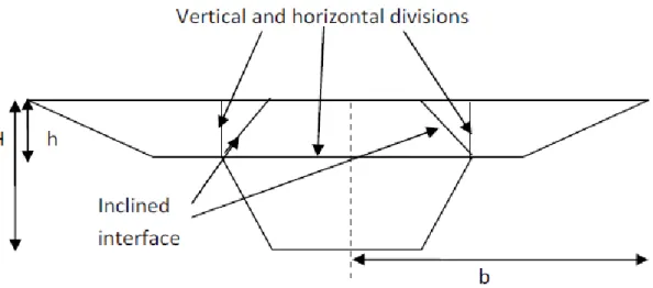
7 Secondary current vectors in trapezoidal smooth channels (Tominaga et al.1989).51 8 Possible division lines (both horizontal, vertical and inclined) for divided channel method (Chlebeck 2009) ... 56

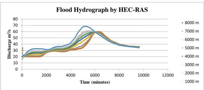
9 Flood event Nov-Dec 1994 Brosna River using HEC-RAS ... 74

10 Six (6) Point Abbott-Ionesco schemes and implicit scheme used in Mike 11 ... 75

11 Discretization of river branch in the Mike 11 hydrodynamic model ... 76

12 Discretization of cross section of river in the Mike 11 and illustration of both the lateral profile and the cross-section for the Brosna Offaly river reach ... 77

13 Flood event Nov-Dec 1994 Brosna River using MIKE 11 ... 81

14 Symmetric compound channel with side slope s=1 ... 82

15 Cross section of the river reach …….. ... 83

16 Ud (y)) distribution for experiment FCF phase A series 02 and 03 (a) to (c) B/b 2.2 & (d) to (f) B/b 4.2 for various model with and without inclusion of secondary flow in SKM ... 88

17 τb (y) distribution for experiment FCF phase A series 02 and 03 (a) to (c) B/b 2.2 & (d) to (f) B/b 4.2for various model with and without inclusion of secondary flow in SKM ... … 91

18 Stage discharge curve for FCF phase A series 02 and 03 ... ………92

19 Flood hydrograph at eight sub-reaches of river Brosna for flood event 1994 ... 95

20 Flood hydrograph at eight sub-reaches for river Brosna for flood event 1994 using Muskingum-Cunge, HEC-RAS and MIKE 11 ... 99

(14)

22 A comparisons among the predicted relative error values by the different models ... 104

23 A comparisons among the predicted values and the measured value of depth-averaged velocity by the different models ... …….106

(15)

List of Tables

1 Factors for computing wave speed from average velocity (US Army Corps of Engineers, 2008 ... 28

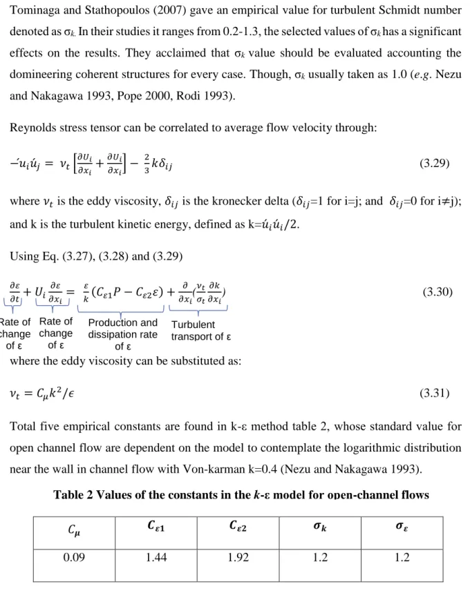
2 Values of the constants in the k-ε model for open-channel flows ... 63

3 River Brosna reach characteristics ... 83

4 Hydraulic parameters of the cross sectional area of river Brosna for flood event 1994 ... 93

5 Coefficients of routing calculation for river Brosna for flood event 1994 ... 94

6 Conservation of mass consideration EVOL% of every sub-reach of river Brosna flood event 1994 ... 107

(16)

Nomenclature

v̅ Time-averaged spanwise velocity

w̅ Time-averaged vertical velocity

𝑢̅ Time-averaged streamwise velocity

∆𝑡 Computational interval

∆𝑥 Spatial Weightage factor A Area of the compound section b Bottom width of main channel B Over all width of compound channel

C Volume fraction

C Courant number

Cd Dynamic celerity Co, C1, C2 Routing Coefficients

D Cell Reynold’s number

Dm Hydraulic depth

f Darcy-Weisbach Friction factor Fr Froude’s number of the flow g Acceleration due to gravity g Gravitational acceleration

h Height of main channel up to floodplain bed H Total depth of flow in compound channel

H Water depth

hv Velocity head

i Stands for local values in the ith cell or node I turbulence intensity

k Turbulence kinetic energy

K Ervine’s coefficient for K-method

L Non prismatic length of converging compound channel

L Reach length

n Manning’s roughness factor

(17)

Q Discharge

q The unit flow rate Qactual Actual discharge Qo References discharge

R Hydraulic mean radius of the channel cross section (A/P) Re Reynolds number of the flow

S Valley slope S Storage Sf Friction slope So Bed slope t Time T Top width

U Instantaneous streamwise velocity U Shear velocity

u’ Streamwise fluctuation velocity Ud Depth-averaged streamwise velocity V Instantaneous spanwise velocity v’ Spanwise fluctuation velocity W Instantaneous vertical velocity w’ Vertical fluctuation velocity

x Cartesian coordinate in the streamwise direction y Cartesian coordinate in the spanwise direction z Cartesian coordinate in the vertical direction

β Ratio of kinematic celerity to the average longitudinal velocity Γ Secondary flow term

ϵ Rate of dissipation of turbulent kinetic energy k ϵyx Kinematic eddy viscosity

λ The dimensionless eddy viscosity λ Eddy viscosity coefficient

μ Dynamic viscosity of water ν Kinematic viscosity of water ρ Density of flowing liquid σk Turbulent Schmidt number τ Point boundary shear stress

(18)

τd Bed shear stress lateral distribution

τxx, τxy, τyx, and τyy The depth integrated Reynolds stresses in appropriate directions Г1 Helical secondary current

Г2 Transverse convection term є The eddy viscosity

(19)

Chapter 1 Introduction

Chapter 1

INTRODUCTION

1.1 General

Estimation of the flow discharge with respect to the stage and the time is one of the main parameters in the flood management projects. The insurance companies have also acknowledged the importance of the prediction of the flow discharge. Estimation of flow discharge leads to evaluate the flow depth in streams is necessary to estimate the risk of insurance of projects located on the floodplains. The stage-discharge curve is very crucial for the prediction, computation and the forecast of flood in a natural river system. When a flood occurs, the flow depth increases arbitrarily which in turn causes overbank flow. The overbank flow is usually very different from that of the inbank or single channel flow. The characteristic of the floodplain in the overbank flow plays a vital role, whereas the difference in the flow of water in the floodplain and the main channel generates strong lateral shear layer and large-scale turbulence (Sellin 1964; Perkins 1970; Wormleaton and Merrett 1990; Ackers 1992; Tominaga and Nezu 1991; Bousmar and Zech 1999). The occurrence of large eddies due to the vertical vortices and helical secondary flows is most substantial feature in the longitudinal direction (Rodi 1980). Ignorance of such coherent structure may always lead to the error, in prediction of the velocity and the boundary shear stress distribution.

Velocity distribution and boundary shear stress distribution is the key feature for the prediction of the water surface profile, compound open channel design, and sediment and pollutant transport in the overbank flow. Many modelling techniques are presented in the past literature for the prediction of the velocity distribution, such as single channel method, divided channel method (Lotter 1933; Te Chow 1959), coherence method (Ackers 1992, 1993; Lambert and Sellin 1996), weighted divided channel method (Lambert and Myers 1998), exchange discharge model (Bousmar and Zech 1999), lateral discharge method using Reynolds averaged Navier-Stokes equation (RANSE) (Shion and Knight 1988,1991; Ervine et al. 2000) and so on. The prediction of the boundary shear stress distribution in a gravity flow channel is very significant because this is that parameter which influence flow

(20)

structures in the channel, the conveyance capacity and the transportation of the sediments in the channel (Knight 1981; Graf 1991; Knight and Sterling 2000; Sterling et al. 2008).

On the other hand, climate change is another factor affecting the hydrological processes, which has profoundly changed the approach of the engineers in the past few decades. Further, engineers and hydrologist face problems related to the hydrology of the ungauged basin because of the unavailability of the morphological, hydrological and hydrometric data for the basins, especially in the developing and under-developed countries (Perumal and Price 2013). These problems of hydrological non-stationarity and ungauged basins necessitates decision making based on the hydrological models that are numerically governed solution for the basic equation of flow which are integral to these hydrological component processes.

Flood routing is another approach for the flood planning and management. Study of flood wave movement in the channel and Natural River is one of the most important hydrological investigation using the basic governing equation of flow. Many studies have been performed which showed the consistency of such hydrological routing methods. Ponce (1981) and Merkel (2002) showed the consistency of the MC method (constant parameter) and developed the outflow hydrograph using different step and time size interval. Reid (2009) suggested more research on the short reaches and small drainage area, which are the conventional cases experienced while the application of the hydrological channel routing method.

The difficulties in dealing with a small channel are the milder slope, which lack good quality flow data, which are most significant for modelling and comparison purpose. These aspects influence the precision of the two approaches and introduce sources of error in the assessment process.

1.2 Velocity distribution

In a circular duct, the profile is considered parabolic for laminar flow conditions. However, the velocity profile in open channel flow is usually turbulent and fluctuates because of friction generated at the bottom and sidewalls. The velocity increases as we move away from the boundaries in either lateral or longitudinal direction, or it would indicate that the maximum velocity would occur at the midway from both side boundaries and over the free

(21)

not make the ideal condition possible for the location of maximum velocity and hence the velocity dip near surface comes into the picture. In case of rectangular channel, the point of maximum velocity on a vertical line would occur close to the water surface if the vertical line is taken at the centre. As we move closer to the banks, the point of maximum velocity will tend to move downward. In contrast to narrow rectangular channel if wide rectangle channels are considered the maximum velocity will occur closer to the water surface in wide channels.

Some of the important observations regarding the velocity distribution in open channel flow are as follows:

1. The velocity at the depth of 0.6 times the total flow depth from the water surface level is considered as the depth average velocity in general. This has important application since discharge is sometimes calculated from the contour diagram through area-velocity method. Rather calculating velocity at every point and then averaging it to obtain the average velocity, it would be more convenient to measure the average velocity at a particular point which is 0.6y below the water surface, and where y is the flow depth at that vertical line.

2. An even more accurate method to estimate the average velocity is to measure the point velocity at two different location i.e. 0.2y and 0.8y from the water surface. Note that these locations are nearly identical with the location of Gauss points, which are numerically integrate an arbitrary function with best possible accuracy using two points the values of Gauss points are 0.5[1± (1/√3 )], i.e. 0.79 and 0.21 of the flow depth.

3. The magnitude of the surface velocity is almost 5-25% more than that of the average velocity. The channel dimension and flow characteristics play significant role in determining the exact ratio of the surface velocity and average velocity. This ratio remains more or less constant for a given channel under comparable flow conditions.

1.3 Boundary shear stress

The average boundary shear stress on the channel has been shown (through a balance of driving and resisting forces under uniform flow conditions) to be equal to ρgRS where R is the hydraulic radius, S is the bed slope in uniform flow condition and ρ and g are density of fluid and acceleration due to gravity respectively.

(22)

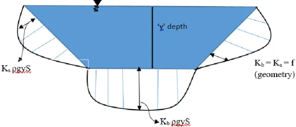
Figure 1 Shear stress distribution on the boundary of a trapezoidal channel

However, the variation of shear stress near wall and bottom is very different and thus may not be considered constant or equal to theoretical value. For example trapezoidal channel has shear stress distribution as shown in Fig. 1. The variation in the shear stress may vary with the bed width, side slope and even to the depth ratio. Similarly, the shear stress variation in the rectangular channel depends on the aspect ratio. Guo and Julien (2005) gave a graphical relation relating the average shear to ρgyS. Instead of using hydraulic radius flow depth is used since for wide channels, these would be almost identical.

Since we are generally concerned with the maximum shear stress at any point on bed or sides (e.g. to analyse the stability of a sediment particle), it is desirable to look at the maximum shear stress on the bed as well as sides (since the stability analyses for particles on sides and those on the channel are different). It is found that the maximum shear for the trapezoidal channel with side 2H:1V is around 75% of ρgyS on the sloping sides while it is almost ρgyS for the bed.

1.4 Stage discharge

The relationship within the water-surface stage (i.e. the water depth) and the coincident flow discharge in an open channel is known as stage-discharge relation or rating curve or just rating. This relationship is either empirical or theoretical which are can be used interchangeably since they are practically the same. The dependability on a rating curve as a tool is very high in surface hydrology since discharge data can be extrapolated from stage-discharge relationship at gauging station. However, the accuracy of this relationship is

(23)

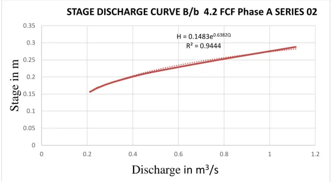
which necessitates an extensive theoretical background to establish a significantly accurate tool to compute discharge from measured flow depth. The wide applicability of the rating curve as a tool to estimate discharge in natural and/or artificial open channel and its extensive use in the field of hydrology makes it more demanding. Its application to the field of hydrology first came to knowledge in early XIX century where it was practiced to measure the discharge of a stream at suitable time using a current meter or other methods (Rantz 1982; ISO 1100-2, 1998). The corresponding stage is measured by regression or fitting the data set with power or exponential curve (see Fig. 2), a curve of the stage against discharge can then be useful to obtain the empirical equation depending upon the availability of data. One of the oldest methods of collecting current discharge data is to measure water level with gauges and then using the stage-discharge equation to estimate the flow discharge. The difficulty aroused during flood time is unrealistic for direct measurement of discharge in open channel in terms of risk of life, cost and time.

1.4.1 Hydraulics governing stage-discharge relationships

The stage-discharge relation in the open channel flow is dependent on the downstream condition from the gauge station. The channel conditions and characteristics understanding are very essential for the stage-discharge relationship and thus it is a very crucial component in developing rating curves. Three types of control are identified based on the channel and flow characteristics.

– A section control affects the low flow depths;

– A channel control affects the high flow depths;

– Both types of flow controls affect the intermediate flow depths.

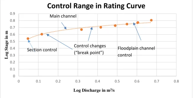
The sequence of section and channel control can occur at some stages. A section control is defined as the explicit cross-section of a channel, which is downstream from the gauge station having water level gauge regulating the relation between gauge height and discharge at the gauge. A section control such as rock ledge, a sand bar, a severe constriction in the channel, or an accumulation of debris can be identified as a natural feature section control. Similarly, a fabricated section control such as a small dam, a weir, a flume, or an overflow spillway is identified as the artificial section control. A pronounced drop of the water surface can be easily found in the field over section control, which signifies the meaning of control section itself, Fig. 3.

(24)

Figure 2 Stage Discharge Curve for B/b 4.2 Flood channel facility phase A series 02

Sometimes when the flow depth increase limitlessly these section controls get flooded and inundated in such a way that it no longer regulates the discharge in relation to the flow depth. At this particular instant, the drop is no longer visible, and flow either is controlled over another section control downstream or through the channel characteristics such as hydraulic geometry and the roughness of the channel downstream (i.e. channel control). A sequence of features throughout a reach downstream from a gauge is required in channel control. These features include channel size, shape, curvature, slope, and roughness. Dependency of the stage-discharge relation to the channel reach length can be extremely variable. A much longer reach is able to control the relation of the stage-discharge over the channel length of the flat or very milder channel, whereas very short channel reach may control the stage-discharge relation for the steeper channels. In addition, the magnitude of flow is also another parameter, which affects the length of channel control. The difficulty to define the length of a channel control reach is such a problem, which can be solved through numerical methods. As discussed above, the combination of the section and channel control are found in some of the specific stages, such as short range in stage between section-controlled and channel-controlled segments of the rating (Fig. 3). The development of stage-discharge curves where one control feature changes to another or combination of controls are possible or where number of measurement are handful, usually needs a wide understanding of the flow characteristics, in order to make a possible interpolation between measurements and extrapolation beyond respectively the lowest or highest measurements. This becomes

H = 0.1483e0.6382Q R² = 0.9444 0 0.05 0.1 0.15 0.2 0.25 0.3 0.35 0 0.2 0.4 0.6 0.8 1 1.2

Stag

e

in

m

STAGE DISCHARGE CURVE B/b 4.2 FCF Phase A SERIES 02

(25)

extremely reasonable where fluctuation of the controls is very high and have altered frequency time after time, resulting in a variation of the positioning of segments of the stage-discharge relation. The term transition zone is used where part of the resulting rating curve is regulated through both section and channel control. Both the controls acting simultaneously is usually a rare condition, though a combination control may be possible where each has a partial controlling effect. Plotting procedures are always used to identify the control and their behavior according to the stage-discharge relation. The characteristic of the transition zones, in particular, is distinguished through a change in slope or shape on the stage-discharge relation. The stage-discharge relationship for stable controls, such as fabricated structures are usually easy and have very less problem in terms of maintenance and calibration. For unstable controls problem arises in multiple when backwater occurs. In addition, segment of stage-discharge relation changes abruptly in unstable controls when severe flood or any other rare event occurs.

Figure 3 Schematic representation of controls range in rating curve

1.5 Flood hydrograph

The term hydrograph is a graphical representation of variation of discharge over a given period for a catchment area Fig. 4. It can also be stated as the response of a catchment area for a given input as rainfall intensity.

The total volume of water from a rainfall are not considered as a total input since the initial losses and the base flow (i.e. the flow through the ground water source) is excluded from

0 0.1 0.2 0.3 0.4 0.5 0.6 0.7 0.8 0.9 0 0.1 0.2 0.3 0.4 0.5 0.6 0.7 0.8 L o g Sta g e in m Log Discharge in m3_/s

Control Range in Rating Curve

Floodplain channel control

Section control Control changes (“break point”) Main channel

(26)

the volume and the remaining volume of water is denoted as the surface run-off or the quick response.

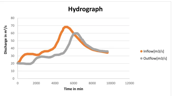
Figure 4 Hydrograph of inflow and outflow flood event 1994 River Brosna, Ireland

Iisrflow are also part of the quick response. As the name suggests the quick response are the volume of water that enters the stream immediately after the rainfall. As shown in the Fig. 5, a hydrograph has a rising limb, point of inflection, upper crest and then the recession limb. The characteristic of the curve shows the response of the catchment in a unique way where primarily during the rainfall the peak is built for over a period. The division of the

0 10 20 30 40 50 60 70 80 0 2000 4000 6000 8000 10000 12000 D isch ar ge in m 3/s Time in min

Hydrograph

Inflow[m3/s] Outflow[m3/s] 0 10 20 30 40 50 60 70 80 0 2000 4000 6000 8000 10000 12000 D isch ar ge in m 3/s Time in min

Hydrograph

Inflow[m3/s] Crest segment Rising Limb Dominated by direct run-off Recession Limb Point of inflection

(27)

base flow from the hydrograph is transitional and called as base flow separation, which have been proposed to distinguish surface run-off from the base flow.

1.5.1 Base flow separation

In many hydrographs analyses, a relationship between surface-flow hydrograph and the excess rainfall (i.e. rainfall minus losses) is sought to be established. The surface run-off hydrograph is obtained from the total run-off hydrograph through the technique called base flow separation. The graphical technique is established on locating the base flow recession points on the graph, which lies on the falling and the rising limb of the quick flow response. Another method called filtering techniques operate on the complete hydrograph data for obtaining the base flow hydrograph (Connected Water 2006).

1.5.2 Graphical separation method

Graphical techniques vary in complexity and they include:

 An empirical approach, which is based on the different parameters related to the characteristic of the catchment area Eq. 1.1. The basic idea behind this formulation is to find a point along the falling limb, which indicate the start of base flow recession on the curve.

D = 0.827 A0.2 (1.1)

Where, D is the number of days between the storm crest and the end of the quick response flow and A is the catchment are in square Kilometres.

 The constant discharge method assumes that a constant discharge of base flow occurs throughout the storm hydrograph.

 The constant slope method is established on the link between the start of the rising limb and the point of inflection on the falling limb. This method assumes the instant base flow response to the rainfall event, hence it is more suitable for the topography where base flow dominant.

 The concave method considers the initial recession in the base flow during the rising limb by projecting the decrease in the hydrograph trend prior to rainfall event to directly to the line joining the centre of the crest line perpendicular to horizontal axis. This projection is then connected to the point of inflection on the falling limb of a storm hydrograph.

(28)

Han (2010) suggested the constant discharge method and the constant slope method because of their simplicity and wide applicability.

1.5.3 Filtering separation methods

Another method, which is also used, for the base flow separation is the data processing or filtering procedures. This method uses the automation index of the base flow response of the catchment area. The ratio of base flow to the total flow calculated from the storm hydrograph smoothing and separation procedure using daily discharge are called as a base flow index (BFI) or reliability index (Tallaksen and van Lanen 2004).

1.6 Flood routing

A mathematical method to calculate variations in the magnitude and celerity of a flood wave when it proliferates down the river or across the reservoir is called flood routing. As the flood wave moves downstream its peak and the whole shape of the flood wave transforms throughout the movement (Tewolde 2005).

Considering the storage effect of the reservoir, the peak of the outflow hydrograph always have less attenuation in comparison to the inflow hydrograph. This relative decrement in the peak of the two consecutive hydrograph is attenuation Fig. 6. In addition, there is a translation, which indicates the delay in time of the peak discharge Fig. 6 while delay in travel time of the water mass moving downstream is called as lag time (Heatherman 2008).

Figure 6 Flood routing hydrograph for natural river Brosna, Offaly, Ireland Elbashir (2011) 0 10 20 30 40 50 60 70 80 0 2000 4000 6000 8000 10000 12000 D isch ar ge in m 3/s Time in min

Inflow-outflow Hydrograph

Inflow[m3/s] Outflow[m3/s] Lag time to peak Peak attenuation

(29)

The inflow hydrograph is considered as the flow of water at the upstream while the outflow hydrograph is the consequence of the inflow hydrograph at the downstream section. Flood hydrograph can be broadly classified as the reservoir routing and the channel routing (Subramanya 2009). However, the main difference explicitly depends on the outflow hydrograph for both the type i.e. when determined over the spillway is called reservoir routing and when estimated over the river reach is called channel routing (Chadwick and Morfett 1993).

1.6.1 Kinematic, dynamic wave speed and Froude number

In numerous past studies, researchers suggested that the travelling of flood wave is explained by the wave ‘celerity’ (Heatherman 2008). In an open channel flow, the dynamic celerity ‘cd’ is defined as the small disturbance or wave in the direction relative to the depth of the average velocity flow. To travel long enough wave must have low amplitude, long periods and negligible losses of energy.

cd = √𝑔𝑦 for wide rectangular channel (1.2)

cd = √𝑔𝐷𝑚 for channel in general (1.3)

Where, Dm = A/T i.e. ratio of Area of the channel to the top width of the channel called hydraulic depth.

From the equation above, cd is called as dynamic celerity and its unit is m/sec, g is the acceleration due to gravity m/sec2, y is the depth of the flow in m, A is the area of the channel in m2 and T is the top width of the channel in m.

The flow can be characterized by the dimensionless quantity called Froude number, which can be defined as the ratio of the average velocity ‘V’ of the flow to the dynamic celerity.

Fr =

𝑉

√𝑔𝑦 (1.4)

When the wave velocity surpasses the water velocity, the disturbance travel upstream and downstream, as well as the upstream depth of flow is affected by the downstream control. This case in particular is called as subcritical flow and the Froude number is less than one. In contrast to this when the flow velocity is more than the dynamic celerity than the supercritical flow is said to occur where Froude number is more than one and the disturbance now travel downstream only. The net possible case is when the velocity and dynamic

(30)

celerity is equal then the flow is called critical with Froude number equal to one (Chadwick and Morfett 1993).

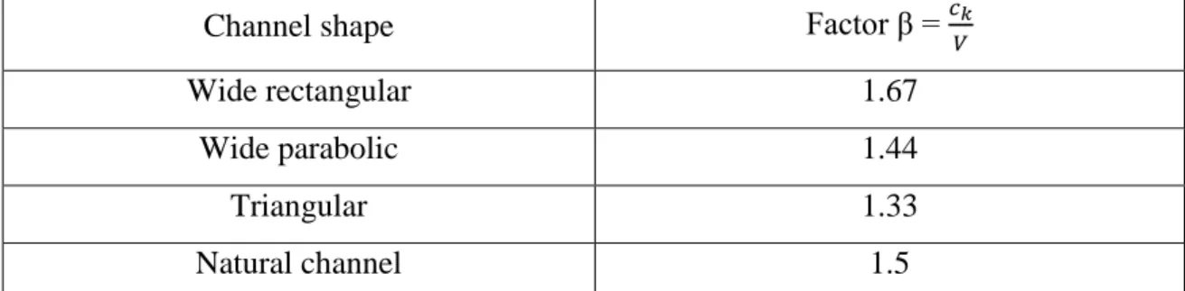
Kinematic waves ‘ck’ move with much lower velocities in contrast to the dynamic waves, which are characterized by quick attenuation, and higher velocities. Singh (1996) defined the Kinematic waves as the slope of the discharge-area rating curve. However, it can be estimated as the product of mean velocity and a factor called β. Table 1 shows the value for the factor β for various channel shapes.

Table 1 Factors for computing wave speed from average velocity (US Army Corps of Engineers, 2008

Channel shape Factor β = 𝑐_𝑉𝑘

Wide rectangular 1.67

Wide parabolic 1.44

Triangular 1.33

Natural channel 1.5

1.6.2 Distributed and lumped models

Commonly, the flood routing techniques are either lumped or distributed models. Lumped models consider complex parameters of flow behaviour between the upstream and downstream section of the channel. However, in the distributed models, more features of the flow behaviours are given at the points in between the reach located at the station from upstream to downstream section of the channel. Thus a model requiring lumped parameter are called hydrological routing, and flow routing through distributed parameter models is called hydraulic routing (Chin 2000).

1.6.2.1 Hydraulic method

When the flow computation is varied in both time and space (Mays and Tung 2002) then that type of flood routing technique is called hydraulic routing. Because of its computational ability over both space and time, this procedure is becoming popular for flood routing. Hydraulic routing is exercised through the continuity equation as well as the momentum equation of motion of unsteady flow (Subramanya 2009) Eq. 1.5 and 1.6.

(31)

Chapter 1 Introduction 𝜕𝐴 𝜕𝑡+ 𝜕𝑄 𝜕𝑥 = 0 (1.5) 𝑆_𝑓= 𝑆_𝑜− 𝜕𝑦 𝜕𝑥− 𝑣 𝑔 𝜕𝑣 𝜕𝑥− 1 𝑔 𝜕𝑣 𝜕𝑡 (1.6)

Where t is time, x is the distance down the channel, y is depth of flow, v is the mean cross sectional velocity, A is the area, Q is discharge, g is the acceleration due to gravity, 𝑆𝑓 is the

frictional slope, 𝑆_𝑜 is the bed slope, 𝜕𝑦

𝜕𝑥 is the longitudinal gradient of water profile, 𝑣 𝑔

𝜕𝑣 𝜕𝑥 is

the convective acceleration slope and 1

𝑔 𝜕𝑣

𝜕𝑡 is the local acceleration slope. The magnitude of

other terms are usually very less as compared to the bed slope 𝑆_𝑜.

This one dimensional continuity and momentum equation presented by the Barre de Saint-Venant (1871) are famously known as the St. Saint-Venant equations. Ignoring all other terms in the kinematic wave equation except pressure gradient term 𝜕𝑦

𝜕𝑥, the diffusive wave equation

becomes :

𝑆_𝑓= 𝑆_𝑜− 𝜕𝑦

𝜕𝑥 (1.7)

The pressure gradient term plays an important role in modelling the wave propagation and the storage effect within the channel for mild slope and steeply falling and rising hydrographs. Diffusive wave approximation equation simulates well, most of the flood wave travelling in the mild sloped river channels having some physical diffusion (Boroughs et al. 2002).

The full dynamic wave equation is those equations, which uses all the terms in the momentum equation. Its applicability is more often in the dam break analysis because it counters the backwater effects that other model neglect (Boroughs et al. 2002). The solution of such equations is more sophisticated, they use numerical modelling through high level computing techniques using implicit and explicit finite difference algorithm. Otherwise, it can be solved through the method of characteristics (Chin 2000). Other than this modelling techniques, one can also go for software packages which simulate momentum equation through different numerical schemes, commonly used are one dimensional HEC-RAS (Hydraulic Engineering Centre’s- River Analysis System) or MIKE 11 (DHI) to perform steady and unsteady flow river hydraulics calculations.

(32)

The demerits related to such model is the complexity of the model solution, problem of convergence and it often leads to the numerical unstable solution. Such model also requires costly computational resources and computation time. Other simplified methods were improved to assist the computation, generally hydrological method that is easy, requires low computational resources and less time consuming (Johnson 1999).

1.6.2.2 Hydrological methods

The basis of continuity equation i.e. the mass balance of inflow, outflow and the volume of storage remain conserved is used in hydrological methods for channel routing. This method of channel routing requires storage-stage-discharge behaviour to establish the outflow for each time step (Guo 2006). Hydrological method considers mathematical practices that initiate translation or attenuation to an inflow hydrograph (Heatherman 2008).

The equation presented below is continuity equation Eq. 1.8:

𝑑𝑆

𝑑𝑡= 𝐼(𝑡)− 𝑂(𝑡) (1.8)

where S is the storage between upstream and downstream in m3, t is the time in s and 𝐼_(𝑡)and

𝑂_(𝑡) are the inflow at upstream and outflow at downstream respectively in m3/s.

Over the finite interval of time between t and t+∆t Eq. (7) can be written in finite difference form as: 𝑆1−𝑆2 ∆𝑡 = 𝐼1+𝐼2 2 − 𝑂1+𝑂2 2 (1.9)

where subscripts 1 and 2 refers to two consecutive times t and t+∆t respectively (Chin 2000). A hydrological method, which initiates with continuity equation and comprises the dispersion form of the momentum equation, known as the MC (Johnson 1999) is used here for flood routing of Brosna River Offaly, Ireland (Elbashir 2011). The derivation and application of this method are discussed in further chapters.

(33)

1.6 Aim and Objectives

This research program has been pursued with the following principal aims:

- To study modelling techniques based on the Lateral discharge method using Reynolds Averaged Navier-Stokes Equation (RANSE) model for the computation of Stage discharge.

- To study the effects of secondary flow in compound channels through calibration coefficient Г and k which was given by Shiono and Knight (1991) and Ervine et al. (2000).

- To analyse the lateral variation of depth averaged velocity and boundary shear stress at different relative depths for compound channels.

- To substantiate the analytical solution results produced by four different methods with/without secondary flow term by means of a numerical method called K-ϵ (standard eddy viscosity model using ANSYS-Fluent).

- To study the application of hydrological flood routing technique using the constant variable MC method for a river Brosna Offaly.

- To examine the steady state and mass conservation condition of the constant parameter MC method using mass balance equation and storage equation based on prism and wedge storage principle.

Apart from the principal aims, following sub objectives can be enumerated as below:

- To analyze the depth averaged velocity distribution and the boundary shear stress distribution curves for non prismatic compound channels with a B/b ratio of 2.2 for three different relative depths as 0.100, 0.245 and 0.500.

- To analyze the depth averaged velocity distribution and the boundary shear stress distribution curves for non prismatic compound channels with a B/b ratio of 4.2 for three different relative depths as 0.111, 0.242 and 0.479.

- To validate the results for analytical and numerical solution using percentage error analysis for each relative depth.

- To validate the stage discharge curve using the data presented in the FCF phase A series 02 and 03 (www.flowdata.bham.ac.uk).

- To analyze the stage hydrograph plot for 8 Km reach of river Brosna Offaly taken from Elbashir (2011).

(34)

- To validate the results obtained from the constant parameter MC method with the two software packages, namely HEC-RAS (US Army Corps) and MIKE 11 (DHI).

1.7 ORGANISATION OF THE THESIS

This thesis has been organized into six chapters, including Introduction. Chapter 1 is the ‘INTRODUCTION’, which contributes a concise background of the rating curves, flood routing terminologies and aims & objectives of the present study undertaken.

Chapter 2 contains a brief appraisal of literature on compound river sections. All these subjects are considered in two different sections. The first section is about the different modelling techniques for depth-averaged velocity distribution, boundary shear stress distributions and stage discharge curve for compound channels. The second section is about different approaches of flood routing.

Chapter 3 describes the theoretical background of different modelling techniques and the important parameters related to them.

Chapter 4 deals with the results and discussions of the SKM with/without secondary flow term, K-method, extended SKM and K-ϵ model. It presents the results of depth averaged velocity distribution, boundary shear stress distribution and stage discharge curve for the two compound channel. In the next section, flood routing results are illustrated through the validation of the hydrologic routing technique (i.e. MC method) with the two software packages. Beside this water storage, analysis is done for the outflow hydrographs obtained.

Chapter 5 is error analysis, which compares the predicted depth averaged velocity with the measured depth-averaged velocity. Error analysis is also done to illustrate the contrast among all the contending models against extensive experimental datasets for ascertaining the efficiency of different models. The relative percentage error analysis is done in which the relative percentage error is plotted against the cross sectional lateral position. For outflow flood-hydrograph water conservation analysis is done and represented in the table.

In Chapter 6 some conclusions and scope for future work are drawn from the results obtained for the compound channels. The chapter also illustrates the scope of this study for the field engineers and for the future studies.

(35)

Chapter 2 Literature Review

Chapter 2

LITERATURE REVIEW

2.1 Stage Discharge, velocity distribution and boundary

shear stress

In the past several years, many attempts had been made in terms of mathematical modelling to predict the structure of turbulence in a compound channel incorporating the mass and momentum transfer over the interface region. A number of numerical models as that of Keller and Rodi (1988), Pasche et al. (1985), and the 3D algebraic stress model of Krishnappan and Lau (1986) has been undertaken along with many experimental work coming in between from Myers (1978) Rajaratnam and Ahmadi (1981), Knight and Demetriou (1983), Tominaga et al. (1989), Knight, and Abril (1996), and Knight (2006) in order to understand the structure of the flow. A number of empirical formulas are available in literature for the prediction of stage-discharge, velocity distribution and boundary shear stress but the dynamicity of such equation is very limited to very few channels or specific type of channel itself.

However, despite this progress an analytical solution for a compound channel, which will give depth-averaged velocity, boundary shear stress distribution in the transverse direction; together with the stage-discharge curve, has been given by different researchers such as Shiono and Knight (1988 and1991), Ervine et al (2000), Abril and Knight (2004), Omran (2008) Tang and Knight (2009) and Kordi et al. (2015).

Shiono and Knight (1988) gave an analytical solution based on the depth average eddy viscosity approach and momentum equation. The analytical solution is applied to steady and uniform flow in a compound channel and the results displayed confirms the capability of the model for the calculation of certain features of the flow sufficiently accurately for engineering design purposes.

Tominaga et al. (1989) shows that the secondary current produced and transformed due to anisotropy of turbulence, which results from the boundary conditions of the bed, the side wall and the free surfaces, as well as the aspect ratio of the channel and the channel

(36)

geometry. The three dimensional structure formed due to the coherent structures modifies the primary mean flow. The longitudinal vorticity equation explains and forms the basis of such a secondary current mechanism in closed and gravity flow. The measurement of coherent flow structure is necessary to understand 3D flow structure, but since the velocity of the secondary current is within a few percent of main channel flow it becomes difficult to measure them. The secondary current structure are very different in pressure and gravity flow. In an open channel flow free surface vortex and the bottom surface vortex are separated and forms the main reason in the dip of maximum velocity position and deceleration of mean velocity near surface. The secondary flow structure in rectangular channel are very much different from the secondary flow structure formed in trapezoidal channel.

Shiono and Knight (1991) again came up with the analytical solution but this time they have considered the secondary flow current denoted by Г. The calibration of coefficient of viscosity λ, friction factor f and secondary current Г has been done for the Flood Channel Facility FCF series 01-03 i.e. two stage trapezoidal channel. For the case of overbank flow, the experimental data from the FCF have provided comparable details for the 3D flow structures incorporated into the 2D analytical model through parametrization. The only realistic way of determining the depth-averaged secondary flow term has been shown through magnitude of boundary shear stresses and Reynolds stresses. The comparative intensity of secondary term and its impact on the lateral dissemination of the shear layer, have been shown to be unrelated of the relative depth, Dr (= (H-h)/H). In two-stage channels the point friction factors, f (=8τb/(ρUd2) are nearly uniform, but differ from main channel to floodplain due to varying depth. Dimensionless eddy-viscosity values λ, have been obtained through apparent shear stress, and depth averaged Reynolds stresses. Generally, coefficient of eddy-viscosity is taken as constant in overbank flow but in inbank flow consideration, it plays significant role.

Knight and Abril (1996) presented a philosophy for calibration of a river model through numerical simulation for overbank flow using three coefficients related to local friction factors, eddy viscosities and secondary flow. The numerical simulations of the lateral distributions of depth-mean velocity, boundary and Reynolds shear stresses give some useful insight into the calibration philosophy. The calibration philosophy of the model is found to be sensitive to friction factor f and secondary flow term Г values, particularly

(37)

insensitivity to dimensionless eddy viscosity λ ratios, wherein even constant values across the section may give satisfactory results.

Ervine et al. (2000) gave new model by rearranging the terms in lateral gradient of H(ρUV)d also called as secondary flow term. They also considered the effect of transverse velocity by considering the ratio of longitudinal and transverse velocity as a new constant k and replacing in the secondary flow term. This constraint k predominantly comprises the secondary cells and their intensity in the two-stage channel. They also showed that the value of k < 0.5% for straight compound channel flows and 2% k < 5% for meandering compound flows at least at the apex cross section. The model proposed has the plus point of being applicable to both straight and meandering two-stage channels by accepting an suitable value of k.

Abril and Knight (2004) gave a finite element model for depth-averaged turbulent flow using three hydraulic constraints governing local bed friction, lateral eddy viscosity and depth-averaged secondary flow for prediction of the rating curve relationship for inundating river. The subsequent lateral distribution of depth-averaged velocity are then integrated to give stage-discharge relationship. The comparison of the river flow model using finite element method with the coherence model of Ackers (1991 1992) in two study cases with homogeneous and heterogeneous roughness distribution helped to develop a calibration approach. It is also observed that from comparison of both models and experimental FCF data with homogeneous roughness, the coherence model yields inaccurate results in the prediction, which can be easily improved by using a higher value of the secondary flow term at low relative depths.

Knight et al. (2007) modelled depth-averaged velocity and boundary shear stress in trapezoidal channels with secondary flows incorporating some key 3D flow features into a lateral distribution model for streamwise motion. They suggested that the SKM is based on using a constant value of secondary flow term Г, commensurate with the lateral gradient of term H (ρUV) d and therefore each time sense of the secondary flow term Г changes, an additional panel is required. Therefore, separate four panels are essential for modelling secondary current flows in symmetric half of a simple trapezoidal channel. Aspect ratio b/H plays a significant role in determining the number of secondary flow cells. Although, accurate depth-averaged velocity distribution prediction, the corresponding boundary shear

(38)

stress does not always match the experimental data due to poor modelling of secondary current cells.

Omran (2008) justified that the SKM can account for 3D flow in simple and two-stage channels, is an easy method to program and can produce useful information required by river engineers, such as the stage-discharge relationship and lateral distribution of depth-averaged velocity and boundary shear stress. He also depicted that the accurate prediction of depth-averaged velocity not necessarily obtain the corresponding predicted boundary shear stress as precise as experimental data mainly due to poor modelling of the secondary current cells. The advantage such analytical model is that when no experimental data are available for the ungauged reach, the user can still model the reach through just allocating the roughness value because λ and Г are automatically determined across the channel via sense of semi-empirical equations.

Tang and Knight (2008) showed the application of the analytical solution to the depth-integrated Reynolds-averaged Navier-Stokes equation with an extra term encompassed to counter the effect of drag due to vegetation. An additional term drag force is used in the momentum equation to model the problem involving vegetation. The approach embraces the effects of bed friction, drag force, lateral turbulence and secondary flow via four coefficients f, CD, λ, Г respectively. The new analytical scheme applied to the lateral dissemination of streamwise depth-averaged velocity in a vegetated channel has been employed to symmetric two-stage channel with fractional roughness at the floodplain/ main channel edge, i.e. a single line of trees. It is illustrated in their work that the density of the vegetation affects the shear layer formation over the vegetated and non-vegetated region. In fact, a strong shear layer is generated over the rough surface and the transfer of momentum over interface enhances due to high density of vegetation.

Tang and Knight (2009) presented different analytical models of the depth-averaged Navier-Stokes equations applied to the gravity flow and validated those results with the experimental datasets. The models developed by Shiono and Knight (1988, 1991) are contrasted with those by Ervine et al. (2000) and Castanedo et al. (2005) by means of mathematical experiments on both simple and two-stage channels. All the three analytical solution are similar and approximately similar since they contain similar hydraulic constraints signifying boundary resistance via the bed friction factor f, lateral shear via dimensionless eddy viscosity λ, and the depth-averaged secondary flow via parameter Г or

(39)

K. They also demonstrated the significance of the secondary flow term by comparing results of those models where secondary flow term are not considered with the experimental data. The shortcomings with the assumptions of K model are also discussed. The coefficient K is arguably considered always positive even though the K-value can be either positive or negative, contingent on the rotation of secondary cell. The extended λ method with Г included, produced reasonably good results even though this model is found sensitive to λ-values.

Omran and Knight (2010) modelled the boundary shear stress distribution using depth-averaged Shiono Knight Method and shown that the poor modelling of secondary flow leads to the inaccurate results. To improve modelling by capturing the secondary current cell effects were analysed through the perturbation in experimental boundary shear stress dissemination. They indicated the poor modelling of the secondary flow term to be an important shortcoming in the prediction of boundary shear stress. The perturbation of the boundary shear stress distribution trend is visible in the aspect ratio larger than one, which in turn can be used as to decide the number, position and rotational direction of secondary current cells. They suggested that in rectangular channel, half the channel counted for modelling should be distributed into four panels to counter the effects of secondary current cells.

Azevedo et al. (2012) used the 2D Laser Doppler Velocimeter in an experimental compound channel to obtain the streamwise and vertical velocity component. They showed that the 3D behaviour of the flow is more noticeable. The results obtained are examined by comparing with the universal laws drawn for isotropic turbulent 2D fully developed open channel flow. They showed that the validity of the universal laws for 2D fully developed open channel flows in the upper interface and floodplain, although the coefficient has to be increased due to increase in turbulent intensity. The non-validity of the universal law in the lower interface or the main channel is mostly due to the strong secondary currents even if their coefficients are changed.

Al-Khatib et al. (2012) used the separate channel division methods in asymmetric two-stage channels with erratic floodplain widths and step heights. Three different interfaces, namely horizontal, vertical and diagonal is selected between the main channel and floodplain subsection. Then the discharge value in each subsection is evaluated in every interfaces together with the whole cross section. From the experimental results, it is observed remarked

(40)

that, none of the distinct channel approaches used assessed the calculated discharges correctly for the different ratio of depths in floodplain to main channel.

Zeng et al. (2012) presented different approaches to quantify the friction factor f and eddy viscosity coefficient λ for the application of the analytical solution and to improve the accuracy of the prediction of the lateral depth-averaged velocity in the trapezoidal compound channel flow. In their results, it is quite evident that the friction factor affects the accuracy of the solution. The coefficient of the eddy viscosity can be determined empirically since the precision of the solution has been less dependent on the effects of dimensionless eddy viscosity. Over the interface zone the difficulties to simulate the turbulent flow characteristics multiplies. The main cause of such challenging simulation is the discontinuity of the parameters especially in the interface zone and the channels is divided into different panels considering the cross section of the geometry rather than the internal structure of the turbulence.

Conway et al. (2012) offered a better technique for operating 3D computational fluid dynamics models to guesstimate the stage discharge and velocity distribution of straight open channel flow. In their approach, they used eddy viscosity k-ϵ turbulence closure model since in commonly used analytical solution model the coefficients are calculated through empiricism and vary with different flow conditions. The momentum transfer over the interface may or may not be taken into account, which potentially overestimate the conveyance capacity of the compound channels. The proposed approach is based on inputting (rather than calibrating) physically realistic resistance value and iteratively adjusting the downstream water depths until uniform flow conditions within a specified tolerance are established. They also suggested that the increase in relative depth of flow increases the momentum transfer due to difference in flow depth and velocity in the main channel and floodplain, which in turn over predict the flow ratio. Also, increasing depth increases the overestimation, which is more pronounced in roughened floodplain case.

Liu et al. (2013) presented an approach to model the depth-averaged velocity and boundary shear stress in a submerged and emerged both types of vegetation. In their study, they calibrated an extra coefficient to tackle the drag force due to the vegetation called coefficient of drag Cd. The analytical solution for the transverse variation of depth-averaged velocity is presented through the Shiono Knight Method (1991). Beside the calculation of an extra coefficient, secondary flow cells and eddy viscosity terms are also analysed and their effects

(41)

on the solution for the compound channel is presented. For dealing with the secondary flow term, the modified equation of Ervine et al. (2000) model is considered where coefficient K is taken into account. In their study, the most significant factor in the modelling approach is found to be secondary flow parameter K and also its sign, absolute value being determined by the rotational direction and the intensity of secondary flow cell plays an important role.

Jesson et al. (2013) examined a heterogeneous roughed bed in open channel flow through physical and numerical simulation. Depth-averaged velocity and boundary shear stress are experimentally calculated at four different cross sections by acoustic Doppler velocimeter and Preston tube technique respectively. The roughness aspects governs the behaviour of the flow and act as the source of vorticity, which is primarily established as local boundary shear stress and, in turn, affects imitates the momentum transfer and secondary flow in the channel. The flow field adjusts relatively quickly to the boundary roughness. The dissemination of vertical Reynolds stress is complicated and take longer to adjust over the change in boundary roughness unlike streamwise velocity component. Large fluctuation in the eddy viscosity model can be observed in the numerical simulation for the rough boundary conditions.

Yang et al. (2013) used the depth-averaged equation in a rectangular channel derived using the Newton’s second law established on an elemental water body. The analytical solution of the lateral variation of the depth-averaged equation is used which comprises the consequences of lateral momentum transfer and secondary flow in supplement to bed friction. The result shows the significance of the parameters used in the analytical solution and their influence together with boundary conditions used. The friction factor f in each subarea is estimated through the Colebrook-White equation and for a known geometry; secondary flow coefficient Г may be contemplated as uniform for various relative depths, but varies from the main channel and the floodplain respectively. The momentum transfer effects are prior and influencing in the shear layer region and may be practically overlooked outside the shear layer region.

Chao et al. (2013) conducted the experiments in the compound channel with vegetated floodplains for the investigation of the secondary flow characteristics. The variation in the vegetation in terms of size and shape changes the direction of rotation in the whole cross section. Meanwhile the intensities of the secondary flow current in the floodplain are stronger in comparison to the main channel when the flow depth is less. In the higher flow

A Study of Rating Curve and Flood Routing using Numerical Method

A STUDY OF RATING CURVE &

FLOOD ROUTING USING

NUMERICAL METHODS

Prateek Kumar Singh

Department of Civil Engineering

A STUDY OF RATING CURVE AND

FLOOD ROUTING USING

NUMERICAL METHOD

Master in Technology

Civil Engineering

Prateek Kumar Singh

215CE4286

June, 2017

Department of Civil Engineering

Department of Civil Engineering

National Institute of Technology, Rourkela

Certificate of Examination

(External Examiner)

Date:

Department of Civil Engineering

National Institute of Technology, Rourkela

Supervisor’s Certificate

DEDICATED TO

MY Nation

Declaration of Originality

Acknowledgment

Prateek Kumar Singh

Abstract

Contents

List of Figures

List of Tables

Nomenclature

Chapter 1

INTRODUCTION

1.1 General

1.2 Velocity distribution

1.3 Boundary shear stress

1.4 Stage discharge

1.4.1 Hydraulics governing stage-discharge relationships

Stag

e

in

m

STAGE DISCHARGE CURVE B/b 4.2 FCF Phase A SERIES 02

1.5 Flood hydrograph

Control Range in Rating Curve

Hydrograph

Hydrograph

1.5.1 Base flow separation

1.5.2 Graphical separation method

1.5.3 Filtering separation methods

1.6 Flood routing

Inflow-outflow Hydrograph

1.6.1 Kinematic, dynamic wave speed and Froude number

1.6.2 Distributed and lumped models

1.6 Aim and Objectives

1.7 ORGANISATION OF THE THESIS

Chapter 2

LITERATURE REVIEW

2.1 Stage Discharge, velocity distribution and boundary

shear stress