ATTRIBUTES
A Dissertation by
RASHEED ABDELKAREEM JARADAT
Submitted to the Office of Graduate Studies of Texas A&M University
in partial fulfillment of the requirements of the degree of
DOCTOR OF PHILOSOPHY
May 2004
ATTRIBUTES
A Dissertation by
RASHEED ABDELKAREEM JARADAT
Submitted to the Office of Graduate Studies of Texas A&M University
in partial fulfillment of the requirements of the degree of DOCTOR OF PHILOSOPHY
Approved as to style and content by:
Joel S. Watkins (Chair of Committee) Steven L. Dorobek (Member) John H. Spang (Member) Richard A. Startzman (Member) Mark E. Everett (Member) Richard L. Carlson (Head of Department) May 2004
ABSTRACT
Prediction of Reservoir Properties of the N-sand, Vermilion Block 50, Gulf of Mexico, from Multivariate Seismic Attributes. (May 2004)
Rasheed Abdelkareem Jaradat, B.Sc., Yarmouk University; M.Sc., Yarmouk University
Chair of Advisory Committee: Dr. Joel S. Watkins
The quantitative estimation of reservoir properties directly from seismic data is a major goal of reservoir characterization. Integrated reservoir characterization makes use of different varieties of well and seismic data to construct detailed spatial estimates of petrophysical and fluid reservoir properties. The advantage of data integration is the generation of consistent and accurate reservoir models that can be used for reservoir optimization, management and development. This is particularly valuable in mature field settings where hydrocarbons are known to exist but their exact location, pay, lateral variations and other properties are poorly defined.
Recent approaches of reservoir characterization make use of individual seismic attributes to estimate inter-well reservoir properties. However, these attributes share a considerable amount of information among them and can lead to spurious correlations. An alternative approach is to evaluate reservoir properties using multiple seismic attributes.
This study reports the results of an investigation of the use of multivariate seismic attributes to predict lateral reservoir properties of gross thickness, net thickness, gross effective porosity, net-to-gross ratio and net reservoir porosity thickness product. This approach uses principal component analysis and principal factor analysis to transform eighteen relatively correlated original seismic attributes into a set of mutually orthogonal or independent PC’s and PF’s which are designated as multivariate seismic attributes.
Data from the N-sand interval of Vermilion Block 50 field, Gulf of Mexico, was used in this study. Multivariate analyses produced eighteen PC’s and three PF’s grid maps. A collocated cokriging geostaistical technique was used to estimate the spatial distribution of reservoir properties of eighteen wells penetrating the N-sand interval.
Reservoir property maps generated by using multivariate seismic attributes yield highly accurate predictions of reservoir properties when compared to predictions produced with original individual seismic attributes. To the contrary of the original seismic attribute results, predicted reservoir properties of the multivariate seismic attributes honor the lateral geological heterogeneities imbedded within seismic data and strongly maintain the proposed geological model of the N-sand interval.
Results suggest that multivariate seismic attribute technique can be used to predict various reservoir properties and can be applied to a wide variety of geological and geophysical settings.
DEDICATION
This dissertation is dedicated to my beloved wife, Dr. Anne Gharaibeh, my sweet lovely angels, Rafeef and Abdelkareem, my parents, AbdelKareem Jaradat and Najwah Hijazi, and my parents in law, Dr. Ayesh Gharaibeh and Maha Gharaibeh.
ACKNOWLEDGMENTS
I wish to express my sincere gratitude to my advisor, Professor Joel S. Watkins, for his ample guidance, inspiration, friendship, and support throughout the course of this study. Special thanks also go to Professors Steven L. Dorobek, Mark E. Everett, John H. Spang and Richard A. Startzman for their cooperation, support and serving as committee members.
I would like to express my gratitude to Yarmouk University for their valuable sponsorship and providing the financial means to pursuing my degree. A word of thanks goes to the staff of the Department of Geology and Geophysics at Texas A&M University for their partial financial support and help to make this research project reach this final stage. Thanks are due to A2D Inc. for donating well log data. Their contribution represents an integral part to this study.
A similar vote of thanks and appreciation goes to all of my friends and colleagues for sharing tough and sweet moments at Texas A&M University. Special thanks, however, must be given to Dr. Ilyas Najmuddin, Dr. Eyad Masad, Mohammad Mohammad, Aslam Alomary and Mohammad Jaradat for their support and review of the manuscript.
I would like to express my sincere gratitude and thanks to my beloved wife, Dr. Anne Gharaibeh, for her endless support, patience and encouragement and for being a mother and a father to my kids during the past two years.
I would like to extend my thanks and admiration to my parents, my parents-in-law and my sisters for their invaluable support, corporation and sincere prayers. Finally, my sincere admiration goes to my beloved brother, Dr. Mohammad Jaradat, for his love, hospitality and encouragement. This dissertation would have been impossible without his assistance, care and love.
TABLE OF CONTENTS Page ABSTRACT ...iii DEDICATION ... v ACKNOWLEDGMENTS... vi LIST OF TABLES ... x LIST OF FIGURES... xi CHAPTER I INTRODUCTION... 1 1.1 Preface ... 1
1.2 Purpose of the study ... 3
1.3 Significance of the study ... 3
1.4 Objectives of the study ... 5
1.5 Location of the study area ... 6
1.6 Data base ... 6
II BACKGROUND... 9
2.1 Seismic attribute technology ... 9
2.1.1 Introduction ... 9
2.1.2 The use of seismic attributes to predict reservoir properties, a quantitative interpretation approach ... 11
2.1.3 Understanding seismic attributes ... 12
2.1.4 Potential challenges in reservoir characterization guided by seismic attributes ... 16
2.1.5 General review of seismic attributes applications... 20
2.2 General geology and stratigraphy of the study area ... 22
III METHODS OF INVESTIGATION... 32
3.1 Data loading and quality control ... 32
3.2 Post stack seismic processing... 32
3.2.1 Polarity definition... 32
CHAPTER Page
3.3 Tying well-to-seismic data (synthetic seismograms) ... 43
3.4 Edge enhancement attributes (variance cube and geoFeature mapping)... 47
3.4.1 Variance cube ... 47
3.4.2 GeoFeature mapping (MG) ... 49
3.5 Seismic attribute analyses ... 55
3.5.1 Seismic attribute extraction ... 55
3.5.2 Multivariate statistical analysis of seismic attributes ... 62
3.5.2.1 Data preparation ... 62
3.5.2.2 Principal component analysis (PCA) ... 65
3.5.2.3 Principal factor analysis (PFA) ... 68
3.6 Well log analyses ... 71
3.6.1 Multi-well normalization... 71
3.6.2 Petrophysical analysis ... 74
3.6.2.1 Shale volume (Vsh) estimation ... 74
3.6.2.2 Porosity estimation ... 76
3.6.2.3 Water saturation estimation (Sw) ... 78
3.6.3 Reservoir property summation ... 82
3.7 Geostatistical reservoir property estimation... 83
3.7.1 Background ... 83
3.7.2 Spatial analysis ... 85
3.7.3 Spatial anisotropy ... 87
3.7.4 Spatial mapping using kriging and cokriging methods ... 89
3.7.5 Spatial mapping workflow ... 93
3.8 Summary ... 94
IV RESULTS AND DISCUSSION ... 95
4.1 Structure and stratigraphy of the N-sand interval ... 95
4.1.1 Structural framework... 96
4.1.2 Stratigraphic framework... 96
4.1.3 Subconclusions... 112
4.2 Seismic attributes multivariate statistical analysis ... 115
4.2.1 Principal components analysis results... 115
4.2.2 Principal factor analysis results... 123
4.3 Well log analysis ... 131
4.4 Log-derived reservoir properties estimation using collocated cokriging... 134
4.4.1 Gross thickness mapping... 137
4.4.2 Net thickness mapping ... 152
4.4.3 Average gross effective porosity mapping... 168
CHAPTER Page 4.4.5 Net reservoir porosity thickness product mapping... 198 V CONCLUSIONS ... 214 REFERENCES CITED ... 216 APPENDIX ORIGINAL SEISMIC ATTRIBUTE MAPS OF THE N-SAND
INTERVAL... 225 VITA ... 235
LIST OF TABLES
Page Table 1. Paleobathymetric zones of indicator faunal assemblages of the
study area, showing a clear upward-shallowing trend within the
entire logged interval of middle and upper Miocene succession. ... 26
Table 2. GeoFeature Mapping allows different attributes to be computed within limits of a correlation interval. This table lists the different
attributes and their description. ... 51
Table 3. A summary table listing the 18 different extracted seismic
attributes and their definitions and common applications. ... 60
Table 4. The different reservoir properties estimated over the N-sand
interval and their descriptions. ... 82
Table 5. Results of the eigenvalues and the proportion of variance
explained by each principal component. ... 117
Table 6. Principal components loadings for 18 extracted seismic attributes
representing the N-sand interval. ... 120
Table 7. Principal component factor analysis of the correlation matrix. The upper table shows the unrotated factor loadings and
communalities. The lower table represents the final results of PFA loadings after Varimax rotation and sorting. Loadings less than 0.3 were considered not important. The communality of each attribute is the portion of the total variance shared with the
remaining attributes (Dunteman, 1989). ... 124
Table 8. Summary of N-sand interval well log properties of Vermilion 50
LIST OF FIGURES
Page Figure 1. Distribution of reserves and production data by geologic age of
central GOM region. ... 4
Figure 2. Location of the study area. The seafloor is less than 20 ft deep and is just a few miles south of the coasts of Louisiana. Area shaded in red denotes the portion of the seismic data used in this study (after Zeng
et al., 2001)... 7
Figure 3. Seismic basemap, limits of the area of interest (shown in blue border line), lease blocks and wells of Vermilion 50 (left) and Tiger Shoal
fields (right)... 8
Figure 4. The various types of post-stack seismic attributes derived from the basic seismic information of time, amplitude, frequency, and attenuation. The window can be a constant time interval, a constant interval hung from one horizon, or the interval between two horizons
or depth (after Brown 2001)... 10
Figure 5. Schematic representation showing the complex relationships
between the different physical factors affecting seismic properties... 14
Figure 6. Schematic wavelet of typical wavelength for a) laboratory measurement, b) sonic logging tool, and c) seismic data (after Yang
and Stewart, 1997)... 18
Figure 7. Map showing the regional distribution of major Tertiary depocenters in the northern Gulf of Mexico. Study area location is
outlined on the map rectangle. (after Martin, 1978). ... 25
Figure 8. Dip oriented seismic section of the total Miocene succession penetrated by the wells of Vermilion 50, showing a clear transition from deep slope deposits into proximal shelf depositional settings. Color scale indicates the following upward-shallowing trend; Slope,
Page near shelf edge, distal shelf, middle shelf and proximal shelf. N-sand
interval is highlighted by the red arrow at the upper/middle Miocene
boundary. Black indicates positive seismic polarity ... 28
Figure 9. Dip oriented seismic section of the proximal shelf of the upper Miocene, showing various patterns of channeling and incision within a marginal marine setting. Horizontal scale = 20 trace/inch and vertical scale = 7.5 inches/second. Time slice horizontal scale = 100
trace/inch. ... 31
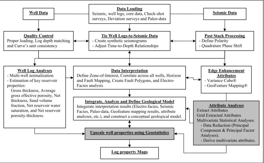
Figure 10. A schematic workflow outlining the main procedures involved in this study. Shaded procedures have their detailed workflows, illustrated in Figures 11 and 12. The double-headed arrows indicate a
two-way feedback process. ... 33
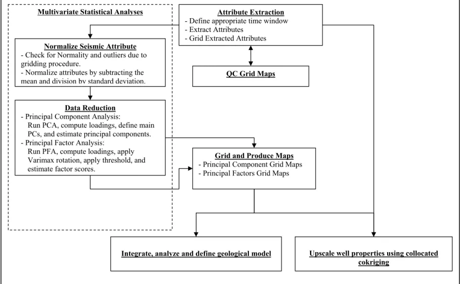
Figure 11. A schematic workflow outlining the main steps of the attribute analysis procedure. The double-headed arrows indicate a two-way
feedback process. ... 34
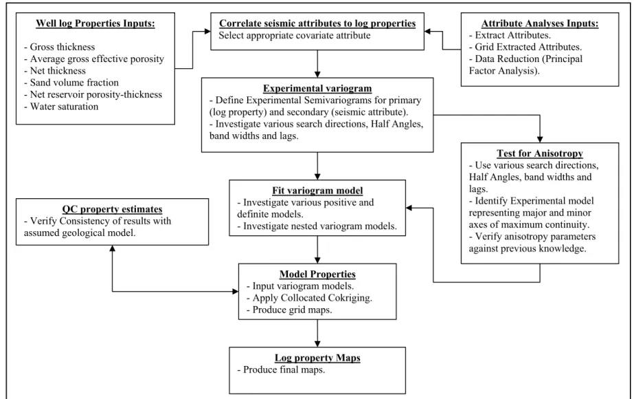
Figure 12. A schematic workflow outlining the main steps of the upscaling procedure by using collocated cokriging method. The double-headed
arrows indicate a two-way feedback process. ... 35
Figure 13. The conventional detention of seismic polarity adopted by the
Society of Exploration Geophysics (SEG)... 36
Figure 14. A deterministic wavelet extracted in the region of well 31_6 with a dominate frequency of 17Hz, suggesting a reverse polarity definition
and that the data is processed to an almost zero-phase state. ... 37
Figure 15. Synthetic 2D-forward modeling of a seismic response of N-sand reservoir produced by a reversed polarity Ricker wavelet and a dominate frequency of 20MHz. Notice the good match between the N-sand reservoir and the trough of the seismic signal. a) The geological model used as an input (blue curve represents a Gamma-ray, and red curve represents delta-time log), and b) represents the
Page results of the GMAplus 2D seismic modeling. ... 38
Figure 16. A time domain representation of the extracted wavelet of the original data set. The best-fit location (where the correlation reaches a maximum is marked by the blue crosshair), is located around the trace 356 and optimal lag of 48.0ms. This defines the location of best match between the seismic and the reflection coefficient series from
the borehole. ... 41
Figure 17. A time domain representation of the extracted wavelet of the -90q phase shifted data set. The best-fit location (where the correlation reaches a maximum is marked by the blue crosshair), is located around the trace 124 and optimal lag of 8.0ms. Compared to the Figure 5, it is clear that a quadrature phase shifting will enhance the
process of interpretation and tie between wells and seismic data. ... 42
Figure 18. The original check-shot survey data, 10 wells, representing the whole area of seismic coverage. Surveys from adjacent blocks (236, 241, and 242) showing the same trend as well, indicating a very smooth velocity model. Well names are shown on the legend.
221_99 is an average survey model supplied by TEXACO... 45
Figure 19. A typical synthetic seismogram of well 31-6. N-Sand is highlighted
by cyan color. ... 46
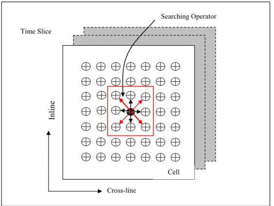
Figure 20. A schematic presentation of the different components used in variance cube computation. Each cell is composed of 3, 5, or 7 traces or a combination of them. The searching operator shows the possible
spatial options to compute the variance values. ... 48
Figure 21. A 4 layout comparison between the original (a&b) and variance cube (c&d) data. The posted inline is inline number 1351, and depth the time slices is 2012ms. Variance cube data improves the accuracy of structural interpretation. Variance cube time slices (d) have the superiority in illuminating discontinuities more sharply when
Page Figure 22. A schematic diagram showing the 2 different options of datum
selection available in GeoFeature mapping tool. 1) the
Depth-to-Depth and 2) the Horizon-to-Depth-to-Depth options... 52
Figure 23. The different spatial search directions available in GeoFeature Mapping tool. These different searching patterns allow illuminating obscured features oblique to the normal inline and cross-line seismic
lines. ... 52
Figure 24. A quality factor attribute map created using a window offset of 100ms above the N-sand interval, showing the progress of valley incision and channeling patterns (yellow color) across an ancient marine shelf substrate (red color). Each map represents a window
step 5ms... 54
Figure 25. Vertical seismic section showing the two phantom horizons, in red color, centered on an interpreted blue event of the N-Sand. These two phantoms are used to define the upper and the lower boundaries
for attributes extraction. (Troughs appear in hot color shades)... 55
Figure 26. A map representation showing the origin of interpretation. Interpretation shown in red represents the manually picked seismic traces. Densely picked areas represent the regions of weak signal-to-noise ratio, low lateral continuities, due to attenuation or fault
distortion... 57
Figure 27. A map representation showing of the quality of the autopicking process. It is a measure correlation between autopicked interpretations and adjacent manually picked traces. The quality of the autopicking is highly correlated to its seedpicks (generally
>90%). ... 58
Figure 28. A map presentation of the Arc length seismic attributes, extracted within an interval of 5ms above and below of the two phantom horizons. Anomalies characterized by higher arc length values
Page Figure 29. Normal density distribution plots showing (a) Bandwidth rating
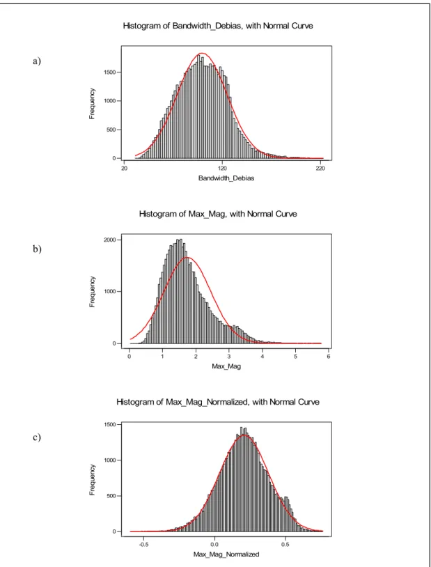
(debias) attribute; (b) Maximum magnitude attribute; and (c) Maximum magnitude after natural log transformation. Bandwidth debias attribute shows a clear normal distribution pattern, meanwhile maximum magnitude is positively skewed distribution, which is
transformed into normality by using a natural log transformation... 64
Figure 30. Correlation matrix for the 18 extracted attributes. The degree of correlation between some attributes indicates that applying principal component analysis would be beneficial to reduce the dimensionality
of the data base. ... 67
Figure 31. Neutron porosity log histogram. The standard histogram is correlated well log data. Key data represent data of the following wells: 30_1, 30_4, 210_93 and 31_4. The target data is from well 31_12. Notice that no normalization is needed in such case.
Frequency is plotted on the vertical axis. ... 72
Figure 32. Neutron porosity log data of well 31_5 before normalization (A),
and after normalization (B). ... 73
Figure 33. Density porosity-neutron porosity crossplot of well 30_4. Gas effect tends to shift the sample points up the 45º line, thus lowering the neutron porosity values. Shale free and water-filled samples fall on the 45ºline. The effect of shaliness tends to displace the sample points below the line, depending on the type of clay present, thus increasing the neutron porosity values. Highlighted points are those shown in the adjacent strip log presentation. (Overlay is modified
after Hunt and Pursell, 1997). ... 75
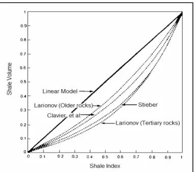
Figure 34. Nonlinear shale volume chart (after Alberty, 1992). ... 76
Figure 35. Strip log presentation of wells 30_2 and 30_4 indicating a good correlation is taking place between core porosity and density
Page Figure 36. Core-to-log scatter plot illustrating the correlation between core
porosity of wells 30_2 and 30_4 and density porosity logs. The highlighted points represent shale-free samples within the N-sand interval. Fitting is produced by reduced major axis regression
technique. ... 77
Figure 37. A multi-well pickett plots comparison between a clean sand model with Vsh < 5% (A), and shaly-sand model with Vsh=15-20% (B). In
the clean sand case Rw=0.01 ohm-m, while in the shaly-sand model
Rwe=0.018 ohm-m. Accordingly, the dual water motor is the right
model to calculate water saturation (Hunt, 1997). ... 80
Figure 38. Strip log final presentation of well log analyses results of well
30_4. ... 81
Figure 39. A typical plot of an experimental variogram and the fitted variogram model. Range (R), the nugget (C0) or the nugget effect
and the sill (C) are known as variogram attributes... 86
Figure 40. An example of ellipse fitting case of 12 different directional variograms. A major axis represents the direction of maximum continuity. The minor axis represents the trend of minimum
continuity... 88
Figure 41. Structure map of the top of N-sand interval. Major growth faults are highlighted by black arrows. Time-to-depth conversion was achieved by using collocated cokriging approach. Wells shown in
red were used in the time-to-depth conversion. ... 97
Figure 42. Dip-oriented seismic section across fault A illustrating a gentle rollover structure of the of Vermilion 50 field. The distance between
the posted wells equals to 1.96 miles. Troughs appear as hot colors. ... 98
Figure 43. Dip-oriented cross section illustrating the forth medial third-order sequence composed of lowstand, transgressive and highstand system tracts. The N-sand interval represents the uppermost lowstand
Page system tract incised valley unit. (after Hentz and Zeng, 2003)... 99
Figure 44. Quality factor map of the N-sand interval showing the general depositional setting of the interval. Vermilion 50 field is associated with a major incised valley system developed in the western side of the study area. The boundaries of the incised valley are shown with dashed red line segments. The eastern side of the valley defines a main channel system developed into a lowstand deltaic system. The area delimited by dashed circle identifies a second-order fluvial channel system feeding the major trunk of the valley. The Tiger Shoal field is slightly affected by incision, but reflects a general
sediment bypass activity... 102
Figure 45.Seismic amplitude map on the right corner shows clear anomalies of higher negative amplitude. These anomalies are associated with regions of maximum offset across the growth fault suggesting sediment focused accumulations and subsidence activity. The effect of subsidence is manifested in higher zones above the N-sand Interval. A and B illustrates the spatial (time-slice 2353ms) and lateral distribution of the major trunk region of the incised valley, respectively. The orientation of the seismic section is shown with
yellow trace across the seismic amplitude map. ... 104
Figure 46. Quality factor map draped over 3D time surface structure of the N-sand interval. Postulated sediment dispersal pathways across the western and the eastern regions are shown with white colored traces. Distribution patterns indicate a general sediment bypass behavior across syndepositional fault systems, which is a typical pattern of lowstand systems tracts. The western region was able to attain more sediment compared to the eastern region. The major domal structure associated with the Tiger Shoal field prevented the far-east footwall blocks (highlighted by dashed black arrows) from receiving sediments representing remnant marine shale flood plains. Fault traces are high lighted in dashed red color. Sediments pathways are
highlighted with white color. ... 105
Figure 47. A structural cross-section across fault (B) indicated a pronounced localized growth stratigraphy of N-sand interval in relation to
Page Figure 48. Seismic arc length attribute map showing exposed remnant marine
flood plains. A major interfluve plain located in the center of the study area suggests that the western major incised valley and the eastern region were fed by separate distributaries. Black arrows represent probable trend of the distributary systems feeding the western and eastern incised valleys. The orientation of the axis of distributary feeders was concluded based on subsidence signatures across seismic section parallel to the main growth fault. Unfortunately, the lack of seismic coverage from the eastern side
imposes limitation on this interpretation. ... 107
Figure 49. Comparison between the mean values of the different well log-derived reservoir properties of Vermilion 50 (n=19) and Tiger Shoal (n=19) fields, indicates that the western and the eastern regions of
the study area have different depositional properties... 108
Figure 50. Passive margin incised valley systems of the Cenozoic of the GOM, can be classified into 4 major end-members, based on the interaction between the amplitude of sea level fluctuations relative to the elevation of the shelf/slope break and rate of sediment supply.
(after Bowen, et al., 1993)... 108
Figure 51. A set of quality factor seismic attribute maps generated relative to the lower boundary of the N-sand interval using a 5ms sample interval. These maps represent the history of progressive incision and deposition taking place across an exposed shelf during a major lowstand conditions. The oldest phase is presented in map (A) and the final phase is presented in map (j) which culminates the lowstand period by a wide marine transgression episode defining the middle section of the 4th medial third order sequence (Hentz and
Zeng, 2003), shown in Figure 44. ... 110
Figure 52. Acoustic amplitude map of the N-sand interval overlain by time structure contour map. Note that the boundaries of the incised valley
confirm to the time structure contour line. ... 114
Figure 53. Correlation matrix plot illustrating the degree of correlation between extracted seismic attributes. Correlated attributes share
Page information between them which can mask the level of correlation
between them and well log reservoir properties. Red color denotes
clean sand deposits and green color represent shaly deposits. ... 116
Figure 54. Scree plot presentation of the results of the first 10 PC’s. The first 3 PC’s represent 0.89 of the total variance in the original 18 seismic attributes. Values posted above bars represent the cumulative variance value (Table 5). Seismic attribute grid map contains 56715 samples and 2505 missing values. Correlation matrix was used in the
analysis. ... 117
Figure 55. Principal components loading plot illustrating the main seismic attributes imposing significant load on each transformed PC. Note that the first three represent 0.89 of the total variance. The full
loading values are listed in Table 6. ... 118
Figure 56. Comparison between the PC-1 (a) and the mean trough amplitude attribute (b). Note that PC-1 was able to reduce noise and to highlight a set of anomalies which are related to changes in lithology
or hydrocarbon bearing deposits. ... 121
Figure 57. Principal components two (a) and three (b). Compared to PC-1 which is more sensitive to hydrocarbon accumulation and related lithology changes, PC-2 and PC-3 more sensitive to internal
heterogeneities and cyclicity within the time window. ... 122
Figure 58. PFA loadings matrix comparison between unrotated loading (a) rotated loadings using Varimax (b) and rotated and sorted loading with a cutoff value of (0.3). Plot (c) is much easier to interpret and
indicates that the results of PFA were comparable to the PCA. ... 125
Figure 59. PF-RT-1 is the first rotated principal factor after Varimax rotation. The upper channel region of the incised valley shows a possible lateral migration of the axis of distributary channels. The upper section of the of well 30-1 and 30-6, not shown in section, received marginal sand deposits compared to adjacent wells located with
Page Figure 60. PF-2 (A) and PF-3 (B) map presentation with Varimax rotation
applied. These PF’s reflect possible heterogeneities similar to PC-2
and PC-3, but they show fewer variations due to tighter scale. ... 128
Figure 61. LFSC-1 is the linear factor score combinations of the main loaders of PF-1 (upper) and LFSC-2 is the linear factor score combinations
of the main loaders of PF-2 (lower). ... 129
Figure 62. Normal density plots of the multivariate seismic attributes. PC’s
tend to have wider ranges compared to PF’s... 130
Figure 63. Collocated cokriging variance as a function of the coefficient of correlation, assuming normalized primary and secondary variable inputs. An increase in correlation coefficient between primary and secondary data will minimize the amount of variance associated with collocated cokriging. Note that collocated cokriging will fall to a simple kriging case, when the correlation coefficient equals to 0.0. Hence, secondary data contribution is ignored. (after Doyen et al.,
1996).V2SK is simple kriging estimation variance. ... 135
Figure 64. Dip- oriented seismic section across Tiger Shoal field. N-sand interval shows a sagging effect due to overlaying stacked gas saturated sediments. Additionally, the proximity of the wells to the fault plain produces low correlative relationship with reservoir log
properties. SP logs are posted in red. ... 136
Figure 65. Seismic amplitude map of the western region of the study area. In general, wells located up dip of the incised valley have higher gross sand thicknesses. The postulated boundaries of the main incised channel are shown with dashed orange line. A subsidiary distributary system is shown to the west of the major trunk of the incised valley. Well 210-95 is located off the incised valley and was discarded from spatial analysis studies. The lower map shows the whole western region which is defined by the dashed yellow border. Black arrows indicate possible incised valley boundaries due to successive
Page Figure 66. Crossplot between the gross thickness (ft) and TWT Time (s).
Updip wells, highlighted by the dashed ellipse, are characterized by higher gross thickness measures while down dip wells show a
general decrease in gross thickness. ... 139
Figure 67. Spatial analysis parameters of gross thickness property of Vermilion 50 wells. The direction of maximum continuity is parallel to the regional strike of the region which is correlated to the local
depositional strike orientation. ... 140
Figure 68. Correlation coefficient plot of the absolute value of the correlation coefficient (r) between gross thicknesses inferred from wells and seismic attributes. Gross thickness property showed good correlations with instantaneous phase (r=0.65) and PC-17 (r=0.73). Note that original seismic attributes were standardized by subtracting the mean and division by the standard deviation value. LFSC-1 is a
linear factor score combination of PF-RT-1. ... 141
Figure 69. Instantaneous phase in Vermilion 50 area of the study area (a) showed good correlation with well-log derived gross thickness (b).
The correlation coefficient value seen in the plot is -0.65. ... 142
Figure 70. The multivariate seismic attribute PC-17 of the western region of the study area (a) correlate better with gross thickness well-log derived gross thickness (b). Compared to the cross-pot shown in Figure 69, Figure 70 showed less spread for the down dip wells
where there is more well control. ... 144
Figure 71. Bar chart illustrating relative contributions (loading) of seismic attributes in PC-17. PC-17 is mainly a weighted linear combination of mean magnitude, minimum amplitude and RMS amplitude. Note that the relative contribution for instantaneous phase to PC-17 is
negligible. ... 145
Figure 72. Comparison between gross thickness estimates produced by using instantaneous phase attribute (a) and gross thickness estimates produced by using PC-17 (b). Blow-ups of these maps are shown in
Page Figures 73 and 74, respectively. Note that gross thickness estimates
at footwall region showed higher values in (a) than that of (b). ... 146
Figure 73. Gross thickness estimate of the N-sand interval from instantaneous phase attribute. Areas highlighted by dashed circles showed high estimates for gross thickness compared to PC-17 estimate of gross
thickness (Figure 72). ... 147
Figure 74.Gross thickness estimate of the N-sand interval from PC-17 showing south-trending linear channel belts of maximum gross thickness which are separated by interchannel areas. These linear trends are strongly correlated with the distribution of historic drilling activates within the area. Figure 75 shows an enlarged version of the central delta deposits. Wells highlighted with yellow triangles represent historic drilling activity within the study area (www.A2D.com, 2003). Wells shown in red stars are these available
to this study. ... 148
Figure 75. An enlarged plot of the central area of Figure 74. It is possible to distinguish linear trends of high gross thickness values (Figure 74). These trends are interpreted as distributary channels of lowstand deltaic deposits of the valley fill which are strongly correlated with
the aerial distribution of historic drilling activates within the area... 150
Figure 76. Correlation between measured values of gross thickness and collocated cokriging estimates of gross thickness produced by instantaneous phase attribute (a) and PC-17 (b). Although the same spatial model is used estimates produced by PC-17 showed less spread and a slightly higher correlation coefficient value (r=0.98 vs.
0.96) compared to the original seismic attribute. ... 151
Figure 77. Seismic amplitude map of the western region of the study area overlain by a bubble layout presenting the spatial distribution of well-log derived of net thickness values of N-sand interval. The up dip and western side wells of the incised valley have higher net thicknesses. Postulated boundaries of the incised channel to delta are
Page Figure 78. Spatial analysis parameters of net thickness property of Vermilion
50 wells. ... 154
Figure 79. Correlation coefficient plot of the absolute value of the correlation coefficient (r) between net thickness and the various seismic attributes for the wells located within the incised valley (n=18). Net thickness property showed a good correlation with the sum of magnitude (r=0.50) and the PC-14 (r=-0.67). Note that the original seismic attributes are normalized by subtracting the mean and
division by the standard deviation value. ... 155
Figure 80. Standardized sum of magnitude seismic attribute of the western area of the study area (a) showed the best correlation with net thickness well-log derived gross thickness (b). The correlation coefficient value seen in the scatterplot is the absolute value of
r=0.50. ... 157
Figure 81. Multivariate seismic attribute PC-14 of the western region of the study area (a) shows better correlation with net thickness (b). Compared to the scatterplot shown in Figure 79, Figure 80 showed less variability around the regression line. Note that well 210-95 is located out side the incised valley system. The wells 12 and 31-21 were turned off because they are highly deviated from the general
trend shown by the rest wells. ... 158
Figure 82. Bar chart illustrating the relative contribution of each seismic attributes in PC-14. Largely, PC-14 is a weighted linear combination of average trough amplitude and sum of magnitude. The higher relative contribution of the average trough amplitude compared to the sum of magnitude attribute suggests that this multivariate attribute is trying to enforce the amount of the seismic information coming mainly from the trough region of the seismic signal. Synthetic seismogram modeling indicated that N-sand interval is
associated with seismic trough portion. ... 159
Figure 83. PC-14 and PC-17 have similar response within sharp boundary clean sand deposits. The inverse relationship shown between PC-14 and net thickness ensures that PC-14 will correct for possible errors
Page encountered during attribute extraction in poor boundary deposits
due to sampling events from the upper peak. Thus, PC-14 will respond to the net thickness rather than the gross thickness which is fully accounted for by PC-17 and partially by the sum of magnitude attribute. Note the separation seen between PC-14 and PC-17 in poor upper boundary in the center of the upper scale bar, and minimal separation at sharp boundary regions. Well logs are SP log and the
right boundary does not reflect the shale baseline. ... 160
Figure 84. Comparison between net thickness estimates produced by sum of magnitude (a) and net thickness estimates produced by using PC-14 (b). Figures 84 and 85 shows enlarged versions of map (A) and map (B), respectively. Note that net thickness estimates showed smoother
behavior in (a) than that of (b). ... 162
Figure 85. Net thickness estimate of the N-sand interval produced by sum of magnitude attribute as a secondary data. The highlighted area by the dashed-line circle shows high estimates for net thickness compared
Figure 84. ... 163
Figure 86. Net thickness estimate of the N-sand interval produced by using PC-14. Net thickness of PC-14 maintains the anticipated roughness associated with the lithology and depositional systems existing within the incised valley and correlates will with historic drilling activities of the study area. The black dashed line highlights a possible boundary defining the edge of delta front deposits of the incised valley fill. Note that the anomalous region shown by the net thickness estimates of the sum of magnitude is not evident in the
results of PC-14, shown in red dashed circle. ... 164
Figure 87. Arbitrary dip-oriented seismic section (a) and the net thickness map produced by sum of magnitudes (b). The highlighted anomalies existing within the southern part of the incised valley are mainly related to possible hydrocarbon saturated sediments. The marked bright spot signature on the vertical seismic section supports this conclusion. The correlated behavior between PC-17 and PC-14 over this region, note scale bar in (a), indicates that estimates of gross and net thicknesses produced by using PC-17 and PC-14 should be equal.
Page Figure 88. Correlation between measured values of net thickness and
collocated cokriging estimates of net thickness produced by sum of magnitude attribute (a) and PC-14 (b). Note that both approaches gave similar results for the wells located within the incised valley. As for the region located out side the valley, the sum of magnitude approach highly overestimated net thickness at well 210-95. Note also that both approaches gave accurate estimates for net thicknesses
at the wells 31-12 and 31-21 which were turned off (b in Figure 80)... 167
Figure 89. Scatterplot between effective maximum porosity as a function of depth and the well-log derived estimate of effective porosity before (a) and after (b) correction for the outliers: 50-D-2(7), 218-10 and 218-14. B). Note the goodness of fit in (B) equals to 0.75. This scatterplot indicates that the well log estimates of effective porosity
are acceptable and considered representative of the N-sand interval... 169
Figure 90. Average amplitude map of Vermilion 50 field overlain by a bubble plot showing the distribution of well-log derived effective porosity estimates of the N-sand interval. The spatial variation between the estimated effective porosity values is minimal but the up dip and western side wells of the major channel within the incised valley have higher Ieff. The postulated boundaries of the incised valley are shown with dashed orange line. The shaded area represents a trend
of high Ieff sediments of high energy depositional conditions. ... 171
Figure 91. Spatial analysis parameters of gross Ieff of Vermilion 50 wells. ... 172
Figure 92. Correlation coefficient plot of the absolute value of correlation coefficients |r| between Ieff and the various seismic attributes for the wells located within the incised valley (n=18). In general, all amplitude-based attributes show good correlation with average porosity. Accordingly, PC-1, PF-UR-1 and PF-RT-1 will show high correlations since amplitude-based attributes are the main loaders for these multivariate attributes. The best correlation is shown by the PF-RT-1 (r=-0.72). and the sum of magnitude (r=0.59) original
Page Figure 93. Standardized average amplitude seismic attribute map (a) showed
the best correlation with gross effective porosity (b). ... 175
Figure 94. Multivariate seismic attribute PF-RT-1 (a). The correlation coefficient estimate and regression pattern shown in (b) is comparable to that shown by the average amplitude (Figure 92). Compared to spatial map distribution shown in Figure 93, PF-RT-1 enhances the level of contrast between incised valley sediments and
adjacent marine shelf sediments and across the footwall region. ... 176
Figure 95. Bar chart illustrating the relative contribution of each seismic attributes in the principal factor PF-RT-1. Amplitude-based seismic attributes represent the highest loaders to PF-RT-1. Minor contributions are offered from seismic arc length, the number of zero crossing and the ratio of positive to negative seismic attributes. These minor attributes are sensitive to internal stacking heterogeneity within an interval (Table 3) suggesting that this factor is trying to screen those regions characterized by higher gross
effective porosity and higher internal heterogeneity... 178
Figure 96. Comparison between gross thickness estimates produced by using instantaneous phase attribute (a) and gross thickness estimates produced by using PC-17 (b). An enlargement of these presentations
is shown in Figures 70 and 71, respectively... 179
Figure 97. Gross effective porosity estimate of the N-sand interval produced by average amplitude seismic attribute as a secondary data. The elevated estimates of gross effective porosity within Area 1 and 2 are mainly attributed to saturation effect. The Figures 86 and 87 show seismic cross-sections across area 1 and area 2 respectively. It is evident that both areas are defining positive topographic relief that results in closures capable of trapping hydrocarbons. Note the
topographic relief and amplitude signature across the both areas... 180
Figure 98. Gross effective porosity estimate of the N-sand interval produced by using PF-RT-1. A trend of high gross effective porosity is seen in the lower and western reaches of the incised valley which correlates with historic drilling activity in the study area (highlighted by the
Page dashed blue line). The anomaly associated with Area 1 is not present and that
of Area 2 is less pronounced than that produced by average amplitude (Figure 86). The black dashed line highlights a possible boundary defining the edge of delta front deposits of the incised
valley fill (Figure 86). ... 181
Figure 99. (A) Dip oriented seismic section across Area 1 showing that the elevated estimate of gross effective porosity is a product of gas saturation effect within a localized positive topographic closure. (B) Gross effective porosity estimate of collocated cokriging of average amplitude seismic attribute. The contour lines represent the time structure counter map. The location of the seismic section is shown
in red... 183
Figure 100. (A) Dip oriented seismic section across Area 2. The elevated estimate of gross effective porosity is related to gas saturation effect within a localized positive topographic closure. (B) Gross effective porosity estimate of collocated cokriging of average amplitude seismic attribute. The contour lines represent the time structure
counter map. The location of the seismic section is shown in red. ... 184
Figure 101. (A) Strike oriented seismic section across the upper region of the incised valley showing the possible location of the trend of low gross effective porosity. The low gross effective porosity trend shown in Figure 85 can be interpreted as interdistributary bays bounded by natural levees deposits. (B) Gross effective porosity distribution overlain by time structure contour map. The location of the seismic
section is highlighted inn red. ... 185
Figure 102. Correlation between measured values of gross effective porosity and collocated cokriging estimates of gross effective porosity of average amplitude attribute (a) and PF-RT-1 (b). Note that both approaches gave similar results for the wells located within the incised valley. However, PF-RT-1 gave accurate estimate for well 31_5 (highlighted with a blue arrow) than the average amplitude attribute. Well 210-95 is located outside the incised valley and is
Page Figure 103. Amplitude map overlain by a bubble layout showing the spatial
distribution of net-to-gross ratio of the N-sand interval... 188
Figure 104. Spatial analysis parameters of N/G ratio of Vermilion 50 wells. ... 189
Figure 105. Correlation coefficient plot of the absolute correlation coefficients |r| between N/G ratio and the various seismic attributes for the wells located within the incised valley (n=18). An overall general weak correlation behavior is seen against all available attributes due to the occurrence of separate trends separating high N/G ratio wells from
low N/G ratio wells (Figure 106). ... 190
Figure 106. Sand volume fraction (N/G ratio) versus maximum amplitude seismic attribute (a) and PF-RT-2 (b) shows two separate trends that contrast between high N/G ratio wells and low N/G ratio wells. The
location of these wells is illustrated on Figure 103. ... 191
Figure 107. Bar chart presentation of the relative contribution of each attributes to PF-RT-2. These seismic attributes are sensitive to
internal heterogeneity of the investigated interval. ... 192
Figure 108. Map presentations of maximum magnitude (a) and PF-RT-2 (b). ... 193
Figure 109. N/G ratio estimates produced by using maximum magnitude seismic attribute. The down dip region of the lowstand delta shows a
smooth front pattern. ... 195
Figure 110. N/G ratio estimates produced by using PF-RT-2 multivariate seismic attribute. The down dip region of the lowstand delta shows the maximum estimates for N/G ratio which is bordered by the interpreted edge of the delta front highlighted by the black dashed
line (Figure 86)... 196
Figure 111. Correlation between measured values of N/G ratio and collocated cokriging estimates of N/G ratio produced by maximum of
Page magnitude attribute (a) and PF-RT-2 (b). Both cases gave similar
results for the wells located within the incised valley. As for the region located out side the valley, both methods highly overestimate of N/G ratio (at well 210-95). Note also that both approaches gave accurate estimates for N/G ratio at the wells 30-4, 30-6, 6 and
31-9 which were left out of the study (Figure 106). ... 131-97
Figure 112. Estimated N/G ratio map produced by dividing the estimates of net thickness of PC-14 by the estimates of gross thickness produced by PC-17 showing similar results to the N/G ratio results of PF-RT-2. The measured values of N/G ratio are shown in black along well location. White gaps represents region of overestimates values of N/G ratio due to overestimates net thickness or underestimates gross
thickness values... 199
Figure 113. Scatter plot between measures N/G ratio and N(PC-14)/G(PC-17) ratio suggesting that the results of Figure 123 is more reliable than
the results produced by maximum magnitude or PF-RT-2. ... 200
Figure 114. A) Comparison between net and net reservoir thicknesses (B) A comparison between gross and net reservoir porosities of Vermilion 50 wells. Net reservoir unit is characterized by less that 0.25 shale
volume and porosity of more than 0.15... 201
Figure 115. Amplitude map overlain by a bubble layout showing the spatial
distributionI effh estimates of the N-sand interval... 202
Figure 116. Spatial analysis parameters of net reservoir I effh of Vermilion 50
wells. ... 203
Figure 117. Correlation coefficient plot of the absolute correlation coefficients |r| between I effh and the various seismic attributes for the wells located within the incised valley (n=17). I effh showed a good correlation with the sum of magnitude (r=0.60) and the PC-6 (r=0.64). Original seismic attributes are normalized by subtracting
Page Figure 118. Standardized sum of magnitude seismic attribute map (a) showed
the best correlation with net reservoir porosity thickness product (b). The dashed red defines gas related anomalies which is not seen in
Figure 108. ... 206
Figure 119. Multivariate seismic attribute PC-6 (a). Well 30-2 showed an outlier behavior in (b) and in Figure 118. Accordingly, it was left out
of the study. ... 207
Figure 120. Bar chart illustrates the relative contribution of each seismic attributes to PC-6. It is obvious that maximum amplitude and no of
zero crossings are the major contributors to PC-6. ... 208
Figure 121. Comparison between Ieff h estimates which was produced by using sum of magnitude (a) and by using P-6 (b). A blow up of these presentations is shown in Figures 122 and 123, respectively. Note that Ieff h estimates of the sum of magnitude are very smooth
compared to PC-6 results. ... 210
Figure 122. Net reservoir porosity thickness product estimate of the N-sand interval produced by sum of magnitude seismic attribute as a secondary data. The estimates are very smooth and do not reflect the
geological identity of the incised valley system... 211
Figure 123. Net reservoir porosity thickness product estimate of the N-sand interval produced PC-6. The estimates of PC-6 maintained the lateral heterogeneity and roughness expected within the incised valley
setting. ... 212
Figure 124. Correlation between measured values of Ieff h and collocated cokriging estimates of Ieff h produced by sum of magnitude attribute (a) and PC-6 (b). Both approaches gave similar results for the wells located within the incised valley. As for the region located out side the valley, the sum of magnitude approach highly overestimates the
Ieff h of well 210-95. Note also that both approaches gave accurate estimates for net thicknesses at the wells 30-2 which was left out of
Page Figure 125.Time structure map of the N-sand interval. Contour interval equals
to 10msec... 225
Figure 126. Seismic arc length attribute map of the N-sand interval. Note that in order to expose spatial variability which is a product of geological and petrophysical factors, the color spectrum is highlighted with black color. The same procedure was used in subsequent seismic
attributes. ... 226
Figure 127. Seismic bandwidth rating with (bias) attribute map of the N-sand
interval... 226
Figure 128. Seismic bandwidth rating with (debias) attribute map of the
N-sand interval. ... 227
Figure 129. Seismic half energy attribute map of the N-sand interval... 227
Figure 130. Average seismic instantaneous frequency attribute map of the
N-sand interval. ... 228
Figure 131. Average seismic instantaneous phase attribute map of the N-sand
interval... 228
Figure 132. Maximum amplitude attribute map of the N-sand interval... 229
Figure 133. Maximum magnitude attribute map of the N-sand interval... 229
Figure 134. Average amplitude attribute map of the N-sand interval... 230
Figure 135. Average magnitude attribute map of the N-sand interval... 230
Page Figure 137. Minimum amplitude attribute map of the N-sand interval. ... 231
Figure 138. Polarity ratio attribute map of the N-sand interval. ... 232
Figure 139. RMS amplitude attribute map of the N-sand interval... 232
Figure 140. Sum of amplitudes attribute map of the N-sand interval. ... 233
Figure 141. Sum of magnitudes attribute map of the N-sand interval. ... 233
Figure 142. Sum of negative amplitude attribute map of the N-sand interval. ... 234
CHAPTER I
INTRODUCTION
1.1 Preface
Quantitative estimation of the spatial distribution of key reservoir properties such as porosity and permeability has gained momentum in recent years. Integrating well log and seismic information provide a natural and convenient way to extend the knowledge of the reservoir properties gained at well locations to the wider field scale domain (Saggaf et al., 2003). Accordingly, such studies can provide accurate estimates of reservoir properties and also provide important information to make reservoir management decisions and development plans (Kalkomey, 1997).1
The utility of seismic attributes is mainly related to their ability to be used as effective discriminators or proxies for certain reservoir properties (Taner, 2001). For example, a drop in instantaneous seismic frequency is associated with horizons immediately beneath gas-bearing reservoirs (Chen and Sidney, 1997). At present, single valued and interval averaged seismic attributes extracted from 3D seismic data are the main inputs for integrated reservoir characterization study.
Seismic attributes are not independent pieces of information but represent various ways to present a limited amount of basic information contained within seismic data (Barnes, 2001). Many attributes contain redundant information contained in other attributes. The amount of information contained in a seismic attribute, and how this information is linked to or contained in other attributes is not always clear. The use of multivariate statistics can help to understand these relations and to reduce redundancy between seismic attributes.
Principal component analysis (PCA) reduces the dimensionality of a dataset without losing much of the information contained in the variables and permits derivation
1
This dissertation follows the style and the format of the Bulletin of American Association of Petroleum Geologists (AAPG).
of a new set of multivariate seismic attributes from the original various input variables (Marcoulides and Hershberger, 1997). This method decomposes the variance of a data matrix into uncorrelated or independent orthogonal principal components (PCs), which are linear combinations of the original variables. On the other hand, principal factor analysis (PFA) determines how many meaningful principal factors (PF's) are needed to explain the amount of the shared variance among original attributes. Factor analysis produces another set of multivariate seismic attributes, which are a function of the factors responsible for the interrelations among original inputs (Marcoulides and Hershgerger, 1997).
In this study, I have investigated the use of multivariate seismic attributes in the predication of key reservoir properties, including: gross thickness, average gross effective porosity, net thickness, sand volume fraction and net reservoir porosity thickness product, rather than using the original seismic attributes. Our main goal is to reduce dimensionality and redundancy between the original seismic attributes, and to identify new attributes that can improve the correlation to well log measurements.
To test this approach, I applied it to estimate the above mentioned reservoir well log properties across the N-sand interval of the Tiger Shoal and Vermilion Block 50 (Vermilion 50) fields, Gulf Coast of Mexico. Eighteen different attributes were extracted and gridded across the interval of interest. These attributes were: arc length, biased bandwidth rating, debiased bandwidth rating, half energy, mean instantaneous frequency, mean instantaneous phase, maximum amplitude, maximum magnitude, mean amplitude, mean magnitude, mean trough amplitude, minimum amplitude, number of zero crossing, polarity ratio, root mean square (rms) amplitude, sum of amplitudes, sum of magnitudes and sum of negative amplitudes.
The results of PCA and PFA were used to calculated new multivariate seismic attribute grid maps, PC’s and PF’s. Subsequently, I investigated the relationships between each of the well log reservoir properties and the original seismic attributes and the newly created multivariate seismic attributes. Attributes indicating good correlation
were then used to estimate log reservoir properties by using collocated cokriging mapping methods.
Collocated cokriging is a geostatistical method used to integrate well log-derived reservoir properties and seismic attributes (Doyen et al., 1996). This algorithm predicts the spatial distribution of the various reservoir properties away from sparse well locations. The results include distribution and standard deviation maps for the estimated reservoir property.
1.2 Purpose of the study
The purpose of this study is to use seismic attribute technology to revisit these mature fields in order to define new hydrocarbon potentials. Recent increase in demands for energy in the United States has focused exploration of the Gulf of Mexico, this in turn has resulted in increased activity in historically producing areas of the shelf and new frontiers on the continental slope (Seni, 1997). Oil and gas production from the Tiger Shoal field dates back to the 1950’s. There is a total of 103 wells, while Vermilion 50 has produced gas from 53 wells since its discovery in 1975 (Hentz and Zeng, 2003).
It is hoped that conducting a multiattribute seismic analysis for the N-sand interval, a middle-Miocene major producing interval penetrated by the wells of the Tiger Shoal and Vermilion 50 fields, new bypassed hydrocarbon reservoirs will be defined. In order to reach this goal, this study will attempt to build a comprehensive framework that integrates the geological, petrophysical and geophysical information of the study area. Conducting a multiattribute study to predict reservoir properties in areas away from well control, and maintaining the consistency of the geological and structural developed knowledge, will enhance hydrocarbon prospectivity evaluation.
1.3 Significance of the study
The integration of well data and seismic data has been a consistent aim in reservoir characterization studies. This has been increasingly important during the recent few years with a pronounced shift from frontier exploration to redevelopment of existing fields.
Johnston (1989) stated that analyses by the Bureau of Economic Geology indicate that up to 80 billion barrels (bbl) oil and 180 trillion ft3 gas can be added to current US onshore reserves by infill drilling, extension drilling, and well recompletion, but only if this work is built on detailed geologic evaluations.
The enormous information complied over the production history of mature fields coupled with the advent and continuous technological progress in seismic exploration prompted the quest to revisit these fields. Additionally, the economics of exploration in new frontiers of the deep sea is another factor urging the need to revisit mature fields to push the limits of production and exploration within existing fields.
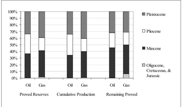
Siliciclastic deposits of the Miocene are currently the most productive unit in the northern Gulf of Mexico’s (GOM) stratigraphic column. For the central part of GOM, Miocene deposits account for 40% of all hydrocarbon proved-reserves and more than 40% of all remaining proved reserves (Figure 1). Remaining proved reserves are the quantities of proved reserves currently estimated to be recoverable. Estimates of remaining proved reserves equal proved reserves minus cumulative production (Crawford et al., 2002). 0% 10% 20% 30% 40% 50% 60% 70% 80% 90% 100%
Oil Gas Oil Gas Oil Gas
Pleistocene Pliocene Miocene Oligocene, Cretaceous, & Jurassic
Proved Reserves Cumulative Production Remaining Proved
The N-sand interval is typical of productive sands throughout the northern Gulf of Mexico (Shelby, 1988). It is proposed to conduct this study for the N-sand’s characteristic wide spatial distribution across the study area. Hydrocarbon production from this interval was reported from adjacent fields, Lighthouse Point, Mound Point and south Marsh block 236, to the fields of Tiger Shoal and Vermilion 50 of the South Marsh Island exploration area (Shelby, 1988). Earlier production within the N-sand interval was mainly restricted to structural closures associated with growth faulting. However, production from stratigraphic traps was also reported from the Upper Miocene deposits (Ray and Pearcy, 1988).
Seni (1997) believes that plays based mainly on structural reservoirs are of limited exploration use in mature areas, emphasizing that depositional/stratigraphic reservoirs remain a robust attribute, and they allow possibilities for predicting reservoirs in lightly drilled areas. Recently, Hentz and Zeng (2003) indicated that there are significant untapped hydrocarbon accumulations in nonstructural traps within the Miocene third-order lowstand systems tracts of the Tiger Shoal and Vermilion 50 fields. Accordingly, the use of N-sand interval provides a basis for the development of new hydrocarbon reserves both within the study area and in other mature and unexplored Miocene strata of the northern Gulf of Mexico shelf province.
1.4 Objectives of the study
The major objective of this study is to investigate the use of multivariate seismic attributes in order to obtain better spatial estimates of key reservoir properties of the N-sand interval of Tiger Shoal and Vermilion 50. These properties include: gross thickness, average gross effective porosity, net thickness, sand volume fraction and net reservoir porosity thickness product. In order to accomplish our main objective, the following specific objectives are to be met:
- Conduct structural and stratigraphic interpretation of the N-sand interval using 3D seismic and well log data.
- Generate multivariate attributes using multivariate statistical methods.
- Provide a general workflow for use in similar reservoir localities.
- Predict and map the lateral variations of reservoir properties using collocated cokriging.
1.5 Location of the study area
The study area lays on the outer shelf off the Louisiana shore line in northern central Gulf of Mexico (Figure 2). It is located to the south of Marsh Island between 29º 15` to 29º 38` (N) and 91º 49` to 92º 17` (W). Water depths in the region range from a few feet to 20 ft.
1.6 Data base
The data base consists of 3D seismic and well data. The seismic data is from to the federal lease OCS 310 located to the south of central Louisiana shore lines. The data were poststack time migrated. CDP spacing is equal to 112.61 by 109.83 ft. The sampling rate of the seismic data is 2 ms. The deepest imaged time is 6.0 seconds of two-way travel time (TWTT). A subset of this data base is included in this study. It represented a seismic coverage of approximately 246.5 km2, which is bounded between 1081 to 1432 in-lines and 152 to 802 cross-lines (Figure 3).
Well data consists of logs from 42 wells. Each well is given a distinctive name composed of the block number and the well number. For example, well number 4 of block 30 is named as 30-4. These wells are essentially restricted to the producing fields of Tiger Shoal and Vermilion 50. The well data includes a variety of digital well logs, ranging from electric to full suite logged wells. In addition, the well data base includes 8 wells with paleontological data (30-4, 31-3, 31-1, 31-14, 210-95, 211-6, 217-15, and 231-2), and 10 with check-shot velocity surveys.
The seismic data was donated by Texaco and well log data are donated by Texaco and A2D Inc. Velocity surveys, deviation surveys, culture data of lease block grids, and well’s upper and down hole well coordinates are provided by the Mineral Management Services. Paleontological data is provided by Texaco and the Mineral Management Services (www.mms.gov).
Figure 2. Location of the study area. The seafloor is less than 20 ft deep and is just a few miles south of the coasts of Louisiana. Area shaded in red denotes the portion of the seismic data used in this study (after Zeng et al., 2001).
8
Figure 3. Seismic basemap, limits of the area of interest (shown in blue border line), lease blocks and wells of Vermilion 50 (left) and Tiger Shoal fields (right).
CHAPTER II BACKGROUND 2.1 Seismic attribute technology
2.1.1 Introduction
Reservoir characterization is a systematic process for quantitatively describing reservoir properties. Usually, this process requires a multidisciplinary approach that integrates a wide array of data of various scales and sources.
The traditional function for using seismic data to reservoir seismology is mainly restricted to structural applications. However, recent advances in seismic technology have opened new doors for nontraditional uses of seismic data. The increasing demand for using seismic data as a predictive tool for the estimation of reservoir properties is mainly attributed to the advent of seismic attributes technology.
The general definition of seismic attributes defines any piece of information derived from seismic data as a seismic attribute. These attributes are function of some numerical measures of characteristics of the seismic data (Hart, 1999). Taner (2001) extended this definition to incorporate all possible information without any preference to their origin, “all the information obtained from seismic data, either by direct measurements or by logical or experience-based reasoning”.
Until early 1960’s, the use and the interpretation of seismic reflection data was largely a matter of mapping events and converting these events into depth maps to determine the geological structure of the subsurface (Barnes, 2001). Advances in the field of electronics and computing allowed the computation of seismic attributes, mostly derived from the basic seismic measurements of time, amplitude, frequency and attenuation (Brown, 1996). Figure 4 shows a general classification of the main seismic attributes derived from post-stack seismic data.
Seismic attributes can be divided into volume-based seismic attributes and map-based seismic attributes. Map-map-based attributes are considered as a major tool for a
detailed reservoir-level analysis (Brown, 2001) offering superior resolution and computational efficiency (Barnes, 2001). Not only had this shifted the interest in exploration seismology from a qualitative tool into a pure quantitative tool but also it shifted the scale of investigation from wide basin-scale studies into more detailed reservoir-scale studies.
Figure 4. The various types of post-stack seismic attributes derived from the basic seismic information of time, amplitude, frequency, and attenuation. The window can be a constant time interval, a constant interval hung from one horizon, or the interval between two horizons or depth (after Brown 2001).
Seismic Data
Amplitude
Time Frequency Attenuation
Horizon Time Isochron Trend Residual Dip Azimuth Difference Edge Illumination Cosine Phase Curvature Roughness Window Coherency Continuity Semblance Covariance Peak-Trough Difference Dip Max Correlation Azimuth Max Correlation
Signal-To-Noise Ratio Parallel Bed Indicator Chaotic Bed Indicator Trace Difference Horizon Reflection Amplitude Composite Amplitude Relative Impedance Reflection Strength Amplitude Ratio Normalized Amplitude Window Sum of Magnitude Total Energy Average Magnitude Average Energy Average Reflection RMS Amplitude
Average Peak Amplitude Variance of Amplitude Threshold Amplitude Maximum Amplitude Max. Negative Amplitude Peak-Trough Difference Energy Half-Time Slope Reflection Strength Slope At Half Energy Ratio Positive-To-Negative
Horizon
Instantaneous Frequency Response Frequency Weighted Inst. Freq. Time Derivative Freq.
Window
Average Inst. Freq. Reflection Width RMS Inst. Freq. No. Of Zero Crossings Peak Spectral Frequency Dominant Frequency Inst. Q Factor Slope Spectral Freq.
Slope Inst. Freq.
Hybrid Attributes
Arc Length Wave Shape Loop Area
2.1.2 The use of seismic attributes to predict reservoir properties, a quantitative interpretation approach
The famous “bright spot” technology of the late 1960’s and early 1970’s is one of the earliest direct applications of a seismic attribute to predict reservoir properties (Barnes, 1999). Ever since, the use of seismic attributes in reservoir characterization has drawn substantial interest because it provides better insight into the internal geological characteristics of a reservoir and its derived properties.
The two primary sources of data in reservoir characterization are well and seismic data. The integration of these two data inputs has been a consistent aim in reservoir characterization studies. Owing to the dense coverage of seismic data, seismic attributes can help to interpolate between sparse well data if it is possible to build a correlation between these two data types.
In a reservoir characterization seismic attribute study, an attempt is made to establish a statistically acceptable correlation between one or a group of seismic attributes with well log measured reservoir properties. A correlation, if found, can be used to predict the behavior and the distribution of the modeled reservoir property in areas outside well control (Schultz et al., 1994; Russell et al., 1997; Hart, 1999). Several methods are available for finding the transform that best predicts the targeted reservoir property. Methods of linear and non-linear regression, geostatistics and neural networks are among popular approaches (Russell et al., 1997; Hirsche et al., 1997; Kalkomey, 1997; Gastaldi et al., 1997).
In some situations, however, correlations between seismic attributes and reservoir properties can be misleading. Spurious correlations, as apparent correlations between uncorrelated variables, can lead to erroneous predictions. Kalkomey (1997) and Hirsche et al. (1998) showed that the probability of observing spurious correlations can be quite large if the number of well measurements is small or the number of attributes is large. Russell et al. (1997) stated that extra caution should be exercised when using more than one attribute and that there is an optimum number that should not be exceeded.