Harvard University
Harvard University Biostatistics Working Paper Series
Year Paper
Model Averaged Double Robust Estimation
Matthew Cefalu∗ Francesca Dominici† Nils D. Arvold MD‡ Giovanni Parmigiani∗∗
∗Harvard School of Public Health, [email protected] †Harvard School of Public Health
‡Partners, [email protected]
∗∗Dana-Farber Cancer Institute and Harvard School of Public Health
This working paper is hosted by The Berkeley Electronic Press (bepress) and may not be commer-cially reproduced without the permission of the copyright holder.
http://biostats.bepress.com/harvardbiostat/paper149 Copyright c2016 by the authors.
Model Averaged Double Robust Estimation
Matthew Cefalu, Francesca Dominici, Nils D. Arvold MD, and Giovanni Parmigiani
Abstract
Existing methods in causal inference do not account for the uncertainty in the selection of confounders. We propose a new class of estimators for the average causal effect, the model averaged double robust estimators, that formally account for model uncertainty in both the propensity score and outcome model through the use of Bayesian model averaging. These estimators build on the desirable double robustness property by only requiring the true propensity score model or the true outcome model be within a specified class of models to maintain consis-tency. We provide asymptotic results and conduct a large scale simulation study that indicates the model averaged double robust estimator has better finite sample behavior than the usual double robust estimator.
Model averaged double robust estimation
Matthew Cefalu1, Francesca Dominici2, Nils Arvold3, and Giovanni Parmigiani2,3 1 RAND Corporation
2 Harvard T.H. Chan School of Public Health 3 St. Luke’s Radiation Oncology Associates
4 Dana-Farber Cancer Institute
Corresponding author: [email protected] September 2, 2016
Abstract
Researchers estimating causal effects are increasingly challenged with decisions on how to best control for a potentially high-dimensional set of confounders. Typically, a single propensity score model is chosen and used to adjust for confounding, while the uncertainty surrounding which covariates to include into the propensity score model is often ignored, and failure to include even one important confounder will results in bias. We propose a practical and generalizable approach that overcomes the limitations described above through the use of model averaging. We develop and evaluate this approach in the context of double robust estimation. More specifically, we introduce the model averaged double robust (MA-DR) estimators, which account for model uncertainty in both the propensity score and outcome model through the use of model averaging. The MA-DR estimators are defined as weighted averages of double robust estimators, where each double robust estimator corresponds to a specific choice of the outcome model and the propensity score model. The MA-DR estimators extend the desirable double robustness property by achieving consistency under the much weaker assumption that either the true propensity score model or the true outcome model be within a specified, possibly large, class of models. Using simulation studies, we also assessed small sample properties, and found that MA-DR estimators can reduce mean squared error substantially, particularly when the set of potential confounders is large relative to the sample size. We apply the methodology to estimate the average causal effect of temozolomide plus radiotherapy versus radiotherapy alone on one-year survival in a cohort of 1887 Medicare enrollees who were diagnosed
1
Introduction
Methods for causal inference are predicated on knowledge of the covariates necessary to satisfy the no
unmeasured confounding assumption, but the exact set of covariates needed to control confounding is
rarely known. With the growing use of causal inference methods in large observational studies, such as
administrative databases used in comparative effectiveness research, the set of potential confounders can be
quite large. Practical tools that acknowledge uncertainty in confounder selection and are robust to model
misspecification are imperative for correct estimation of the average causal effect (Vansteelandt et al., 2012;
Wang et al., 2012; Zigler and Dominici, 2014; Wang et al., 2015). Extracting the minimal and necessary
set of covariates for confounding adjustment in the final data analysis becomes more difficult as the set of
potential confounders grows. Failure to adjust for even one important confounder may lead to a biased
estimate of the causal effect of interest.
Several attempts have been made to develop methods for confounder selection in causal inference
(Joffe et al., 2004; Brookhart et al., 2006; Schneeweiss et al., 2009; Wang et al., 2012; De Luna et al.,
2011; Gruber and van der Laan, 2012; Shahar, 2013; Vansteelandt et al., 2012; VanderWeele and Shpitser,
2011; Wilson and Reich, 2014; Zigler and Dominici, 2014; Wang et al., 2015). Most of these authors
note that statistical methods to select confounders pose unique challenges, and methods designed for
prediction may not be directly applicable. Statistical methods to select potential confounders based on the
outcome model prioritize covariates strongly associated with the outcome, while variable selection based
on a treatment model prioritize covariates that are strongly associated with the treatment. Both these
approaches can result in inefficient and biased inferences because they can fail to identify the full set of
necessary confounders.
One set of methods for confounder selection builds on Bayesian model averaging (Wang et al., 2012,
2015). These authors propose an approach, called Bayesian adjustment for confounding (BAC), to estimate
the effect of a continuous exposure (or treatment) on an outcome, while accounting for the uncertainty
in the choice of confounders. Their approach is based on specifying two models: (1) the outcome as a
function of the exposure and the potential confounders; and (2) the exposure as a function of the potential
confounders. They assume a priori that if a covariate is highly predictive of the exposure then the same
Zigler and Dominici (2014) use similar ideas in the context of a propensity score analysis for binary
treatment (Rosenbaum and Rubin, 1983). They propose a Bayesian model averaging approach that adjusts
for confounding by using the propensity score as a linear predictor in an outcome model. To handle the
so-called “feedback” issue (McCandless et al., 2010; Zigler et al., 2013), the proposed method forces variables
that are included in the propensity score model to also be included as linear predictors in the outcome
model.
Although these methods have, in our view, formulated the problem of confounder selection soundly and
proposed workable solutions, they rely on parametric assumptions to estimate causal effects. For example,
the methods of Wang et al. (2012), Zigler and Dominici (2014), and Wang et al. (2015) specify a sampling
distribution for the outcome model and rely on covariate adjustment through a linear predictor in an
outcome model. Also, these methods do not provide an easily generalizable procedure for extending widely
used non-Bayesian causal inference methodologies, including useful nonparametric and semi-parametric
methodologies that rely on on selection of confounders. The goal of this paper is to provide a practical
and generalizable strategy for robustifying a broad range of causal inference methodologies with regard
to model choice. Our approach borrows and simplifies Bayesian ideas, but strays from a fully coherent
Bayesian specification. We wish to leverage existing non-Bayesian tools to mitigate the negative effects of
overlooking the uncertainity due to model selection.
We are particularly interested in applications presenting a large number of potential confounders relative
to the sample size. In this setting, uncertainty on confounder selection is especially important. In a setting
where we estimate a regression coefficient, we often make several assumptions regarding the sampling
distribution of the outcome, the functional form relating the covariates to the outcome, and which covariates
we include into the the regression model. In causal inference, it is common to assume a model for the
propensity score, thus leading to uncertainty regarding which covariates the analyst decides to include into
the propensity score model, including the functional form.
We develop and evaluate our model averaging approach focusing on the double robust estimator. The
result is a newly proposed family of estimators, the model averaged double robust estimators, formally
accounting for model uncertainty through the use of model averaging while extending the desirable double
model and propensity score model, where each of these models can include a different subset of all the
potential confounders. We compute model-specific double robust estimators as a function of the outcome
model and a propensity score model, and then average over these using weights that are motivated by
posterior model probabilities, though not always interpretable as such. We introduce a prior distribution
on the model space that (1) a priori links the outcome and the propensity score model, (2) assigns higher
prior probabilities to propensity score models that include necessary confounders (i.e. covariates that are
associated with both the treatment and the outcome), and (3) assigns low prior probability to propensity
score models that include covariates that are only associated with the treatment. By conducting several
simulation studies with varying sample sizes, number of potential confounders, and strength of confounding
bias, we show that by specifying this prior distribution, and using the resulting posterior model probabilities
as weights in a model averaged double robust estimate, we substantially increase efficiency.
In Section 2, we introduce a general framework for model averaging in causal inference and model
aver-aged double robust estimation. In Section 3, we provide asymptotic results about our proposed estimators.
In Section 4, we provide a simulation study that illustrates the finite sample performance of model averaged
double robust estimators. In Section 5, we apply the model averaged double robust estimator to estimate
the comparative effectiveness of temazolomide on 1-year survival after diagnosis with glioblastoma.
2
Methods
2.1 Notation and General Approach
To facilitate the presentation of our framework for model averaging in causal inference, consider first the
estimation of the causal effect ∆ of a binary treatment using an inverse probability of treatment weighted
estimator (IPW). Instead of selecting a single propensity score model, let’s consider the class of propensity
score modelsMthat includes logistic and probit regression models with all possible subsets of the potential confounders as linear predictors. If, within class M, we choose the ith model Mi ∈ Mfor analysis, then
the resulting estimator of the causal effect will inherit properties that depend on that choice, a fact we
record via the notation ∆(b Mi). To robustify the estimation process with respect to choice of model, a
b
∆M A= X
i:Mi∈M
wi∆(b Mi), (1)
wherewi ∈[0,1] is the weight assigned to modelMi and Piwi = 1.
Beyond the IPW example, this defines a general class of model averaged estimators built using any
desired combination of estimated weights and estimated model-specific causal effects. In Section 3, we will
show that, under standard regularity conditions, if the underlying causal estimate is consistent under the
true modelMtrue, then the weighted version will also be consistent, as long as the true model belongs to
the model classMand the weights converge to a degenearte distribution on the true model. This provides
the general motivation for the approach. In this paper, we investigate it specifically for double robust
estimation.
Looking ahead, the implementation of a model averaged estimate requires a strategy for assigning
weights wi to models. The focus of this paper will be on the case where the weights wi corresponds to
the posterior model probabilities, but one could consider model weights derived from other criteria such
as minimizing mean squared error (Longford, 2006).
2.2 Double robust estimator
LetY(x) be the potential outcome that would have been observed under treatmentX=x,x∈ {0,1}. The observed outcomeY is related to the potential outcomesY(x) byY = I(X=x)Y(x), where I(X=x) is the
indicator thatX=x. Consider ap-dimensional set of potential confoundersC, and assume strong ignorable
treatment assignment (Rosenbaum and Rubin, 1983), so that (Y(0), Y(1)) ⊥⊥ X|C. Let (Yh, Xh, Ch) be
independent observations forh= 1, ..., n. We are interested in estimating the average causal effect:
∆ =E[Y(1)−Y(0)] =E[E(Y|X= 1, C)−E(Y|X = 0, C)]. (2)
Given a model for the propensity score, P(X = 1|C) = e(C), and models for the outcome under each
robust (∆bDR) estimator as: b ∆DR = 1 n n X h=1 YhXh−(Xh−beh)mb1h b eh −Yh(1−Xh) + (Xh−ebh)mb0h 1−beh , (3)
wheremb1h,mb0h, and beh are the estimates ofm1(C),m0(C), ande(C) for individualh (Bang and Robins,
2005). The double robust estimator is regarded as semi-parametric because the estimation procedure only
depends on the specification of the conditional means P(X = 1|C), E(Y|X = 1, C), and E(Y|X = 0, C) and does not rely on a fully parametric specification of the models.
The propensity score model and the outcome models can be selected in any number of ways. A
researcher may rely on expert knowledge to decide both the functional form and the confounders to
include in each model, or may rely on a model selection procedure that chooses the best model from
a set of candidate models. For the remainder of this paper, we will refer to ∆bM SDR as the “model selected
double robust estimate” in which both the propensity score and the outcome models have been selected
independently using BIC.
2.3 A model averaged double robust estimator
Next we apply the model averaging outlined in Section 2.1 to the double robust estimator. We chose to
consider the double robust estimator because of its wide use and strong asymptotic properties. Also, it
will highlight the flexibility of our approach because it relies on the specification of multiple models.
Let Mps = nMps 1 ,M ps 2 , ...,M ps Mps o , M0 = M0 1,M02, ...,M0M0 , and M 1 = M1 1,M12, ...,M1M1 be
finite collections of models for the observed data likelihoods p(X = 1|C), p(Y|X = 0, C), and p(Y|X = 1, C), respectively. In this paper, the models can vary depending on inclusion of potential confounders in
linear predictors. Similar approaches could consider distributional assumptions, link functions, specification
of the functional form of the predictors (e.g. inclusion of interactions) and more. Let Mom =M1× M0
denote all combinations of models in M1 and M0. Further, define
b
∆DRij as the double robust estimate
corresponding to the models Mpsi and Mom
estimate ∆bM ADR as a weighted average of model specific double robust estimates ∆bDRij , that is:
b
∆M ADR =X
ij
wij∆bDRij . (4)
Herewij = P(Mpsi ,Momj |D) is the joint (approximate) posterior probability of modelsM ps
i andMomj and
b
∆DRij is the double robust estimate that uses the plug in estimates of m1b h, m0b h, andebh corresponding to
Mpsi and Mom
j . The estimation of the weightswij is performed independently of the estimation of∆bDRij .
Posterior model probabilities depend on the likelihoods of the models in the model space, along with
the prior distribution on the model space. The specification of the likelihood used in deriving the weights
plays no role (except through the conditional means) in the estimation of the model specific effects ∆bDRij ,
which remains semiparametric and robust to higher order moments of the true data generating mechanism.
2.4 Priors on the model space
2.4.1 Uniform prior on the model space
To derive weights, we specify a prior distribution on the model class, and compute approximate posterior
probabilities. The simplest choice is to assume that all models are independent and equally likely a priori,
which we will refer to as a uniform prior on the model space. This implies that the prior odds of each
model is 1, and that the prior distribution on the propensity score model class is independent of the prior
distribution on the outcome model class. Because of the independence assumption, the posterior model
probabilities factor as P(Mpsi ,Mom j |D) = P(M ps i |D)P(Momj |D). Therefore, P(M ps i |D) and P(Momj |D)
can be computed separately, which substantially simplifies the computation.
The resulting posterior distribution assigns high weights to propensity score models that include Cs
strongly associated with X and does not consider relationships with Y. The current literature in causal
inference suggests that inclusion of covariates that are only related to the treatment into a propensity score
model adds to the variance of the resulting estimator (Rubin et al., 1997; Hahn, 2004; Brookhart et al.,
2.4.2 Dependent prior on the model space
In view of this consideration, efficiency can be gained through the use of a prior distribution on the
propensity score model space that favors inclusion of potential confounders that are associated with both
treatment and outcome, instead of predictors associated only with treatment (Rubin et al., 1997; Hahn,
2004; Brookhart et al., 2006; Wooldridge, 2009; Pearl, 2009; Groenwold et al., 2011; Vansteelandt et al.,
2012). With this goal in mind, we propose an alternative prior distribution on the model space that links
the propensity score model to the outcome model through prior model dependence. We assume that the
prior odds of including a potential confounder in the propensity score model given that it is included in
the outcome model is 1, and that the prior odds of including a potential confounder in the propensity
score model given that it is excluded from the outcome model is small. This dependence also implies that
the prior odds of including a potential confounder in the outcome model given that it is included in the
propensity score model is high.
Specifically, we assume that both Mps and Mom contain models with linear preditors comprising
potential confounders. We let Mpsi ⊂ Mom
j indicate that the terms in the linear predictor of M ps i are
a subset of those of Mom
j . Since Mom is the product space of M0 and M1, we evaluate the inclusion
relation above using the union of terms in the linear predictors from the corresponding models inM0 and
M1. To specify the prior, we choose a reference propensity score model Mps
1 such that M
ps
1 ⊂ Momj for
all j. Thus, Mps1 is either a null model or a model that includes the potential confounders that will be included in all models. We set the prior odds of propensity score modelMpsi to modelMps1 conditional on
the outcome modelMom j to be: P(Mpsi |Mom j ) P(Mps1 |Mom j ) = 1, ifMpsi ⊂ Mom j τ, otherwise , (5)
forτ ∈[0,1]. Lastly, we assume that the prior distribution on the outcome model space is uniform.
The choice of τ is important. First, τ = 1 corresponds to the uniform prior on the model space of the
previous section. Second, whenτ = 0, the prior model dependency given by (5) restricts the set of potential
Third, when τ is nonzero but smaller than 1, the prior dependency of (5) gives small weight a priori to
propensity score models including terms that are not included in the outcome model. Finally, whenτ >1,
the prior assigns small weights to outcome models including a larger set of covariates than that included
into the propensity score model. We generally avoid this choice, as terms that are predictive of the outcome
but not the treatment can still contribute to more efficient estimation of the causel effect.
2.5 Estimation of model weights
2.5.1 BIC approximation of posterior model probabilities
The posterior model probabilities, which are used as model weights in (4), are a function of the Bayes
factors and the choice of prior distribution on the model space. In general, the Bayes factor for
com-paring model Mi to model Mj is defined as Bij = p(D|Mi)/p(D|Mj), where D denotes the data
and p(D|Mi) = R
p(D|Mi, ηi)p(ηi|Mi)∂ηi is the integrated likelihood over all model-specific
parame-ters ηi within Mi. A simple transformation of the Bayes factors gives the posterior model probabilities,
P(Mi|D) =AiBi1/Pj:Mj∈MAjBj1, whereAi is the prior odds ofMi versus a reference modelM1.
Out-side of a few special cases, the Bayes factorBij will not have a closed form, and an approximation will be
necessary. A widely used approximation of Bayes factors is based on the Bayesian Information Criterion
(BIC) (Schwarz, 1978), which we adopt in this paper. Other information criteria can be used to derive
model weights, such as the Akaike Information Criteria (AIC) (Akaike, 1998). See Yang (2003, 2005) for a
discussion of the relative merits of using AIC versus BIC in model averaging. As the number of models in
Mincreases, evaluating the Bayes’ factor for every model becomes computationally infeasible. Instead, we
can use a Markov chain Monte Carlo algorithm such as MC3 (Madigan et al., 1995) to search the model
space.
2.5.2 Two-stage posterior weights
Model weights based on the prior given in (5) still have the potential limitation that the resulting posterior
model probabilities will favor outcome models that include potential confounders that are only associated
with the treatment. This can result in a loss of efficiency. Specifically, the prior was described with the goal
both the treatment and the outcome. However, the prior can have a different effect: potential confounders
strongly associated with only treatment are included in both the propensity score and outcome models.
As previously discussed, inclusion of such covariates reduces efficiency.
As an alternative, we propose a two-stage approach for calculating the model weights motivated by
De Luna et al. (2011), who suggested to first identify the covariates associated with the outcome, and then
identify the covariates associated with the treatment among those associated with the outcome. First, they
suggest to find a reduced covariate vector, CY, such that p(Y0, Y1|C) =p(Y0, Y1|CY) holds. Second,CY is
further reduced intoZ such that p(X = 1|CY) =p(X = 1|Z) holds. They show that the covariate setsCY
and Z are sufficient for the identification of the average causal effect, and that using Z in nonparametric
estimation improves efficiency.
With this in mind, we propose the following two-stage approach for calculating model weights:
1. Compute the marginal posterior probability qj of thejth outcome model, assuming a uniform prior
and without considering the propensity score model;
2. Compute the conditional posterior probability P(Mpsi |Mom
j ,D) of the ith propensity score model,
conditional on knowing the terms included in the linear predictor of the outcome model, using prior
model dependence given by (5);
3. Multiply the estimates from Stage 1 and 2 to calculate model weightw∗ij =qjP(Mpsi |Momj ,D).
The model weights under this two-stage approach can be calculated easily because they are a
transfor-mation of the model probabilities assuming a uniform prior on the model space. The difference between
the two-stage model weightswij∗ and the proper posterior model probabilities under the same prior is that
the two-stage approach restricts the marginal outcome model weights to be equal to the marginal posterior
outcome model probabilities under a uniform prior on the model space. Thus the qj in Stage 1 of the
two-stage method does not correspond to the marginal posterior P(Mom
j |D) under the dependent prior,
while the estimation of P(Mpsi |Mom
j ,D) in Stage 2 does correspond to the conditional posterior under this
3
Asymptotic properties
For a general ∆bM A defined in (1), we show that, if the underlying causal estimate is consistent under the
true model Mtrue, and the true model belongs to the model classM, then the model averaged estimator
will also be consistent:
Theorem 1 Let Mbe a finite collection of models. Assume: (1) M contains the true model,Mtrue, (2)
the regularity conditions necessary for ∆btrue
p
→ ∆, are met and (3) ∆(b Mi) is bounded in probability for
alli. Then ∆bM A p→∆.
For the model averaged double robust estimator, we show that if the posterior model probabilities
are converging to the true models and if the true propensity score model OR the true outcome model is
contained in the corresponding model space, then ∆bM ADR is consistent for the average causal effect (2). We
regard this as an important relaxation of the robustness properties of the double robust estimator, as we
only need the true models to be included in a potentially large collection of models.
Theorem 2 Assume conditions (2) and (3) of Theorem 1. LetMom, Mps be collections of models. If:
(1) Mom contains the true models, Mom
1 , for both E(Y|X = 1, C) and E(Y|X = 0, C), and p•1 =
P iP(M ps i ,Mom1 |D) p →1
or (2) Mps contains the true model, Mps
1 , for P(X= 1|C), andp1•= P jP(M ps 1 ,Momj |D) p →1 Then, ∆bM ADR p →∆
For proofs, see Web Appendix B.
We chose to specify conditions of Theorem 2 in relation to the true data generating models to be
consistent with the literature on double robustness. However, the same conclusion could be reached
using weaker conditions, as long as the model space includes a model pair that produces a consistent effect
estimate. One such example may be a model that is sufficient for controlling confounding (Greenland et al.,
1999; De Luna et al., 2011; Vansteelandt et al., 2012). To see this, consider Lemma 2. First, we note that
the true propensity model is not necessary to maintain the consistency of the doubly robust estimator.
Instead, we only require a propensity score model, Mps1 , such that be(M1ps) = Pb(X = 1|C,M
ps
1 )
p
P(X = 1|C,Mpstrue). Assume that the model class Mps contains this consistent model, Mps 1 . If p1• = P jP(M ps 1 ,Momj |D) p →1, then ∆bM ADR p
→∆. A similar argument can be made with regard to the outcome
model, to relax Theorem 2.
4
Simulation study
4.1 Setup
In this section, we illustrate the finite sample behavior of ∆bM ADR relative to alternatives. We consider:
(1) the double robust estimate using model selection separately for the propensity score and the outcome
model (∆bM SDR); (2) the model averaged double robust estimate that assumes the prior model dependence
of (5) with τ ∈ {1,0.1,0.01,0} (∆bM ADR); (3) the model averaged double robust estimate that uses the
two-stage approach for calculating model weights withτ ∈ {1,0.1,0.01,0}(∆bM ADR−II); and (4) the collaborative
double robust targeted maximum likelihood estimator (van der Laan and Gruber, 2010; Gruber and van der
Laan, 2010) (∆bC−T M LE). See Table 1 for a description of the estimators considered in these simulations.
A description of the C-TMLE algorithm can be found in Web Appendix C.
We generate the data as follows: (1)C1, ..., Cp iid
∼N(0,1); (2)X ∼Bernoulli(p= expit(Cαps)); and (3)
Y ∼N(βX+Cαom, σ2). We consider different values of the unknown parametersαps andαom to capture different levels of confounding, and vary both the sample sizenand the number of potential confoundersp.
In all simulations, β = 1, implying that ∆ = 1. The simulation scenarios are defined in Table 2. We
restrict Mps and Mom to only include linear combinations of the p potential confounders so that there
are 2p models for both the propensity score and the outcome. The number of models in each class may be
large depending on the number of potential confounders.
4.2 Results for n= 200, p= 5, and σ2 = 4
The simulations of this section are intended to explore whether, even in simple scenarios with only 5
covariates and strong signals (i.e. αom and αps), model averaging has benefits over model selection. We
consider as gold standard the results obtained using the true outcome model. For each of the simulation
interval coverage, and relative efficiency compared to the gold standard. All estimators show very small
bias compared to the true ∆ = 1. The proposed model averaged estimators tend to have smaller standard
errors than their model selected counterparts.
Model averaging assuming prior model independence,∆bM ADR withτ = 1, is comparable to model selection
across all four simulation scenarios, with only negligible gains in efficiency. This suggests that even a
relatively unsophisticated implementation of model averaging to account for model uncertainty may do no
worse than model selection. The estimators assuming prior model dependence have standard errors that
are generally smaller than that of ∆bM SDR.
Scenario 3 is worth further discussion as it illustrates a substantial difference in the relative performance
of the model averaged estimators. Here onlyC1 andC2 are confounders, whileC3,C4, andC5 are strongly
associated with the exposure only (i.e. they are instruments). The model averaged estimators (except
b
∆M ADR−II withτ = 0) have relative efficiencies less than 0.6, ∆bC−T M LE has relative efficiency of 0.74, and b
∆M ADR−II with τ = 0 has relative efficiency of 0.98. Here, all potential confounders are linear in both
the propensity score and the outcome model, yet model averaging can reduce the variance of the double
robust estimator dramatically if we assume prior model dependence and use the two-stage approach for
estimating the model weights with τ = 0. Also, note that using model selection on the propensity score
model independently of the outcome model will tend to choose propensity score models that include C3,
C4, and C5. As these three potential confounders are unrelated to the outcome, their inclusion in the
propensity score model only adds to the variance of the model selected estimator.
To better characterize the relative performance of the model averaged estimates, Table 5 provides the
mean posterior inclusion probability of the covariates in the outcome model and in the propensity score
model. First, considering ∆bM ADR, we observe that as τ goes to zero, the posterior concentrates on outcome
models that include C3, C4, and C5. This is an unintended consequence of the prior model dependence,
which was designed in the hope that it would excludethese instruments from the propensity score model
instead ofincludingthem in the outcome model. Inclusion of instruments in the outcome model can inflate
the variance of the estimated causal effect. Next observe that, for ∆bM ADR−II where we use the two-stage
procedure for calculating the model weights, the inclusion probabilities for the instruments are 0.12 when
three covariates are strong predictors of treatment and the signal overwhelms the prior. Only very small
choices of τ will influence the posterior inclusion probabilities in this scenario. The estimator ∆bM ADR−II
with τ = 0 has smaller variance than the other estimators because it effectively down weights propensity
score models that includeC3,C4, andC5.
These simulations demonstrate that the model averaged double robust estimator with a two-stage
dependent prior withτ = 0 performs nearly as well as the gold standard in many of the scenarios considered
and performs substantially better than all of the competitors in Scenario 3.
4.3 Results for n= 200, p= 100, and σ2 = 1
An important motivation for model averaging approaches is their applicability to analyses with a large
sets of potential confounders, where substantive knowledge can be of limited help in specifying models,
and where several models receive support from the data. Rather than ignoring model uncertainty, we can
leverage information from the data to reduce the set of potential confounders to a manageable size through
the use of model averaging and a carefully chosen prior distribution on the model space.
To illustrate, we now consider a set of potential confounders that is half the size of the number of
observations (p= 100 andn= 200). The model space of the propensity score alone has 2100= 1.27∗1030 potential models while the joint model space has 2200 models. It is impossible to enumerate a set of models
this large, and evaluating balance within even a small set of these models can be challenging. Instead, our
prior distribution on the model space prioritizes propensity score and outcome models that share potential
confounders. We then search for these models stochastically using a Markov chain Monte Carlo model
composition (MC3) (Madigan et al., 1995). For computational efficiency, we focus on∆bM ADR−dII withτ = 0
and do not consider any of the other model averaged estimators with the dependent prior.
Overall, the prior model dependence given by (5) with τ = 0 in the two-stage approach appears to
be very effective at reducing the propensity score model space. This reduction increases both statistical
and computational efficiency, while promoting inclusion of the correct confounders. By searching a smaller
space of models, we may also be more likely to find regions of the model space with higher posterior
probabilities. The resulting estimator ∆bM ADR−dII dramatically improves efficiency when compared with
Specifically, we repeated the simulations from Section 4.2, but generate a total of p = 100 potential
confounders and reduced σ2 to be 1. We consider the same four scenarios given in Table 2, but include
an additional 95 covariates that are unrelated to both the treatment and outcome. In addition to these
simulations, we consider one additional scenario (Scenario 5) to mimic a situation where the sets of
co-variates associated with only the outcome or only the exposure are large, but the overlap between these
two sets is small. Specifically, we generate 20 covariates only related to the outcome, 10 related to both
the outcome and the exposure (and hence confounders), 20 covariates related only to the exposure, and 50
additional noise covariates. This adds to a total of p = 100 potential confounders, while the sample size
remainsn= 200. The strength of the relationships between the potential confounders, the outcome, and
the exposure were randomly generated. Details can be found in Web Appendix D.
Table 4 provides the mean, standard error, bootstrapped 95% confidence interval coverage, and relative
efficiency compared to the gold standard for each simulation scenario defined in Table 2 but withp= 100.
The superiority of ∆bM ADR−dII compared to alternatives is even more striking when p = 100. Relative
efficiencie is above 0.80 for all five scenarios, while the other estimators suffer from a severe loss of efficiency.
The model averaged double robust estimator assuming prior model independence continues to have smaller
standard error when compared with model selection. However, the differences in efficiency between the
two are no longer negligible, with ∆bM ADR with τ = 1 having less variance.
The gains in efficiency of the model averaged double robust estimator over the model selected estimator
illustrates that withn= 200 observations, the sample size is not large enough to reflect the fact that model
selection and model averaging are asymptotically equivalent. With∆bM ADR−dII andτ = 0 specifically, the use
of the two-stage approach for calculating model weights is effective at identifying the models that include
potential confounders that are associated with both the treatment and the outcome. This feature becomes
increasingly important as the set of potential confounders increases. In Scenario 5, there are p = 100
potential confounders but only 10 are actual confounders, while 30 are related to only the exposure.
Therefore, the gains in efficiency observed in Scenario 5 are likely due to placing higher weights on the
propensity score models that include the 10 confounders, as opposed to selecting a propensity score model
that includes all 30 potential confounders only associated with the exposure.
by the confounders that are selected, and the data generating model is included in the class. More work
is needed to determine the relative merits of the model averaged double robust estimators when these
assumptions are relaxed. With regard to the first, suppose that the set of confounders was known, but the
exact functional forms relating the confounders to the outcome and treatment are unknown. The model
averaged double robust estimator can be used in this setting as well; the model classes would contain
various specifications of how the confounders appear in the models (e.g. interactions, polynomials, splines,
etc.). In this setting, we expect the model averaged double robust estimator to perform well provided that
the model classes are flexible enough to capture important features of the data.
5
Comparative effectiveness of temozolomide for treating glioblastoma
The SEER linked Medicare database was used to construct a cohort of 1887 Medicare beneficiaries who
were diagnosed with glioblastoma from June 2005 to December 2009 to compare the effectiveness of
temo-zolomide plus radiotherapy (X = 1) vs. radiotherapy alone (X = 0) for lowering the probability of
death within 1 year of diagnosis. For more background on glioblastoma and temozolomide see Arvold and
Reardon (2014) and Arvold et al. (2014).
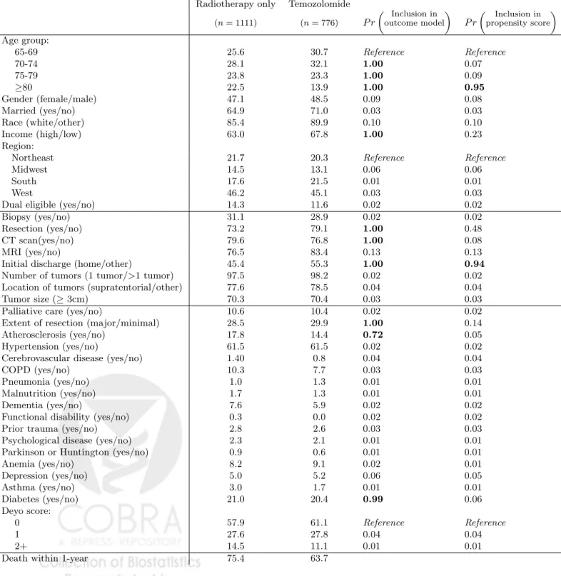
Table 6 summarizes 33 baseline characteristics of patients who were treated with temozolomide plus
radiotherapy (n= 776) and those who were treated with radiotherapy alone (n= 1111). Younger patients
were more likely and older patients were less likely to received temozolomide. Other differences in baseline
characteristics between the treatment groups include the use of diagnostic tests (MRI and CT scan), the
extent of resection, income, race, and the patient comorbidities atherosclerosis and COPD as measured by
the Hierarchical Condition Categories (Pope et al., 2004). The unadjusted rate of death within 1 year of
diagnosis is 11.7% (7.6-16.0%) lower in the patients receiving temozolomide plus radiotherapy compared
to radiotherapy alone (63.7% versus 75.4%).
We estimate the average causal effect of temozolomide plus radiotherapy (vs. radiotherapy alone) on the
probability of death within 1 year of diagnosis using the model averaged double robust estimator assuming
prior model dependence defined by (5) withτ = 0 and using the two stage approach for calculating model
weights. We specify logistic regression models for both the propensity score model and outcome model. The
effects. The outcome model class contains logistic regressions that include the treatment and all possible
subsets of the covariates as main effects. With 33 covariates, the joint model space has 22∗33 = 7.4∗1014 possible models. MCMC chains were run for 10,000 iterations. We estimate the rate of death within 1 year
of diagnosis is 6.7% (2.4-10.7%) lower in the patients receiving temozolomide using the model averaged
double robust estimator. This compares with the double robust estimator that includes all covariates in
both the outcome and propensity score models that estimates a 6.4% (2.5-10.4%) lower mortality rate
within 1 year of diagnosis for the patients receiving temozolomide. We also performed model selection,
where we selected the propensity score and outcome model independently using BIC, and estimated the
effect of temozolomide at 7.3% (3.5-11.1%). Notice that the 95% confidence intervals are slightly wider
for the model averaged double robust estimator. This is expected, as the model averaged double robust
estimator accounts for model uncertainty. As we will now discuss, the confidence intervals for the model
averaged double robust estimator are only slightly wider because there is very little uncertainty in the
selection of confounders in this example.
One benefit of utilizing model averaging is that the posterior probability of inclusion can be calculated
for each potential confounder. Included in Table 6 are posterior inclusion probabilities in both the
propen-sity score and outcome models. One can loosely interpret the probability of inclusion in the propenpropen-sity
score model as the probability of being a confounder because of the prior distribution and the two stage
method used for calculating the model weights. Note that the age category 80+ years has a posterior
inclusion probability in the propensity score model of 0.95, and the indicator of a home discharge after
diagnosis has a posterior inclusion probability of 0.94. These large inclusion probabilities suggest that
the data indicates that age and initial discharge location are related to both 1-year survival and receipt
of temozolomide; therefore, age and discharge type are important confounders. The only other patient
characteristic to have considerable posterior probability in the propensity score model is an indicator of
resection, with a probability of 0.48.
These results suggest that there are only a few important confounders of the relationship between
1-year survival and receipt of temozolomide. This is not completely unexpected, as glioblastoma patients
have poor prognosis and complications tend to arise from disease progression. This is reflected in the
receive treatment.
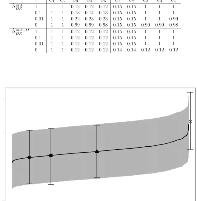
Figure 1 provides the model specific double robust estimators and corresponding 95% confidence
inter-vals for 1000 randomly chosen outcome models and 1000 randomly chosen propensity score models. The
unadjusted estimator of 11.7% (7.6-16.0%) is beyond the upper end of the distribution of the model specific
estimates, while the model averaged double robust estimator of 6.7% (2.4-10.7%) is near the lower end of
distribution. All of the model specific estimates are lower in magnitude than the unadjusted estimator,
suggesting that any choice of models leads to a more conservative estimate of the difference in 1-year
mor-tality when compared to the unadjusted estimator. The model averaged double robust estimator allows us
to incorporate this model uncertainty into our final estimator by taking a weighted average of these model
specific estimates. Figure 1 nicely provides a fully transparent illustration of the sensitivity of ˆ∆DR to the
choice of potential confounders in the outcome and propensity score models. We also see that the model
selected estimate is anti-conservative when compared to the model averaged estimate or the double robust
estimate that includes all of the covariates.
These results highlight the usefulness of the estimator at providing researchers with data-driven
indi-cations of the uncertainty surrounding the choice of confounders while returning consistent estimation of
the causal effect of interest.
6
Discussion
In this paper we present a model averaging framework that can be used to robustify any causal estimator
that depends on the specification of a model. We focused on the double robust estimator to highlight that
model averaging is possible in contexts not yet explored in causal inference. The model weights used in this
paper were derived from approximate posterior model probabilities, but one could consider weights derived
from other criteria (e.g. model weights based on the balance of covariates between treatment groups).
Studying the properties of alternate weights and the use of model averaging on other estimators in causal
inference is an exciting line of research.
Our results build on the most basic double robust estimator for the average causal effect. It has
been demonstrated elsewhere that this double robust estimator can be biased especially when some of
estimator have been proposed (Robins et al., 2007; Cao et al., 2009; Tan, 2010). We expect that results
similar to those presented here may hold for these other estimators. Additionally, the model averaged
double robust estimator does not assume that the confounders’ effect on the potential outcomes is the
same between treatment groups, as a model for the outcome under each treatment can be specified.
Our model averaged double robust estimator shares some similarities with the work of Han and Wang
(2013) who propose a method that allows the specification of multiple models for both the propensity score
and the outcome regression. One difference in the methods lies in how the models are combined to produce
the final estimator. We propose to take a weighted average of the model specific estimates, whereas Han
and Wang (2013) combine the models to produce a subject specific weight, wbi and define their estimator
as µb =P b
wiYi. While we propose a general procedure for model averaging in causal inference, it is not
immediately clear to us whether the method of Han and Wang (2013) extends to other estimators.
A central piece in the construction of a model averaged estimator is the prior placed on the space
of possible models. In this area there are opportunities to expand our work and potentially improve
it substantially. For example, while our prior guarantees consistency in asymptotics with fixed p and
increasing n, it would be interesting to investigate consistency when both p and n grow; in this setting
a uniform prior on the model space can lead to inconsistency and priors that penalize model complexity
may have better properties. The prior of (5) controls the prior probability of model combinations that
do not meet the restriction Mps ⊂ Mom through τ. However, model combinations that do not meet this
restriction have the same prior probability. This implies that, given an outcome model, the prior probability
of a propensity score model that includes all the potential confounders included in the outcome model plus
one additional potential confounder is the same as that of a propensity score model that includes all of
the potential confounders that were excluded from the outcome model. In other words there is no prior
penalization for complexity within these subspaces. In related work we have explored selecting priors that
achieve a good balance between confounding adjustment and model parsimony. See Wang et al. (2012,
2015).
Scott et al. (2010) investigate priors that control for multiplicities in Bayesian variable selection. They
stress that multiplicities are essential when one uses variable selection methods as exploratory tools whose
important ways: first, in our case, the final model and associated causal effect estimate are the main focus;
secondly we do not select, we average. Nonetheless multiplicity properties may be a desirable property for
a prior, achievable by allowing prior model probabilities to depend upon the data in an appropriate way.
Our prior does not automatically adjust for multiplicities in this sense.
Causal inference approaches are increasingly used to analyze large observational studies, such as
admin-istrative databases in comparative effectiveness research. In these applications, there seldom is a clear-cut
way of determining a priori the precise set of confounders of scientific relevance. At the same time,
im-provements in computing speed and parallelization are creating the opportunity for a more systematic
investigation of alternative specifications for confounding adjustment. In these settings, the proposed
model averaging strategy shows great promise as a data analysis tool to perform robust and consistent
7
Supplementary Materials
Web Appendices and Tables referenced in Sections 2, 3, and 4 are available with this paper at the Biometrics
website on Wiley Online Library.
8
Acknowledgments
Support for this research was provided by National Institute of Environmental Health Sciences grants
T32-ES007142 and R01-ES012054, National Institute of Health grant R01-GM111339, National Cancer
Institute grant P01-CA134294, Environmental Protection Agency grant RD-83479801, and a Health Effects
Institute grant (Dominici). This project was supported by grant number K18HS021991 from the Agency
for Healthcare Research and Quality. The content is solely the responsibility of the authors and does not
necessarily represent the official views of the Agency for Healthcare Research and Quality. Parmigiani
was supported by grant NCI 5P30 CA006516-50. We would like to thank Eric Tchetgen Tchetgen and
Mireille Schnitzer for their useful discussions, and we would like to acknowledge the anonymous reviewers
for their role in substantially improving this work. We are genuinely grateful for their thoughtful and
creative suggestions.
References
Akaike, H. (1998). Information theory and an extension of the maximum likelihood principle. InSelected
Papers of Hirotugu Akaike, pp. 199–213. Springer.
Arvold, N., Y. Wang, C. Zigler, D. Schrag, and F. Dominici (2014). Hospitalization burden and survival
among older glioblastoma patients?. Neuro-oncology 16(11), 1530.
Arvold, N. D. and D. A. Reardon (2014). Treatment options and outcomes for glioblastoma in the elderly
patient. Clinical interventions in aging 9, 357.
Bang, H. and J. M. Robins (2005). Doubly robust estimation in missing data and causal inference models.
Brookhart, M. A., S. Schneeweiss, K. J. Rothman, R. J. Glynn, J. Avorn, and T. St¨urmer (2006). Variable
selection for propensity score models. American journal of epidemiology 163(12), 1149–1156.
Cao, W., A. A. Tsiatis, and M. Davidian (2009). Improving efficiency and robustness of the doubly robust
estimator for a population mean with incomplete data. Biometrika 96(3), 723–734.
De Luna, X., I. Waernbaum, and T. S. Richardson (2011). Covariate selection for the nonparametric
estimation of an average treatment effect. Biometrika 98(4).
Greenland, S., J. M. Robins, and J. Pearl (1999). Confounding and collapsibility in causal inference.
Statistical Science, 29–46.
Groenwold, R. H., O. H. Klungel, D. E. Grobbee, and A. W. Hoes (2011). Selection of confounding variables
should not be based on observed associations with exposure. European journal of epidemiology 26(8),
589–593.
Gruber, S. and M. J. van der Laan (2010). An application of collaborative targeted maximum likelihood
estimation in causal inference and genomics. The International Journal of Biostatistics 6(1).
Gruber, S. and M. J. van der Laan (2012). Consistent causal effect estimation under dual misspecification
and implications for confounder selection procedures. Statistical methods in medical research.
Hahn, J. (2004). Functional restriction and efficiency in causal inference. Review of Economics and
Statistics 86(1), 73–76.
Han, P. and L. Wang (2013). Estimation with missing data: beyond double robustness. Biometrika 100(2),
417–430.
Joffe, M. M., T. R. Ten Have, H. I. Feldman, and S. E. Kimmel (2004). Model selection, confounder
control, and marginal structural models. The American Statistician 58(4).
Longford, N. T. (2006). Missing data and small-area estimation: Modern analytical equipment for the
survey statistician. Springer Science & Business Media.
Madigan, D., J. York, and D. Allard (1995). Bayesian graphical models for discrete data. International
McCandless, L. C., I. J. Douglas, S. J. Evans, and L. Smeeth (2010). Cutting feedback in bayesian regression
adjustment for the propensity score. The international journal of biostatistics 6(2).
Pearl, J. (2009). On a class of bias-amplifying covariates that endanger effect estimates. Technical report,
Citeseer.
Pope, G. C., J. Kautter, R. P. Ellis, A. S. Ash, et al. (2004). Risk adjustment of medicare capitation
payments using the cms-hcc model. Health Care Financing Review 25(4), 119.
Robins, J., M. Sued, Q. Lei-Gomez, and A. Rotnitzky (2007). Comment: Performance of double-robust
estimators when“inverse probability” weights are highly variable. Statistical Science 22(4), 544–559.
Rosenbaum, P. R. and D. B. Rubin (1983). The central role of the propensity score in observational studies
for causal effects. Biometrika 70, 41–55.
Rubin, D. et al. (1997). Estimating causal effects from large data sets using propensity scores. Annals of
internal medicine 127, 757–763.
Schneeweiss, S., J. A. Rassen, R. J. Glynn, J. Avorn, H. Mogun, and M. A. Brookhart (2009, Jul).
High-dimensional propensity score adjustment in studies of treatment effects using health care claims data.
Epidemiology 20(4), 512–22.
Schwarz, G. (1978). Estimating the Dimension of a Model. The Annals of Statistics 6(2), 461–464.
Scott, J. G., J. O. Berger, et al. (2010). Bayes and empirical-bayes multiplicity adjustment in the
variable-selection problem. The Annals of Statistics 38(5), 2587–2619.
Shahar, E. (2013). A new criterion for confounder selection? neither a confounder nor science. Journal of
evaluation in clinical practice 19(5), 984–986.
Tan, Z. (2010). Bounded, efficient and doubly robust estimation with inverse weighting. Biometrika 97(3),
661–682.
van der Laan, M. J. and S. Gruber (2010). Collaborative double robust targeted maximum likelihood
VanderWeele, T. J. and I. Shpitser (2011). A new criterion for confounder selection. Biometrics 67(4),
1406–1413.
Vansteelandt, S., M. Bekaert, and G. Claeskens (2012). On model selection and model misspecification in
causal inference. Statistical methods in medical research 21(1), 7–30.
Wang, C., F. Dominici, G. Parmigiani, and C. M. Zigler (2015). Accounting for uncertainty in confounder
and effect modifier selection when estimating average causal effects in generalized linear models.
Bio-metrics.
Wang, C., G. Parmigiani, and F. Dominici (2012). Bayesian effect estimation accounting for adjustment
uncertainty. Biometrics 68(3), 661–671.
Wilson, A. and B. J. Reich (2014). Confounder selection via penalized credible regions. Biometrics 70(4),
852–861.
Wooldridge, J. (2009). Should instrumental variables be used as matching variables. Technical report, Tech.
Rep.¡ https://www. msu. edu/ ec/faculty/wooldridge/current% 20research/treat1r6. pdf¿, Michigan
State University, MI.
Yang, Y. (2003). Regression with multiple candidate models: selecting or mixing? Statistica Sinica,
783–809.
Yang, Y. (2005). Can the strengths of aic and bic be shared? a conflict between model indentification and
regression estimation. Biometrika 92(4), 937–950.
Zigler, C. M. and F. Dominici (2014). Uncertainty in propensity score estimation: Bayesian methods
for variable selection and model-averaged causal effects. Journal of the American Statistical
Associa-tion 109(505), 95–107.
Zigler, C. M., K. Watts, R. W. Yeh, Y. Wang, B. A. Coull, and F. Dominici (2013). Model feedback in
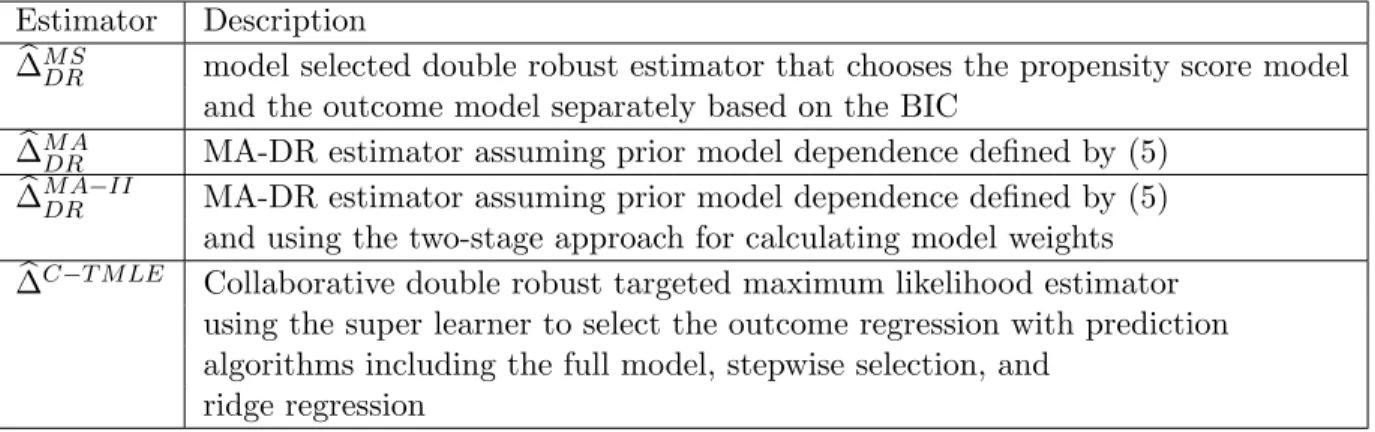
Table 1: Description of all estimators used in the simulations. Included is (1) the type of estimator; and (2) the choice of prior distribution for the model space. All Bayes factors are estimated using the BIC approximation.
Estimator Description
b
∆M SDR model selected double robust estimator that chooses the propensity score model and the outcome model separately based on the BIC
b
∆M ADR MA-DR estimator assuming prior model dependence defined by (5)
b
∆M ADR−II MA-DR estimator assuming prior model dependence defined by (5) and using the two-stage approach for calculating model weights
b
∆C−T M LE Collaborative double robust targeted maximum likelihood estimator using the super learner to select the outcome regression with prediction algorithms including the full model, stepwise selection, and
ridge regression
Table 2: Summary of Parameters for Simulation Group 1. In each of the 4 scenarios considered, we generate data as follows: (1) C1, ..., C5 iid∼ N(0,1); (2) X ∼ Bernoulli(p = expit(Cαps)); and (3) Y ∼
N(βX+Cαom, σ2) with β= 1 andσ2 = 4. All effects of confounders are linear on both the treatment and outcome.
Scenario Description αps (PS model) αom (Outcome model)
1 No confounding (0.4,0.3,0.2,0.1,0) (0,0,0,0,0) 2 Moderate confounding (0.5,0.5,0.1,0,0) (0.5,0,1,0.5,0) 3 Strong predictors of outcome, (0.1,0.1,1,1,1) (2,2,0,0,0)
weak predictors of treatment
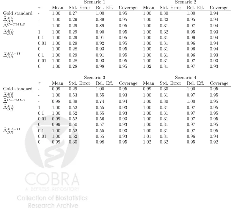
Table 3: The mean, standard error, relative efficiency (variance of the gold standard divided by the variance of the estimator), and 95% confidence interval coverage probability of various estimators when n = 200 and p= 5 for 1000 replications of the data.
Scenario 1 Scenario 2
τ Mean Std. Error Rel. Eff. Coverage Mean Std. Error Rel. Eff. Coverage Gold standard - 1.00 0.27 1.00 0.95 1.00 0.30 1.00 0.94 b ∆M S DR - 1.00 0.29 0.89 0.95 1.00 0.32 0.95 0.94 b ∆C−T M LE - 1.00 0.29 0.89 0.95 1.00 0.31 0.97 0.94 b ∆M A DR 1 1.00 0.29 0.90 0.95 1.00 0.32 0.95 0.93 0.1 1.00 0.29 0.91 0.95 1.00 0.31 0.96 0.94 0.01 1.00 0.29 0.92 0.95 1.00 0.31 0.96 0.94 0 1.00 0.28 0.93 0.95 1.00 0.31 0.96 0.94 b ∆M ADR−II 0.1 1.00 0.29 0.91 0.95 1.00 0.31 0.96 0.93 0.01 1.00 0.28 0.93 0.95 1.00 0.31 0.97 0.93 0 1.00 0.28 0.98 0.95 1.02 0.31 0.97 0.93 Scenario 3 Scenario 4
τ Mean Std. Error Rel. Eff. Coverage Mean Std. Error Rel. Eff. Coverage Gold standard - 0.99 0.29 1.00 0.95 0.99 0.30 1.00 0.95 b ∆M S DR - 1.00 0.53 0.55 0.93 1.00 0.31 0.97 0.95 b ∆C−T M LE - 0.98 0.39 0.74 0.94 1.00 0.30 1.00 0.95 b ∆M A DR 1 1.00 0.52 0.55 0.93 1.00 0.31 0.97 0.95 0.1 1.00 0.52 0.55 0.93 1.00 0.31 0.97 0.95 0.01 0.99 0.52 0.56 0.93 1.00 0.31 0.97 0.95 0 0.99 0.50 0.57 0.93 1.00 0.31 0.97 0.95 b ∆M ADR−II 0.1 1.00 0.52 0.55 0.93 1.00 0.31 0.97 0.95 0.01 1.00 0.52 0.55 0.93 1.01 0.31 0.96 0.94 0 0.99 0.30 0.98 0.95 1.02 0.32 0.95 0.92
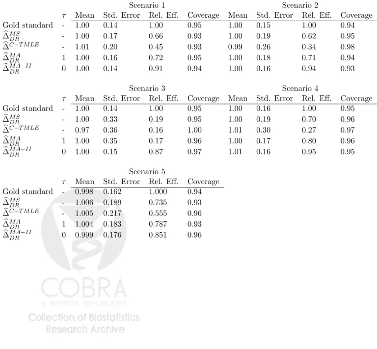
Table 4: The mean, standard error, relative efficiency (variance of the gold standard divided by the variance of the estimator), and 95% confidence interval coverage probability of various estimators when n = 200 and p= 100 for 500 replications of the data.
Scenario 1 Scenario 2
τ Mean Std. Error Rel. Eff. Coverage Mean Std. Error Rel. Eff. Coverage Gold standard - 1.00 0.14 1.00 0.95 1.00 0.15 1.00 0.94 b ∆M SDR - 1.00 0.17 0.66 0.93 1.00 0.19 0.62 0.95 b ∆C−T M LE - 1.01 0.20 0.45 0.93 0.99 0.26 0.34 0.98 b ∆M ADR 1 1.00 0.16 0.72 0.95 1.00 0.18 0.71 0.94 b ∆M ADR−II 0 1.00 0.14 0.91 0.94 1.00 0.16 0.94 0.93 Scenario 3 Scenario 4
τ Mean Std. Error Rel. Eff. Coverage Mean Std. Error Rel. Eff. Coverage Gold standard - 1.00 0.14 1.00 0.95 1.00 0.16 1.00 0.95 b ∆M SDR - 1.00 0.33 0.19 0.95 1.00 0.19 0.70 0.96 b ∆C−T M LE - 0.97 0.36 0.16 1.00 1.01 0.30 0.27 0.97 b ∆M ADR 1 1.00 0.35 0.17 0.96 1.00 0.17 0.80 0.96 b ∆M ADR−II 0 1.00 0.15 0.87 0.97 1.01 0.16 0.95 0.95 Scenario 5
τ Mean Std. Error Rel. Eff. Coverage Gold standard - 0.998 0.162 1.000 0.94 b ∆M SDR - 1.006 0.189 0.735 0.93 b ∆C−T M LE - 1.005 0.217 0.555 0.96 b ∆M ADR 1 1.004 0.183 0.787 0.93 b ∆M ADR−II 0 0.999 0.176 0.851 0.96
Table 5: Scenario 3: the mean posterior inclusion probabilities whenn= 200 andp= 5 for 1000 replications of the data.
Outcome Propensity score
τ C1 C2 C3 C4 C5 C1 C2 C3 C4 C5 b ∆M ADR 1 1 1 0.12 0.12 0.12 0.15 0.15 1 1 1 0.1 1 1 0.13 0.14 0.13 0.15 0.15 1 1 1 0.01 1 1 0.22 0.23 0.23 0.15 0.15 1 1 0.99 0 1 1 0.99 0.99 0.98 0.15 0.15 0.99 0.99 0.98 b ∆M ADR−II 1 1 1 0.12 0.12 0.12 0.15 0.15 1 1 1 0.1 1 1 0.12 0.12 0.12 0.15 0.15 1 1 1 0.01 1 1 0.12 0.12 0.12 0.15 0.15 1 1 1 0 1 1 0.12 0.12 0.12 0.14 0.14 0.12 0.12 0.12
Model specific doub
le rob
ust estimator
0.00
0.05
0.10
0.15
Figure 1: Model specific double robust estimator for the glioblastoma example and corresponding 95% confidence intervals for 1000 randomly chosen outcome models and 1000 randomly chosen propensity score models, sorted by point estimates. The unadjusted estimator (X), the model averaged double robust estimator (square), the double robust estimator that includes all covariates into both models (circle), and the model selected double robust estimator (triangle) are included. Model selection is performed using BIC.
Table 6: Baseline characteristics (% experiencing) and 1-year mortality rate for patients treated with temo-zolomide plus radiotherapy and radiotherapy alone, along with estimated inclusion probabilities (assuming prior model dependence defined by (5) and using the two-stage approach with τ = 0) for the analyses of the Medicare data.
Radiotherapy only Temozolomide (n= 1111) (n= 776) P r Inclusion in outcome model P r Inclusion in propensity score Age group: 65-69 25.6 30.7 Reference Reference 70-74 28.1 32.1 1.00 0.07 75-79 23.8 23.3 1.00 0.09 ≥80 22.5 13.9 1.00 0.95 Gender (female/male) 47.1 48.5 0.09 0.08 Married (yes/no) 64.9 71.0 0.03 0.03 Race (white/other) 85.4 89.9 0.10 0.10 Income (high/low) 63.0 67.8 1.00 0.23 Region:
Northeast 21.7 20.3 Reference Reference
Midwest 14.5 13.1 0.06 0.06
South 17.6 21.5 0.01 0.01
West 46.2 45.1 0.03 0.03
Dual eligible (yes/no) 14.3 11.6 0.02 0.02
Biopsy (yes/no) 31.1 28.9 0.02 0.02
Resection (yes/no) 73.2 79.1 1.00 0.48
CT scan(yes/no) 79.6 76.8 1.00 0.08
MRI (yes/no) 76.5 83.4 0.13 0.13
Initial discharge (home/other) 45.4 55.3 1.00 0.94
Number of tumors (1 tumor/>1 tumor) 97.5 98.2 0.02 0.02 Location of tumors (supratentorial/other) 77.6 78.5 0.04 0.04
Tumor size (≥3cm) 70.3 70.4 0.03 0.03
Palliative care (yes/no) 10.6 10.4 0.02 0.02
Extent of resection (major/minimal) 28.5 29.9 1.00 0.14
Atherosclerosis (yes/no) 17.8 14.4 0.72 0.05
Hypertension (yes/no) 61.5 61.5 0.02 0.02
Cerebrovascular disease (yes/no) 1.40 0.8 0.04 0.04
COPD (yes/no) 10.3 7.7 0.03 0.03
Pneumonia (yes/no) 1.0 1.3 0.01 0.01
Malnutrition (yes/no) 1.7 1.3 0.01 0.01
Dementia (yes/no) 7.6 5.9 0.02 0.02
Functional disability (yes/no) 0.3 0.0 0.02 0.02
Prior trauma (yes/no) 2.8 2.6 0.03 0.03
Psychological disease (yes/no) 2.3 2.1 0.01 0.01
Parkinson or Huntington (yes/no) 0.9 0.6 0.01 0.01
Anemia (yes/no) 8.2 9.1 0.02 0.01 Depression (yes/no) 5.0 5.2 0.06 0.05 Asthma (yes/no) 3.0 1.7 0.01 0.01 Diabetes (yes/no) 21.0 20.4 0.99 0.06 Deyo score: 0 57.9 61.1 Reference Reference 1 27.6 27.8 0.04 0.04 2+ 14.5 11.1 0.01 0.01