Laurent: Maastricht University, The Netherlands; Université Catholique de Louvain, CORE, B-1348, Louvain-la-Neuve, Belgium. Address : Department of Quantitative Economics, Maastricht University, School of Business and Economics, P.O. Box 616, 6200 MD, The Netherlands. Tel.: +31 43 3883843; Fax: +31 43 3884874
Rombouts: Institute of Applied Economics, HEC Montréal, CIRANO, CIRPÉE; Université Catholique de Louvain, CORE, B-1348, Louvain-la-Neuve, Belgium. Address : 3000 Côte Sainte-Catherine, Montréal (QC) Canada H3T 2A7. Tel.: +1 514 3406466; Fax: +1 514 3406469
Violante: Université de Namur, CeReFim; Université Catholique de Louvain, CORE, B-1348, Louvain-la-Neuve, Belgium. Address : FUNDP-Namur, Département des Sciences Économiques, Rempart de la Vierge, 8, B-5000, Namur. Tel. +32 81 724810; Fax: +32 81 724840
We would like to thank Luc Bauwens, Raouf Boucekkine, Lars Stentoft, Mohammed Bouaddi, Giovanni Motta, the participants to the 2nd International Workshop of the ERCIM Working Group on Computing and Statistics, the 64th European Meeting of the Econometric Society, the 26th annual meeting of the Canadian Econometric Study Group and the 9th Journées du CIRPÉE for their helpful comments. Financial support from the CREF-HEC Montreal and the Belgian Program on Interuniversity Poles of Attraction initiated by the Belgian State Prime Minister’s Office, science policy programming, is gratefully acknowledged. The usual disclaimer applies.
Cahier de recherche/Working Paper 09-48
On Loss Functions and Ranking Forecasting Performances of
Multivariate Volatility Models
(previously circulating asConsistent Ranking of Multivariate Volatility Models)
Sébastien Laurent Jeroen V.K. Rombouts Francesco Violante
Abstract:
A large number of parameterizations have been proposed to model conditional variance dynamics in a multivariate framework. However, little is known about the ranking of multivariate volatility models in terms of their forecasting ability. The ranking of multivariate volatility models is inherently problematic because it requires the use of a proxy for the unobservable volatility matrix and this substitution may severely affect the ranking. We address this issue by investigating the properties of the ranking with respect to alternative statistical loss functions used to evaluate model performances. We provide conditions on the functional form of the loss function that ensure the proxy-based ranking to be consistent for the true one – i.e., the ranking that would be obtained if the true variance matrix was observable. We identify a large set of loss functions that yield a consistent ranking. In a simulation study, we sample data from a continuous time multivariate diffusion process and compare the ordering delivered by both consistent and inconsistent loss functions. We further discuss the sensitivity of the ranking to the quality of the proxy and the degree of similarity between models. An application to three foreign exchange rates, where we compare the forecasting performance of 16 multivariate GARCH specifications, is provided.
Keywords: Volatility, Multivariate GARCH, Matrix norm, Loss function, Model
confidence set
1
Introduction
A special feature of economic forecasting compared to general economic modeling is that we can measure a model’s performance by comparing its forecasts to the outcomes when they become available. Generally, several forecasting models are available for the same variable and forecasting performances are evaluated by means of a loss function. Elliott and Timmermann (2008) provide an excellent survey on the state of the art of forecasting in economics. Details on volatility and correlation forecasting can be found in Andersen, Bollerslev, Christoffersen, and Diebold (2006).
The evaluation of the forecasting performance of volatility models raises the problem that the variable of interest (i.e., volatility) is unobservable and therefore the evaluation of the loss function has to rely on a proxy. However this substitution may induce a distortion with respect to the true ordering (based on the unobservable volatility). The impact on the ordering of the substitution of the true volatility by a proxy has been investigated for univariate models by Hansen and Lunde (2006a). They provide conditions, for both the loss function and the volatility proxy, under which the approximated ranking (based on the proxy) is consistent for the true ranking. Starting from this result, Patton (2009) derives necessary and sufficient conditions on the functional form of the loss function for the latter to order consistently. These results have important implications on testing procedures for superior predictive ability (see Diebold and Mariano (1995), West (1996), Clark and McCracken (2001), the reality check by White (2000) and the recent contributions of Hansen and Lunde (2005) with the superior predictive ability (SPA) test and Hansen, Lunde, and Nason (2009) with the Model Confidence Set test, among others), because when the target variable is unobservable, an unfortunate choice of the loss function may deliver unintended results even when the testing procedure is formally valid. In fact, with respect to ranking multivariate volatility model forecast performances, where conditional variance matrices are compared, little is known about the properties of the loss function. This is the first paper that addresses this issue.
In this paper, we unify and extend the results in the univariate framework to the evaluation of multivariate volatility models, that is the comparison and ordering of sequences of variance matrices. From a methodological viewpoint, we first extend to the multivariate dimension
from the CREF-HEC Montreal and the Belgian Program on Interuniversity Poles of Attraction initiated by the Belgian State Prime Minister’s Office, science policy programming, is gratefully acknowledged. The usual disclaimer applies.
the conditions that a loss function has to satisfy to deliver the same ordering whether the evaluation is based on the true conditional variance matrix or an unbiased proxy of it. Second, similar to the univariate results in Patton (2009), we state necessary and sufficient conditions on the functional form of the loss function to order consistently in matrix and vector spaces. Third, we identify a large set of parameterizations that yield loss functions able to preserve the true ranking. Although we focus on homogeneous loss functions, unlike in the univariate case, a complete identification of the set of consistent loss functions is not available. This is because in the multivariate case there is an infinite number of possible combinations of the elements of the forecasting error matrix which yield a loss function that satisfies the necessary and sufficient conditions. We identify a number of well known vector and matrix loss functions, many of which are frequently used in practice, categorized with respect to different characteristics such as the degree of homogeneity, shape, etc. Furthermore, given the necessary and sufficient functional form, other loss functions, well suited for specific applications, can easily be derived.
Note that different loss functions may deliver different rankings depending on the charac-teristics of the data that each loss function is able to capture. We find that many commonly used loss functions do not satisfy the conditions for consistent ranking. However, these loss functions show desirable properties (e.g., down weighting extreme forecast errors) which can be useful in applications. We show that inconsistent loss functions are not per se inferior, and, under certain conditions they can still deliver a ranking that is insensitive under the use of a proxy. With respect to terminology, consistency of the ranking does not mean invariance of the ordering. Consistency is in fact intended only with respect to the accuracy of the proxy and for a given loss function, i.e., consistency between the true and the approximated ranking. On the other hand, invariance of the ranking means that the ordering does not change with respect to the choice of the loss function.
To make our theoretical results concrete, we focus on multivariate GARCH models to forecast the conditional variance matrix of a portfolio of financial assets. Through a com-prehensive Monte Carlo simulation, we study the impact of the deterioration of the quality of the proxy on the ranking of multivariate GARCH models with respect to different choices for the loss function. The true model is a multivariate diffusion from which we compute the integrated covariance, i.e., the true daily variance matrix. The multivariate GARCH models
are estimated on daily returns and used to compute 1-step ahead forecasts. The proxy of the daily variance matrix is realized covariance as defined in Andersen, Bollerslev, Diebold, and Labys (2003). The quality of this proxy is controlled through the level of aggregation of the simulated intraday data used to compute Realized Covariance. The main conclusion of our simulation is that, when ranking over a discrete set of volatility forecasts, inconsistent loss functions are not per se inferior to consistent ones. When the quality of the proxy is sufficiently good, consistency between the true and the approximated ranking can still be achieved. The break even point, in terms of level of accuracy of the proxy, after which the bias starts to affect the ranking, depends on the trade-off quality of the proxy vs. degree of similarity between models. That is, the closer the forecast error matrices, the higher the accuracy of the proxy needed to correctly discriminate between competing models.
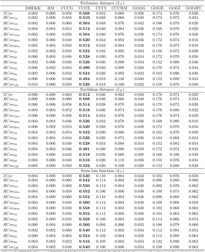
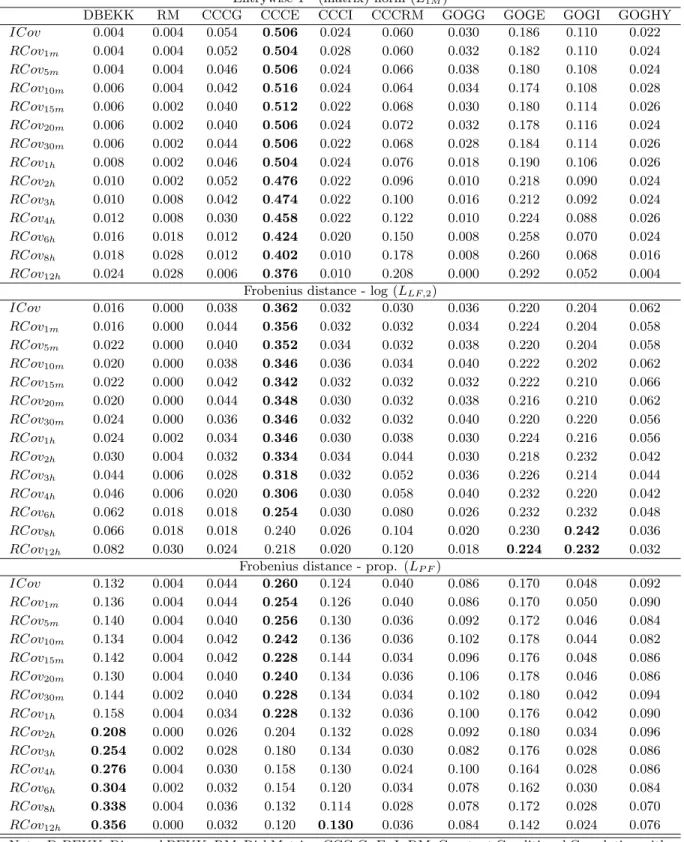
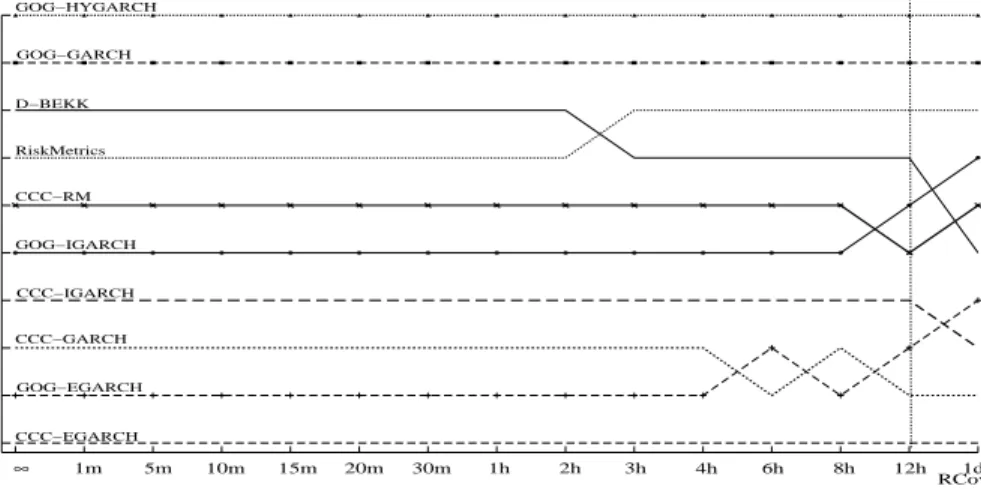
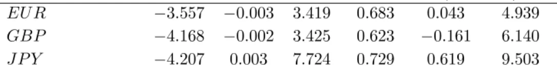
We illustrate our findings using three exchange rates (Euro, UK pound and Japanese yen against US dollar). We consider 16 multivariate GARCH specifications which are frequently used in practice. The advantage of choosing a consistent loss function to evaluate model performances is striking. The ranking based on an inconsistent loss function, together with an uninformative proxy, is found to be severely biased. In fact, as the quality of the proxy deteriorates inferior models emerge and outperform models which are otherwise preferred when the comparison is based on a more accurate proxy.
The rest of the paper is organized as follows. Section 2 develops conditions for consistent ranking and derives the admissible functional form of the loss function. We discuss how to build a class of consistent loss functions and give remarks on inconsistent loss functions. Sec-tion 3 provides first a brief overview of the multivariate GARCH specificaSec-tions considered in this paper and second, it introduces the realized covariance, used as a proxy for the unob-served conditional variance matrix. A detailed simulation study in Section 4 investigates the robustness of the ranking subject to consistent and inconsistent loss functions with respect to the level of accuracy of the proxy. The empirical application to three exchange rates is presented in Section 5. Section 6 concludes and discusses directions for further research. All proofs are provided in Appendix A. Supporting examples are given in Appendix B.
2
Consistent ranking and distance metrics
As explained in Andersen, Bollerslev, Christoffersen, and Diebold (2006), the problem when comparing and ranking forecasting performance of volatility models is that the true condi-tional variance is unobservable so that a proxy for it is required. Let us define the true, or underlying, ordering between volatility models as the ranking implied by a loss function, eval-uated with respect to the unobservable conditional variance. The substitution of the latter by a proxy may introduce, because of its randomness, a ranking of volatility models that differs from the true one. Hansen and Lunde (2006a) provide a theoretical framework for the analysis of the ordering of stochastic sequences and identify conditions that a loss function has to satisfy to deliver an ordering consistent with the true ranking when a proxy for the conditional variance is used. Patton (2009) derives necessary and sufficient conditions on the functional form of the loss function for the latter to order consistently. In particular, he finds that the necessary and sufficient functional form relates to the linear exponential family of objective functions (see Gourieroux and Monfort (1995) for details).
In this section, we extend and unify these results to the case of multivariate volatility models, which requires the comparison and ordering of sequences of variance matrices. In the following subsections, we first set the notation, working assumptions and basic definitions and, as an example, we introduce a set of loss functions commonly used in a multivariate volatility context. Second, we discuss the conditions for a loss function to give a consistent ranking. Third, we characterize the functional form of a consistent loss function. Fourth, we illustrate how consistent loss functions can be constructed in practice.
2.1 Notation and definitions
We first fix the notation and make explicit what we mean by a well defined loss function and by consistent ranking. For N time series at time t we denote RN++×N the space of N ×N positive definite matrices and ˙H ⊂ RN++×N a compact subset of R++N×N. H˙ represents the set of candidate models with typical element indexed by m,Hm,t such that Hm,t ∈ H˙. R+ denotes the positive part of the real line. We define L(·,·) an integrable loss function L : RN++×N×H˙ →R+such thatL(Σt, Hm,t) is the loss evaluated using the true but unobservable conditional variance matrix Σtwith respect to modelm. We refer to the ordering based on the expected loss, E[L(Σt, Hm,t)] as the true ordering. Similarly,L( ˆΣt, Hm,t) is the loss evaluated
using ˆΣt, a proxy of Σt, and E[L( ˆΣt, Hm,t)] determines the approximated ranking. When needed, we also refer to the empirical ranking as the one based on the sample evaluation of L( ˆΣt, Hm,t), i.e.,T−1
t
L( ˆΣt, Ht), whereT is the length of the forecast sample. The set,t−1 denotes the information at timet−1 and Et−1(·) ≡E(·|t−1) the conditional expectation. The elements, σi,j,t, ˆσi,j,t and hi,j,t indexed by i, j = 1, ..., N, refer to the elements of the matrices Σt, ˆΣt, Ht respectively. Furthermore, σk,t, ˆσk,t and hk,t are the elements, indexed by k = 1, ..., N(N + 1)/2, of the vectors σt = vech(Σt), ˆσt = vech( ˆΣt) and ht = vech(Ht) respectively, wherevech(·) is the operator that stacks the lower triangular portion of a matrix into a vector. Finally, the vectorized difference between the true variance matrix and its proxy is denoted byξt= (ˆσt−σt).
The following assumptions ensure that the loss functionL(·,·) is able to correctly order with respect to the true variance matrix.
A1.1 L(·,·) is continuous in ˙H and it is uniquely minimized at Ht∗ which represents the optimal forecast. If Ht∗∈int( ˙H), L(·,·) is convex in ˙H.
A1.2 L(·,·) is such that the optimal forecast equals the true conditional variance Σt, Ht∗ = arg min
Ht∈H˙
L(Σt, Ht)⇔Ht∗= Σt. (1)
A1.3 L(Σt, Ht) = 0 ⇔ Ht= Σt, i.e., the loss function yields zero loss whenHt∗ = Σt.
Definition 1 Under assumptions A1.1 to A1.3, the loss function is well defined.
The notion of consistency of ranking is defined as follows:
Definition 2 Consistency between the true ranking and the ordering based on a proxy is achieved if
E(L(Σt, Hl,t))≥E(L(Σt, Hm,t))⇔E(L( ˆΣt, Hl,t))≥E(L( ˆΣt, Hm,t)) (2)
is true for all l=m, where L(·,·) is a well defined loss function in the sense of Definition 1 and Σˆt is some conditionally unbiased proxy of Σt.
By Definition 2, the ranking between any two models indexed by l and m, is consistent if it is the same whether it is based on the true conditional variance matrix or a conditionally unbiased proxy. Note that conditional unbiasedness is sufficient to ensure consistency as defined in Definition 2.
As underlined in Patton (2009) it is common practice to use several alternative measures of forecast accuracy to respond to the concern that some particular characteristics of the data may affect the result. As an example, we discuss next a selection of loss functions, listed in Table 1, which are commonly used to evaluate multivariate model performances based on forecast accuracy, or, in a more general context, to measure the distance between matrices and vectors (see Ledoit and Wolf (2003), James and Stein (1961), Bauwens, Lubrano, and Richard (1999), Koch (2007), Herdin, Czink, Ozcelik, and Bonek (2005)) and provide their classification. Although the loss function listed below are in principle well suited to measure variance forecast performances, it turns out that several are inappropriate in this setting.
Table 1: Loss functions and their classification
Matrix loss functions
LF Frobenius distance 1≤i,j≤N(σi,j,t−hi,j,t)2 consistent LS Stein distance T r[Ht−1Σt]−logHt−1Σt−N consistent L1M Entrywise 1 - (matrix) norm 1≤i,j≤N|σi,j,t−hi,j,t| inconsistent LP F Proportional Frobenius dist. T r(ΣtHt−1−I)2 inconsistent LLF,1 Log Frobenius distance (1) logΣtHt−12 inconsistent LLF,2 Log Frobenius distance (2)
log T r[ΣtΣt]
T r[HtHt] 2
inconsistent LCor Correlation distance 1−√ T r(ΣtHt)
T r(ΣtΣt)T r(HtHt) ∈
[0,1] inconsistent Vector loss functions
LE Euclidean distance 1≤k≤N(N+1)/2(σk,t−hk,t)2 consistent LW E Weighted Euclidean distance (σt−ht)W(σt−ht) consistent
(with matrix of weightsW)
L1V Entrywise 1 - (vector) norm 1≤k≤N(N+1)/2|σk,t−hk,t| inconsistent
The first loss function,LF, is the natural extension to matrix spaces of the mean squared error (MSE). The second, LS, is the scale invariant loss function introduced by James and Stein (1961). L1M represents the extension to matrix spaces of the mean absolute deviation (MAD) and is known as the entrywise 1 - (matrix) norm. LP F is the extension of the
heteroskedasticity adjusted MSE and is a quadratic loss function with the same parametric form of the Frobenius distance but which measures deviations in relative terms (see James and Stein (1961)). We refer to this loss function as proportional Frobenius distance. LLF,1 and LLF,2 are adaptations of the MSE logarithmic scale. In particular, the loss function in LLF,2, alternatively defined as
logiλ2(Σt)i iλ2(Ht)i−1 2, considers the singular values as a summary measure of a matrix. The sum of squared singular values (defined as
iλ2(A)i = T r(AA)) represents the Frobenius distance of Σt and Ht from 0. The ratio
measures the discrepancy in relative terms while the logarithm ensures that deviations are measured as factors and the squaring ensures that factors are equally weighted. We refer to this loss function as log Frobenius distance. LCor is also based on the Frobenius distance but it exploits the Cauchy-Shwartz inequality. In fact, by the inequality, the ratio is equal to one when Ht= Σt and tends to 0 if Ht and Σtdiffer to a maximum extent. The ratio resembles to a correlation coefficient between the matrices Ht and Σt. LE is the Euclidean distance computed on all unique elements of the forecast error matrix, whileLW E is a weighted version of LE. The last function, L1V, also represents an extension of the mean absolute deviation (MAD) but the distance is defined on a vector space. It differs fromL1M for equally weighting the unique elements of the forecast error matrix.
2.2 Conditions for consistent ranking of multivariate volatility models
We provide sufficient conditions that a loss function has to satisfy to deliver the same ordering whether the evaluation is based on the true conditional variance matrix or a proxy. To make the exposition easier, we can redefine without loss of generality the functionL(·,·) from the space R++N×N×H˙ toR+ as a function fromRN(N+1)/2×H →˙ R+, withvech(Hm,t)∈H˙ and
˙
H ⊂ RN(N+1)/2, of all unique elements of the matrices Σt and Ht since these are variance matrices and therefore symmetric. This simplification allows to ignoreN(N−1)/2 redundant first order conditions in the minimization problem defined in (1). We make use of the following assumptions:
A2.1 L(Σt, Ht) and L( ˆΣt, Ht) have the same parametric form ∀Ht ∈ H˙ so that uncertainty depends only on ˆΣt.
A2.3 L(·,·) is twice continuously differentiable with respect to ˆσt and ht.
A2.4 ξt= (ˆσt−σt) is a vector martingale difference sequence with respect to t with finite conditional variance matrix Vt=Et−1[ξtξt].
Proposition 1 states a sufficient condition on the loss function to ensure consistent ranking.
Proposition 1 Under assumptions A2.1 to A2.4, a well defined loss function in the sense of Definition 1 with ∂2L(Σt,Ht)
∂σl,t∂σm,t finite and independent of Ht ∀l, m = 1, ..., N(N + 1)/2 is
consistent in the sense of Definition 2.
The proof is given in Appendix A. Proposition 1 applies for any conditionally unbiased proxy independently of its level of accuracy. The difference between the true and the approximated ordering which is likely to occur whenever Proposition 1 is violated, is denoted as the ob-jective bias. The bias must not be confused with sampling variability, that is the distortion between the approximated and the empirical ranking. In fact, while the latter tend to dis-appear asymptotically (i.e., T−1
t
L( ˆΣt, Ht) →p E
L( ˆΣt, Ht) under ergodic stationarity of E
L( ˆΣt, Ht) ), the presence of the objective bias may induce the sample evaluation to be inconsistent for the true one irrespectively of the sample size. Note that, from the set of loss functions given in Table 1, it is straightforward to show that only LF,LS,LE andLW E satisfy Proposition 1.
We can further discuss the implications of Proposition 1 and elaborate on the case when Proposition 1 is violated. We show that the bias between the true and the approximated ranking depends on the accuracy of the proxy for the variance matrix: the presence of noise in the volatility proxy introduces a distortion in the approximated ordering, which tends to disappears when the accuracy of the proxy increases. More formally, consider a sequence of volatility proxies ˆΣ(ts) indexed bysand denote Ht∗(s) such that
Ht∗(s)= arg min
Ht∈intH˙
Et−1[L( ˆΣt(s), Ht)]. (3)
Furthermore, we need the following additional assumption for the next proposition:
A2.5 The volatility proxy satisfiesEt−1[ξt(s)] = 0∀sandVt(s) =Et−1[ξt(s)ξt(s)]→p 0 ass→ ∞.
Proposition 2 Under assumptions A2.1 to A2.5, for a well defined loss function in the sense of Definition 1, it holds:
i) If ∂3L(Σt,Ht)
∂σt∂σt∂hk,t = 0 ∀k, then H
∗(s)
t = Σt ∀s,
ii) If ∂3L(Σt,Ht)
∂σt∂σt∂hk,t = 0 for some k, then H
∗(s) t
p
→Σt as s→ ∞.
The proof is given in Appendix A. The first statement states that, under Proposition 1, the optimal forecast is the conditional variance, and consistency is achieved regardless of the quality of the proxy. The second result in Proposition 2 shows that the distortion introduced in the ordering when using an inconsistent loss function tends to disappear as the quality of the proxy improves. Therefore, when ordering over a discrete set of models, a loss function that violates Proposition 1 may still deliver a ranking consistent to the one implied by the true conditional variance matrix, if a sufficiently accurate proxy is used in the evaluation. In other words, when the variance of the proxy is small with respect to discrepancy between any two models, the distortion induced by the proxy becomes negligible, leaving the ordering unaffected. In the simulation study in Section 4, we further investigate this issue and in particular investigate the relationship between the accuracy of the proxy (i.e., the variability of the proxy) and the degree of similarity between model performances (i.e., how close performances are). However, in practice, it may be difficult to determine ex-ante the degree of accuracy of a proxy. Since the trade off accuracy vs. similarity is difficult to quantify ex-ante, model comparison and selection based on inconsistent loss function becomes unreliable and may lead to undesired results. The empirical application in Section 5 reveals that a sufficiently accurate proxy may not be available.
2.3 Functional form of the consistent loss function
In the univariate framework, Patton (2009) identifies necessary and sufficient conditions on the functional form of the loss function to ensure consistency between the true ranking and the one based on a proxy for the variance. The set of consistent loss functions relate to the class of linear exponential densities of Gourieroux, Monfort, and Trognon (1984) and partially coincides with the subset of homogeneous loss functions associated with the most important linear exponential densities. In fact, the family of loss functions with degree of homogeneity equal to zero, one and two defined in Patton (2009), can be alternatively derived from the objective functions corresponding to the Gaussian, Poisson and Gamma densities respectively (see Gourieroux and Monfort (1995) for more details).
We propose necessary and sufficient conditions on the functional form of the loss function defined such that it is well suited to measure distances in matrix and vector spaces. Although, unlike in the univariate case, a complete identification of the set of consistent loss functions is not feasible, we are able to identify a large set of parameterizations which yield consistent loss functions. We show that several well known vector and matrix distance functions also belong to this set.
In order to proceed, we need the following assumptions:
A3.1 Σˆt|t−1 ∼Ft∈F the set of absolutely continuous distribution functions of R++N×N;
A3.2 ∃Ht∗ ∈int( ˙H) such thatHt∗ =Et−1( ˆΣt);
A3.3 Et−1 L( ˆΣt, Ht) <∞ for someH ∈H˙,Et−1 ∂L(ˆΣt,Ht) ∂ht Ht=Σt <∞and Et−1 ∂L(ˆΣt,Ht) ∂ht∂ht Ht=Σt
<∞for alltwhere the last two inequalities hold elementwise. Note that A3.2 follows directly from A1.2 and A2.4 because Ht∗ ∈int( ˙H) implies Ht∗ = Σt by A1.2 while Et−1( ˆΣt) = Σt results from A2.4. Assumption A3.4 allows to interchange differentiation and expectation, see L’Ecuyer (1990) and L’Ecuyer (1995) for details.
Proposition 3 Under assumptions A2.3, A2.4 and A3.1 to A3.3 a well defined loss function, in the sense of Definition 1, is consistent in the sense of Definition 2 if and only if it takes the form
L( ˆΣt, Ht) = ˜C(Ht)−C˜( ˆΣt) +C(Ht)vech( ˆΣt−Ht), (4)
where C˜(·) is a scalar valued function from the space of N ×N positive definite matrices to
R, three times continuously differentiable with
C(Ht) = ∇C˜(Ht) = ⎡ ⎢ ⎢ ⎣ ∂C˜(Ht) ∂h1,t .. . ∂C˜(Ht) ∂hK,t ⎤ ⎥ ⎥ ⎦ C(Ht) = ∇2C˜(Ht) = ⎡ ⎢ ⎢ ⎣ ∂C˜(Ht) ∂h1,t∂h1,t · · · ∂C˜(Ht) ∂h1,t∂hK,t .. . . .. ∂C˜(Ht) ∂hK,t∂h1,t ∂C˜(Ht) ∂hK,t∂hK,t ⎤ ⎥ ⎥ ⎦
the gradient and the hessian of C˜(·) with respect to the K=N(N + 1)/2 unique elements of
Ht and C(Ht) negative definite.
Corollary 1 GivenΣˆtandHtsymmetric and positive definite, then the loss function specified in (4) is isometric to
L( ˆΣt, Ht) = ˜C(Ht)−C˜( ˆΣt) +T r[ ¯C(Ht)( ˆΣt−Ht)], (5)
with C˜(·) defined as in Proposition 3 and
¯ C(Ht) = ⎡ ⎢ ⎢ ⎢ ⎢ ⎢ ⎣ ∂C˜(H) ∂h1,1,t 1 2∂ ˜ C(H) ∂h1,2,t ... 1 2 ∂ ˜ C(H) ∂h1,N,t 1 2∂ ˜ C(H) ∂h1,2,t ∂C˜(H) ∂h2,2,t .. . . .. 1 2∂ ˜ C(H) ∂h1,N,t ∂C˜(H) ∂hN,N,t ⎤ ⎥ ⎥ ⎥ ⎥ ⎥ ⎦ ,
where the derivatives are taken with respect to all N2 elements of Ht.
The proof is provided in Appendix A. Unlike in the univariate framework, the multivariate dimension offers a large flexibility in the formulation of the loss function, see Table 1 for several parameterizations. In applied work, a careful analysis of the functional form of the loss function is a crucial preliminary step to the selection based on the specific properties of a given loss function. In this respect, it is clear that Assumption A1.2 has a central role in this setting. It is interesting to elaborate on the case when A1.2 is dropped while keeping all other assumptions in place. We can show that, relaxing Proposition 1 and 2 and Definition 2 to admit loss functions badly formulated, still yields an ordering that is insensitive to the accuracy of the proxy, i.e. apparently consistent. However, when A1.2 is violated, such ordering is inherently invalid because the optimal forecast does not equal the true conditional variance. To illustrate this, starting from the functional form defined in Proposition 3, we consider the following generalization of (5)
L(Σt, Ht) = ˜C(Ht)−C˜(Σt) +f[ ¯C(Ht)(Σt−Ht)], (6) assuming that there exists a linear map f[·] : RN×N → R such that L(Σt, Ht) satisfies second order conditions. We summarize the implications of relaxing assumption A1.2 from Proposition 1, 2 and 3 in the following remark. The proof is given in Appendix A.
Remark 1 Define the true ordering between variance matrix forecasts, i.e., based on the true conditional variance matrix, and a the approximated ordering, i.e., based on the volatil-ity proxy. Under the loss function (6), if
i) f[·]≡ T r[·] (A1.2 is satisfied): and a are equivalent, in the sense of Definition 2, and L(Σt, Ht) is such that Ht∗=E( ˆΣt|t−1) = Σt, i.e., the loss function is well defined in the sense of Definition 1;
ii) f[·] ≡T r[·](A1.2 is violated): andaare equivalent, in the sense that the substitution of the true covariance by a proxy does not affect the ordering. However, L(Σt, Ht) is such that Ht∗ = E( ˆΣt|t−1) = Σt, i.e., the loss function points to an optimal forecast different from the true conditional variance independently from the use of a proxy.
The first part of Remark 1 reaffirms sufficiency and necessity of the functional form defined in Proposition 3. With respect to the second part, note that, under (6), the general idea of consistency of the ranking, i.e., equivalence of true and approximated ranking, is still valid. In fact, if f[·] is a linear map, then f[ ¯C(Ht)(Σt−Ht)] is linear in σi,j,t ∀i, j = 1, ..., N, and therefore, similarly to what stated in Proposition 1, it holds that∂2L(Σt, Ht)/∂σt∂σt∂hk,t = 0
∀k= 1, ..., N(N + 1)/2. This result ensures the ranking based on the volatility proxy to be apparently consistent for the one based on the true conditional variance and insensitive to the level of accuracy of the proxy. The objective bias does not represent an issue here: in absence of assumption A1.2, the underlying ordering will differ from any valid or acceptable ordering also when based on the true conditional variance. A badly defined loss function points to an optimal forecast different from the true conditional variance.
2.4 Building a class of consistent loss functions
Endowed with the functional form defined in Proposition 2 and Corollary 1, we illustrate how to recover several consistent loss functions. These loss functions can be categorized with respect to different characteristics, for instance the degree of homogeneity, the shape, the underlying family of distributions or the functional form for ˜C(·).
We start by investigating the case of loss functions that are based only on the forecast error, that is L( ˆΣt, Ht) =L( ˆΣt−Ht). Patton (2009) shows that in the univariate case the MSE loss function is the only consistent loss function that depends solely on the forecast error. The multivariate setting offers more flexibility in the functional form for a consistent loss function based on the forecast error. The following proposition defines the family of such loss functions.
Proposition 4 A loss function based only on the forecast error Σˆt−Htthat is consistent in the sense of Definition 2 is defined by the quadratic form
L( ˆΣt, Ht) =L( ˆΣt−Ht) =vech( ˆΣt−Ht)Λˆvech( ˆΣt−Ht) (7)
b) ∇2C˜(Ht) =−2 ˆΛ = Λ is a matrix of constants defined according to Proposition 3, c) Λˆ defines the weights assigned to the elements of the forecast error matrix Σˆt−Ht, d) symmetric under 180◦ rotation around the origin, i.e. L( ˆΣt−Ht) =L(Ht−Σˆt).
The proof is given in Appendix A. Proposition 4 defines a family of quadratic loss functions which depends on the choice of the matrix of weights ˆΛ. Formally, the quadratic polynomial in (7) defines a family of quadric surfaces, i.e., elliptic paraboloids, and ˆΛ defines the shape of the surface. As described above, the loss function in (7) corresponds to the MSE in the univariate case. In that case the loss function is symmetric, i.e., equally penalizes positive and negative forecast errors. The advantage of the multivariate case is that the notion of symmetry can be analyzed from a different aspect. Although L(., .) is symmetric under 180◦ rotation around the origin, a particular choice of ˆΛ can still generate some types of asymmetries. In the following, we derive and discuss the properties of some well known loss functions belonging to the family defined by Proposition 4.
The simplest parameterization of ˆΛ yield a loss function based on thevech() transforma-tion of the forecast error matrix, i.e., a loss functransforma-tion based on the notransforma-tion of distance on a vector space rather than a matrix space. Three examples are provided (in increasing order of generality). In Appendix B, we provide a series of analytical examples.
Example 1: Euclidean distance
From (7), by setting ˆΛ =IK we obtain a loss function of the form LE = (ˆσt−ht)IK(ˆσt−ht) =
1≤k≤K
(ˆσk,t−hk,t)2. (8)
The loss function defined in (8) is the square of the Euclidean norm on the vech() trans-formation of the forecast error matrix ( ˆΣt −Ht). The matrix ˆΛ is such that variances and covariances forecast errors are equally weighted. The loss function has mirror sym-metry about all coordinate planes, i.e., L((ˆσ1,t −h1,t), ...,(ˆσk,t −hk,t), ...,(ˆσK,t −hK,t)) = L((ˆσ1,t−h1,t), ...,−(ˆσk,t−hk,t), ....,(ˆσK,t −hK,t)) for all k, and is also symmetric under any rotation about the origin, e.g. L((ˆσt−ht)) =L(−(ˆσt−ht)). Equal weights also imply that LE is a symmetric polynomial, i.e., it is invariant under any permutation of the elements of (ˆσt−ht), that is, L((ˆσs1,t−hs1,t), ...,(ˆσsK,t−hsK,t)) = L((ˆσ1,t−h1,t), ...,(ˆσK,t−hK,t)) for some permutation s of the subscripts 1, ..., K. The contours of the Euclidean distance are, indeed, represented by spheres centered at the origin.
Example 2: Weighted Euclidean distance
A more flexible version of (8) is the weighted Euclidean distance, where ˆΛ is defined as ˆλi,i >0 and ˆλi,j = 0,i, j= 1, ..., K, that is
LW E = (ˆσt−ht)Λ(ˆˆ σt−ht) =
1≤k≤K
ˆ
λk,k(ˆσk,t−hk,t)2. (9)
This loss function allows to differently weight each variance and covariance forecast error. Also LW E shows mirror symmetry about all coordinate planes and it is also symmetric under a 180◦ rotation about the origin. However, unlike LE, it is not invariant to permutations of the elements of (ˆσt−ht), unless ˆλi,i = c for all i, i.e. LW E = cLE, where c is a constant. The first type of symmetry implies that for each element of the forecast error matrix over and under predictions are equally penalized. To illustrate the second type of symmetry we provide an example: For a given absolute forecast error |σˆt−ht|, i.e., fixing ˆσt and ht, consider LW E evaluated at the following points in the domain: i) LiW E, the loss at (ˆσk,t− hk,t) > 0 ∀k (all variances and covariances are under predicted) and ii) LiiW E, the loss at (ˆσt −ht) < 0 ∀k (all variances and covariances are over predicted). Then it holds that LiW E = LiiW E. Furthermore, consider LiiiW E, the loss at (ˆσk,t −hk,t) > (<)0, for some k (some variances/covariances are under predicted, while other are over predicted), then mirror symmetry implies LiW E =LiiW E =LiiiW E. Finally, the lack of invariance under permutations, i.e., LW E is not symmetric about the bisector planes, is induced by the unequal distribution of the weights to the elements of the forecasting errors matrix. The contours of the weighted Euclidean distance are represented by ellipsoids centered at the origin and with the axes of symmetry lying on the coordinate axes.
Example 3: Pseudo Mahalanobis distance
This loss function represents a generalization of (9). It is obtained by setting ˆλi,j > 0, i, j = 1, ..., K, that is
LM = (ˆσt−ht)Λ(ˆˆ σt−ht) =
1≤k,l≤K
ˆ
λk,l(ˆσk,t−hk,t)(ˆσl,t−hl,t). (10)
with ˆΛ chosen according to Proposition 4. We call the loss functions defined in (10) pseudo Mahalanobis distance because though it has the same parametric form, unlike the Maha-lanobis distance, the matrix of weights ˆΛ is deterministic and does not depend on (ˆσt−ht).
In this case, since ˆΛ is non diagonal,LM also includes the cross product of variances and covariances forecast errors. This loss function is only symmetric under a 180◦ rotation about the origin. The matrix ˆΛ here plays a role similar to a correlation in a multivariate symmetric distribution: positive (negative) weights imply that systematic over/under predictions are penalized less (more). To illustrate this type of symmetry, as before, consider, for a given absolute forecast error |σˆt−ht|,LM evaluated at the following points in the domain: i)LiM, the loss at (ˆσk,t−hk,t) >0 ∀k (all variances and covariances are under predicted), ii) Lii
M,
the loss at (ˆσt−ht)<0 ∀k (all variances and covariances are over predicted) and iii) LiiiW E, the loss at (ˆσk,t−hk,t)>(<)0, for some k(some variances/covariances are under predicted, while other are over predicted). Then it holds thatLiW E =LiiW E. However, sinceλi,j >(<)0, i=j, then LiW E = LiiW E =LiiiW E. Furthermore, LM is not invariant to permutations of the elements of (ˆσt−ht), unless ˆΛ is chosen such that LM = cLE, where c is a constant. The contours of the pseudo Mahalanobis distance are represented by ellipsoids centered at the origin and with the axes of symmetry, whose direction is given by the sign of the off diagonal elements of ˆΛ, that are rotated with respect to the coordinate axes.
The parameterization given in Proposition 4 allows to focus on the ordering implied by a subset of elements of the forecast error matrix. As an example, consider the comparison based on correlation matrices. In this case, one may want to focus on the elements of the strictly lower diagonal portion of the forecast error matrix, i.e., the N(N −1)/2 correlation forecast errors.
Remark 2 (Subsets of forecast errors) The loss function in (7) can be reparameterized using Λˆ diagonal and diag( ˆΛ) =vech(V) where V is symmetric with typical element, indexed byi, j= 1, ..., N(N+ 1)/2, vi,j = 0 ifi=j, vi,j = 0if i=j. Although in this caseΛˆ does not satisfy Proposition 4, the resulting loss function represents the weighted Euclidean distance on the vector holding the strictly lower diagonal elements of the forecast error matrix with weights vi,j, that is
LW E = (ˆσt−ht)Λ(ˆˆ σt−ht) =
1≤i<j≤N
vi,j(ˆσi,j,t−hi,j,t)2. (11)
In fact, define lvech() as the operator that stacks the strictly lower triangular portion of a matrix into a vector, σˆtlw = lvech( ˆΣt), hlwt = lvech(Ht) and diag( ˆΛlw) = lvech(V), (11) is equivalent to
LlwW E =lvech( ˆΣt−Ht) ˆΛlwlvech( ˆΣt−Ht) =
1≤k≤N(N−1)/2
ˆ
λlwk,k(ˆσk,tlw −hlwk,t)2,
We discuss next a particular parameterization of ˆΛ which leading to a loss function known as Frobenius distance. This loss function is based on the notion of distance on a matrix space rather then a vector space. It considers the entire forecast error matrix, therefore allowing to exploit some interesting matrix properties.
Example 4: Frobenius distance
From (7), if we set ˆΛ diagonal and diag( ˆΛ) = vech(V) where V is symmetric with typical element, indexed by i, j = 1, ..., N(N + 1)/2, vij = 1 if i = j, vij = 2 if i = j, then the resulting loss function is
LF =T r[( ˆΣt−Ht)( ˆΣt−Ht)]. (12)
Equation (12) represents the matrix equivalent to the MSE loss function. Alternatively, (12) can be written as LF = 1≤i,j≤N (ˆσi,j,t−hi,j,t)2 = 1≤i≤N ςi( ˆΣt−Ht),
that is the sum of elementwise squared differences or equivalently the sum of the singular values, ςi(.), of the forecast error matrix ( ˆΣt−Ht).
The Frobenius distance represents a special case of the weighted Euclidean distance, but the specific choice of ˆΛ allows to exploit properties of symmetric matrices. Note that this loss function, by considering the entire forecast matrix, double weights the covariance forecast errors, i.e., the off diagonal elements of the forecasting error matrix. In terms of geometrical representation, it shares the same properties with LW E.
In Examples 1 to 4 we denote the loss functions as a distance. Throughout the paper, we refer to the term distance to underline the different characterization, in this case the square transformation, of a loss function with respect to the underlying norm.
Remark 3 (Inconsistent loss functions:) Entrywise 1 - (matrix) norm.
The parameterization given in (8), in Example 2, closely resembles the square of the entrywise 1 - (matrix) norm, which is defined as
L21M = ⎛ ⎝ 1≤i,j≤N |ˆσi,j,t−hi,j,t| ⎞ ⎠ 2 .
but unlike the pseudo Mahalanobis distance, L21M is not differentiable and therefore Proposi-tion 1 does not apply.
Frobenius norm. The square root of (12) is a well known matrix norm called Frobenius norm, Hilbert-Schmidt norm or Schatten 2-norm and represents the matrix equivalent to the root-MSE loss function. It is straightforward to show that such loss function does not satisfy Proposition 1.
Euclidean norm. The square root of (8) is the Euclidean norm. Also in this case, it can be shown that Proposition 1 is violated.
From Remark 2, it is clear that even simple transformations of a consistent loss function may cause the violation of Proposition 1. Note that, since the loss functions defined in (12) and (8) are the square of a norm, they are by definition homogeneous of degree 2.
As the class of consistent loss functions identified in Patton (2009) is related to the class of linear exponential distributions (see Gourieroux and Monfort (1995) for details), an alter-native procedure to identify loss functions that belong to the family defined in Proposition 3 is to look at distributions which are defined on the supportRN×N or the space of N ×N positive definite matrices (RN++×N).
Remark 4 (Frobenius distance) Consider the matrix model
ˆ
Σt=Ht+ Ξ,
where Ξ is a matrix of random errors. IfΞ|t−1∼N(Ht,Ω,Θ) then
P[ ˆΣt|t−1] = exp −1 2T r[Ω−1( ˆΣt−Ht)Θ−1( ˆΣt−Ht)] (2π)N2/2|Ω|N/2|Θ|N/2
is the probability density function ofΣˆt. Since the parameter of interest is Ht, the associated objective function is the least squares loss function
LF =T r[( ˆΣt−Ht)( ˆΣt−Ht)]. (13)
The loss function in (13) belongs to the family of loss functions defined by (5), with C˜(Ht) =
−T r(HtHt) and C¯(Ht) =−2Ht.
Alternatively, if we consider the Wishart distribution we identify a loss function that is characterized by a degree of homogeneity equal to zero and that depends only on the standardized (in matrix sense) forecast error.
Example 5: Stein loss function
Assume that the conditional distribution of ˆΣtis Wishart, withEt−1[ ˆΣt] =Ht, i.e. ˆΣt|t−1∼ WN(p−1Ht, p). The probability density function is given by
P[ ˆΣt|t−1] = Σˆt (p−N−1) 2 2N p/2p−1|Ht|p/2 exp − 1 2pT r[H −1 t Σˆt] , which yields to the loss function
LS =T r[Ht−1Σˆt]−logHt−1Σˆt−N. (14) LS belongs to the family defined by (5) with ˜C(Ht) = log|Ht| and ¯C(Ht) = Ht−1. It cor-responds to the scale invariant (i.e., homogeneous of degree 0) loss function introduced by James and Stein (1961). LS is asymmetric with respect to over/ under predictions, and, in particular, underpredictions are heavily penalized. The properties ofLSare further discussed in Appendix B using a simple example.
We have seen that even in the specific case of loss functions based only on the forecast error, the multivariate dimension allows to construct a variety of consistent loss functions sharing the same degree of homogeneity but differing in the way deviations are weighted. However, unlike the univariate case, the generalization may be computationally unfeasible when using a procedure of the type bottom-up, i.e., starting from∇2C˜(Ht) = Λ(Ht) and then integrating up to obtain the functional ˜C(Ht) (see proofs of Proposition 3 and 4 for details). In fact, if L( ˆΣt, Ht) is homogeneous of degree d, then ∂L( ˆΣt, Ht)/∂ht = ∇2C˜(Ht)vech( ˆΣt−Ht) is homogeneous of degree (d−1), while the elements of the Hessian, ∇2C˜(Ht) = Λ(Ht), are homogeneous of degree (d−2). The procedure illustrated above would require to set Λ(Ht) is such a way that its elements are (i) homogeneous of degree (d−2), (ii) possibly depend on Ht and (iii) Λ(Ht) =∇2C˜(Ht) satisfies Proposition 3. Such generalization (e.g.,LS to a family scale invariant loss functions) is computationally cumbersome and the resulting loss function is likely to be difficult to interpret.
Alternatively, we propose, starting from (4) or (5), to choose ex-ante some functional form for ˜C(·), possibly homogeneous, and verify on a case by case basis whether the resulting loss function satisfies Proposition 3. As an example, consider ˜C(·) =T r(Ad) for some d≥2 and whereA is symmetric and positive definite. Since the trace is a linear operator, the resulting loss function, homogeneous of degree d, takes the form
3
Ranking multivariate GARCH models
In this section, we provide details on the set of competing models and on the volatility proxy that is used as the target in the evaluation.
3.1 Forecasting models set
We focus on the ranking of multivariate volatility models that belong to the multivariate GARCH (MGARCH) class. Consider a N-dimensional discrete time vector stochastic pro-cess rt. Let μt = E(rt|t−1) be the conditional mean vector and Hm,t = E(rtrt|t−1) the conditional variance matrix for model m so that we can write the model of interest as:
rt=μt+Hm,t1/2zt,
where Hm,t1/2 is a (N ×N) positive definite matrix and zt is an independent and identically distributed random innovation vector with E(zt) = 0 and V ar(zt) =IN.
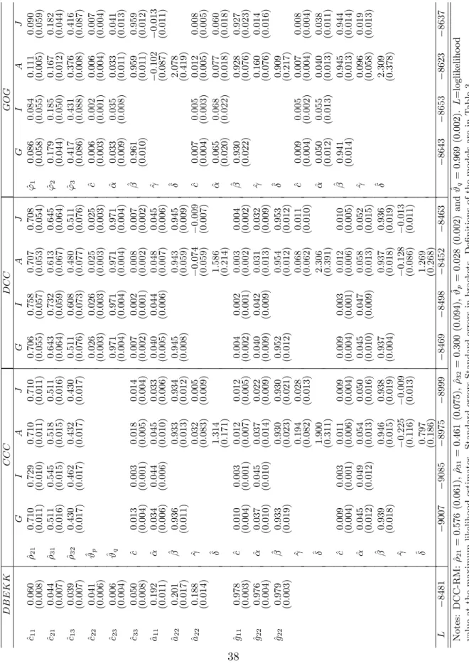
In the empirical application in Section 5, we consider 16 specifications forHmtwhich are frequently used in practice. As detailed in Section 4, for the simulation study, we consider a different forecasting models set (10 models), in order to control for the degree of similarity between models. The specifications considered in this paper are: diagonal BEKK (D-BEKK) model (Engle and Kroner, 1995), multivariate RiskMetrics model (J.P.Morgan, 1996), Con-stant Correlation (CCC) model (Bollerslev, 1990), Dynamic Conditional Correlation (DCC) model (Engle, 2002) and Generalized Orthogonal GARCH (GOG) model (van der Weide, 2002). The univariate GARCH specifications specifications for the conditional variance equa-tions used in the DCC, CCC and GOG are: GARCH (Bollerslev, 1986), GJR (Glosten, Jagannathan, and Runkle, 1992), Exponential GARCH (Nelson, 1991b), Asymmetric Power ARCH (Ding, Granger, and Engle, 1993), Integrated GARCH (Engle and Bollerslev, 1986), RiskMetrics (J.P.Morgan, 1996) and Hyperbolic GARCH (Davidson, 2004). Table 2 pro-vides a summary of the forecasting models set used in the simulation and the application respectively.
In the GJR model, the impact of squared innovations on the conditional variance is dif-ferent when the innovation is positive or negative. The asymmetric power ARCH model (APARCH) is a general specification which includes seven other ARCH extensions as special cases. The Exponential GARCH model (EGARCH) accommodates the asymmetric relation
Table 2: Forecasting models sets Simulation study
BEKK-type CCC GOG
Diag. BEKK GARCH GARCH
RiskMetrics IGARCH IGARCH
EGARCH EGARCH
RM HYGARCH
Note: Simulation based on bivariate models. CCC and GOG specifica-tion use the same condispecifica-tional variance specificaspecifica-tion for all series.
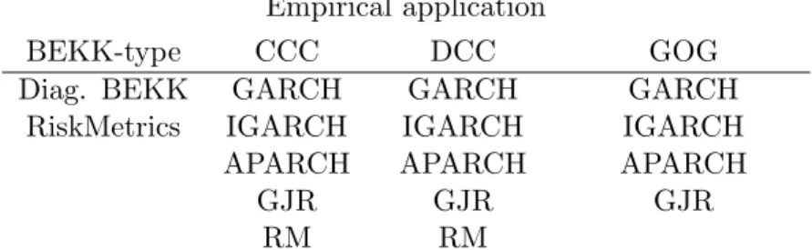
Empirical application
BEKK-type CCC DCC GOG
Diag. BEKK GARCH GARCH GARCH
RiskMetrics IGARCH IGARCH IGARCH
APARCH APARCH APARCH
GJR GJR GJR
RM RM
Note: Empirical application based on trivariate models. CCC, DCC and GOG specification use the same conditional variance specification for all series.
between shocks and volatility by expressing the latter as a function of both the magnitude and the sign of the shock. The Integrated GARCH (IGARCH) model is a variation of the GARCH model in which the sum of the ARCH and GARCH parameters are constrained to be equal to one, while the RiskMetrics model (RM) is basically an IGARCH model where the constant is set to zero and the ARCH and GARCH coefficients are fixed to 0.06 and 0.94 respectively. Finally, the Hyperbolic GARCH model (HYGARCH) allows to account for long run dependence in the volatility. The functional forms for Ht are briefly defined in Table 3. See Bauwens, Laurent, and Rombouts (2006) for further details. All the specifications are characterized by a constant conditional mean and the models are estimated by quasi maximum likelihood. The sample log-likelihood is given (up to a constant) by
−1 2 T t=1 log|Hm,t| −1 2 T t=1 (rt−μ)Hm,t−1(rt−μ), (15) whereT is the size of the estimation sample. We maximize numerically forμand the parame-ters inHm,t. All calculations and results reported in this paper are based on programs written by the authors using Ox version 6.0 (Doornik, 2002) and G@RCH version 6.0 (Laurent, 2009).
Table 3: Multivariate GARCH specifications
Model Multivariate GARCH models forHt (N = 2) # par.
DBEKK(1,1) Ht=C∗ 0 C0∗+A∗ t−1t−1A∗+G∗ Ht−1G∗ 7 RiskMetrics Ht= (1−α)t−1t−1+αHt−1, (α= 0.96) 0 GOG V−1/2 t=Lft 1+univ. Ht=V1/2LZtLV1/2 Zt=diag(σf12,t, . . . , σ2fm,t)
L=PΛ1/2U,U =i<jRi,j(δi,j),−π≤δi,j ≤π
CCC Ht=DtRDt 1+univ. Dt=diag(h11/,12,t. . . h1N,N,t/2 ) DCC(1,1) Ht=DtRtDt 3+univ. Rt=diag(q−1,11,t/2. . . qN,N,t−1/2)Qtdiag(q −1/2 1,1,t . . . qN,N,t−1/2) Dt=diag(h11/,12,t. . . h 1/2 N N t) ut=D−t1t Qt= (1−α−β) ¯Q+αut−1ut−1+βQt−1
Univariate GARCH models inZtandDt (l= 1,2)
GARCH(1,1) hl,t=ωl+αll,t2 −1+βlhl,t−1 6
EGARCH(1,0) log(hl,t) =ωl+g(zl,t−1) +βllog(hl,t−1) 8 g(zl,t−1) =θl,1zl,t−1+θl,2(|zl,t| −E(|zl,t|)) GJR(1,1) hl,t=ωl+αl2l,t−1+γlS−l,t−12l,t−1+βlhl,t−1 8 Sl,t− = 1 ifl,t<0;S−l,t= 0 ifl,t≥0 APARCH(1,1) hδl l,t=ωl+αl[|l,t−1| −γll,t−1]δl+βlhδl,tl−1 10 HYGARCH(1,d,1) hl,t=ωl[1−βl]−1+λ(L)2l,t 10 λ(L) =1−[1−βl]−1αl[1 +γl(1−L)d]
3.2 A proxy for the conditional variance matrix
Following Andersen, Bollerslev, Diebold, and Labys (2003), we rely on the realized covariance (RCov) to proxy the ex-post variance. In the ideal case of no microstructure noise, this measure, being based on intraday observations, is characterized by a degree of accuracy that decreases as sampling frequency lowers.
Let us assume the observed return vector to be generated by a conditionally normal N-dimensional log-price diffusion dy(u) and a N(N + 1)/2-dimensional covariance diffusion dσ(u), with σ(u) = vech(Σ(u)) = [σij(u)] for i, j = 1, ..., N, i ≥ j and u ∈ [t, t+ 1], with mean vector process b(u)du and variance matrix a(u) = s(u)s(u), driven by a N(N + 3)/2 vector of independent standard Brownian motions W(u). Hence the diffusion process of the system admits the following representation
⎡ ⎣ dy(u)
dσ(u) ⎤
⎦=b(u)du+s(u)dW(u), (16)
withb(u) ands(u) locally bounded and measurable. Consider now the following partition for the variance matrix of the system in (16) as
a(u) =s(u)s(u)= ⎡ ⎣ Σ(u) Cov(dy(u), dσ(u)) Cov(dy(u), dσ(u)) V ar(dσ(u)) ⎤ ⎦. (17)
Since Σ(u) identifies the continuous time process for the variance matrix of the returns, we can define the Integrated Covariance (ICov) as (see Barndorff-Nielsen and Shephard, 2004)
ICovt+1 = t+1
t
Σ(u)du. (18)
Let us now define the intraday returns asrt+Δ =yt+Δ−ytfort= Δ,2Δ, ..., T and where 1/Δ is the number of intervals per day. In this settingICovt can be consistently estimated by the Realized Covariance (RCov) (Andersen, Bollerslev, Diebold, and Labys, 2003) which is defined as RCovt+1,Δ= 1/Δ i=1 rt+iΔrt+iΔ. (19)
In fact, since the process defined by (16) does not allow for jumps in the returns, it holds that plim
In this paper, the RCov serves as a proxy for the true conditional variance matrix when evaluating the forecasting performance of the different MGARCH models. The result (20) suggests that the higher the intraday frequency used to computeRCov, and hence the amount of information available, the higher the accuracy of the proxy. The advantage of usingRCov is that it satisfies assumption A2.5 (see Barndorff-Nielsen and Shephard,2002 and Hansen and Lunde, 2006b) and therefore it ensures convergence of the approximated ordering to the true one under the inconsistent loss function (see Proposition 2). On the other hand,RCov is a valid proxy even when based on very low intraday sampling frequencies. The use of RCov allows to study the behavior of the ordering as a function of the level of accuracy of the proxy for consistent and inconsistent loss functions. As noted by Andersen, Bollerslev, Diebold, and Labys (2003), positive definiteness of the variance matrix is ensured only if the number of assets is smaller then 1/Δ. When this condition is violated then the realized covariance matrix fails to be of full rank (i.e.,rank(RCov) = 1/Δ< dim(RCov)) and RCov will meet only the weaker requirement to be semi-positive definite. Since the setting defined in this paper requires positive definiteness of the variance proxy, we restrict our analysis on the range of proxies that meet this requirement. Note that, other volatility proxies can be used instead, such as the multivariate realized kernels (see Barndorff-Nielsen, Hansen, Lunde, and Shephard, 2008a and Barndorff-Nielsen, Hansen, Lunde, and Shephard, 2008b, Hansen and Lunde, 2006b, Zhou, 1996) or the range based covariance estimators (Brandt and Diebold, 2006).
4
Simulation study
We investigate the ranking of the MGARCH models with respect to two dimensions: the quality of the volatility proxy and the choice of the loss function. According to Proposition 2, we find that if the quality of the proxy is sufficiently good, both consistent and inconsistent loss functions rank properly. However, when the quality of the proxy is poor, only the consistent loss functions rank correctly. Our findings also hold when the sample size in the estimation period increases.