Scaling a convolutional neural network for classification of adjective noun pairs with TensorFlow on GPU clusters

Scaling a Convolutional Neural Network for

classification of Adjective Noun Pairs with

TensorFlow on GPU Clusters

V´ıctor Campos

, Francesc Sastre

, Maurici Yag¨ues

, Jordi Torres

and Xavier Gir´o-i-Nieto

{victor.campos, jordi.torres, francesc.sastre, maurici.yagues, jordi.torres}@bsc.es †_{Universitat Polit`ecnica de Catalunya, UPC Barcelona Tech}

[email protected] Abstract—Deep neural networks have gained popularity in

recent years, obtaining outstanding results in a wide range of applications such as computer vision in both academia and multiple industry areas. The progress made in recent years cannot be understood without taking into account the technological advancements seen in key domains such as High Performance Computing, more specifically in the Graphic Processing Unit (GPU) domain. These kind of deep neural networks need massive amounts of data to effectively train the millions of parameters they contain, and this training can take up to days or weeks depending on the computer hardware we are using. In this work, we present how the training of a deep neural network can be parallelized on a distributed GPU cluster. The effect of distributing the training process is addressed from two different points of view. First, the scalability of the task and its performance in the distributed setting are analyzed. Second, the impact of distributed training methods on the training times and final accuracy of the models is studied. We used TensorFlow on top of the GPU cluster of servers with 2 K80 GPU cards, at Barcelona Supercomputing Center (BSC). The results show an improvement for both focused areas. On one hand, the experiments show promising results in order to train a neural network faster. The training time is decreased from 106 hours to 16 hours in our experiments. On the other hand we can observe how increasing the numbers of GPUs in one node rises the throughput, images per second, in a near-linear way. Moreover an additional distributed speedup of 10.3 is achieved with 16 nodes taking as baseline the speedup of one node.

Keywords—Distributed Computing; Parallel Systems; Deep Learning; Convolutional Neural Networks; Computer Vision; Graphic Processing Unit; TensorFlow

I. OVERVIEW OF THE PROBLEM

Methods based on deep neural networks have established the state-of-the-art in computer vision tasks [16], [24], [10].

Although the development of these algorithms spans over many decades [17], their potential has been unlocked by the increased computational power of specific accelerators, e.g. Graphical Processing Units (GPUs), and the creation of large-scale datasets [9], [14]. Even with the use of specific hardware devices, training these algorithms is so computation-ally intensive that can take days, or even weeks, to converge on a single machine.

Distributed and parallel computing has emerged as an efficient solution for tackling growing deep learning

chal-lenges. These platforms allow the scalability of machine learning tasks, enabling some properties that could not be achieved with single-machine processing. However, scaling up the computation to a distributed system is also a more difficult task than working on a single machine. Depending on the efficiency of the algorithm, communication between nodes can be a bottleneck, and the system has to be robust in order to overcome possible failures.

For this work we use a special application of Convolutional Neural Networks (CNN) called Affective Computing [22] that has recently garnered much research attention. Machines that are able to understand and convey subjectivity and affect would lead to a better human-computer interaction that is key in some fields such as robotics or medicine. Despite the success in some constrained environments such as emotional understanding of facial expressions [19], automated affect understanding in unconstrained domains remains an open challenge which is still far from other tasks where machines are approaching or have even surpassed human performance. In this work, we will focus on the detection of Adjective Noun Pairs (ANPs) using a large-scale image dataset collected from Flickr [13]. These mid-level representations, which are a rising approach for overcoming the affective gap between low level image features and high level affect semantics, can then be used to train accurate models for visual sentiment analysis or visual emotion prediction.

As a framework we used TensorFlow [2]. TensorFlow sup-ports large-scale training and inference in multiple platforms and architectures, and aims to be a flexible framework for both experimenting and running in production environments. This is achieved by using dataflow programming models (Spark, MapReduce, COMPSs) which provide a number of useful abstractions that insulate from low level details of distributed processing. Then, communication between subcomputations is explicit and makes it easy to partition and run independent sub-graphs on multiple distributed devices.

The massive number of convolutions and matrix multipli-cations in neural networks has led to GPU implementations with CUDA [21] and efficient, task specific primitives using cuDNN [8]. Early deep learning frameworks such as Caffe [11] or Theano [4] provided fast and easy access to such primitives, but were initially designed for single machine operation, without support for distributed environments. Efforts © 2017 IEEE. Personal use of this material is permitted. Permission from IEEE must be obtained for all other uses, in any current or future media, including reprinting/republishing this material for advertising or promotional purposes,creating new collective works, for resale or redistribution to servers or lists, or reuse of any copyrighted component of this work in other works.

towards distributing the former frameworks with traditional HPC tools such as Spark or MPI resulted in projects such as SparkNet [20] or Theano-MPI [18]. Native support for distributed settings is included in more recent frameworks such as TensorFlow [2], MXNet [7] or CNTK [27]. However, scaling the training algorithms from a single machine environ-ment to a distributed setting poses two main challenges. From the computing performance standpoint, optimizing the use of resources is the main goal, whereas from the learning side, the final accuracy should not suffer a drop when compared to its single machine counterpart.

In this work, we explore how the training of CNNs for ANP classification can be accelerated through distribution in a GPU cluster. Two main approaches are proposed in the literature [15] to train CNNs on a multi-GPU environment, either in a single machine or in a distributed setting: model parallelism and data parallelism. Model parallelism splits layers in the CNN among different GPUs, i.e. each GPU operates over the same batch of input data, but applying different operations on them, and is mostly used for operations with a large number of parameters that may not fit in the GPU’s memory. On the other hand, data parallelism consists in placing a replica of the model on each GPU, which then operates on a different batch of data. Model replicas share parameters, so that this method is equivalent to having a larger batch size. Given the topology of modern CNN architectures and current hardware characteristics, we will consider multi-GPU data parallelism for both single machine and distributed settings.

Our contributions are three-fold: (1) we study the trade-off between final classification accuracy and speedup and analyze the results both from the learning and HPC standpoints, (2) distribute the training in a way that makes the most of the clus-ter resources, leveraging intra-node and inclus-ter-node parallelism, and (3) propose a modification of the distributed configuration, in order to reduce the resources being used while training.

II. PROBLEM BEING SOLVED: ADJECTIVENOUNPAIRS A. Dataset

We use a specific application of CNN called Adjective Noun Pairs (ANPs). These are powerful mid-level represen-tations [5] that can be used for affect related tasks such as visual sentiment analysis or emotion recognition. A large-scale ANP ontology for 12 different languages, namely Multilingual Visual Sentiment Ontology (MVSO), was collected by Jou et al. [13] following a model derived from psychology studies, Plutchick’s Wheel of Emotions [23]. The noun component in an ANP can be understood to ground the visual appearance of the entity, whereas the adjective polarizes the content towards a positive or negative sentiment, or emotion [13]. These properties try to bridge the affective gap between low level image features and high level affective semantics, which goes far beyond recognizing the main object in an image. Whereas a traditional object classification algorithm may recognize a baby in an image, a finer-grained classification such ashappy baby or crying baby is usually needed to fully understand the affective content conveyed in the image. Capturing the sophisticated differences between ANPs poses a challenging task that requires from high capacity models and large-scale annotated datasets.

In our experiments we consider a subset of the English par-tition of MVSO, the tag-restricted subset, which contains over 1.2M samples covering 1,200 different ANPs. Since images in MVSO were downloaded from Flickr and automatically annotated using their metadata, such annotations have to be considered asweak labels, i.e. some labels may not match the real content of the images. The tag-pool subset contains those samples for which the annotation was obtained from the tags in Flickr instead of other metadata, so that annotations are more likely to match the real ground truth.

B. CNN architecture

Since the first successful application of CNNs to large-scale visual recognition, the design of improved architectures for improved classification performance has focused on increasing the depth, i.e. the number of layers, while keeping or even reducing the number of trainable parameters. This trend can be seen when comparing the 8 layers in AlexNet [16], the first CNN-based method to win the Image Large Scale Visual Recognition Challenge (ILSVRC), with the dozens, or even hundreds, of layers in Residual Nets (ResNets) [10]. Despite the huge increase in the overall depth, a ResNet with 50 layers has roughly half the parameters in AlexNet. However, the impact of an increased depth is more notorious in the memory footprint of deeper architectures, which store more intermediate results coming from the output of each single layer, thus benefiting from multi-GPU setups that allow the use of larger batch sizes.

We adopt the ResNet50 CNN [10] on our experiments, an architecture with 50 layers that maps a 224×224×3 input image to a 1,200-dimensional vector representing a probability distribution over the ANP classes in the dataset. Overall, the model contains over 25×106 _{single-precision floating-point}

parameters involved in over 4×109 _{floating-point operations}

that are tuned during training. It is important to notice that the more computationally demanding a CNN is, the larger the gains of a distributed training due to the amount of time spent doing parallel computations with respect to the added communication overhead.

Cross-entropy between the output of the CNN and the ground truth, i.e. the real class distribution, is used as loss function together with an L2 regularization term with a weight decay rate of 10−4_{. The parameters in the model are tuned}

to minimize the former cost objective using batch gradient descent.

III. IMPLEMENTED NEURAL NETWORK ARCHITECTURE A. Distributed Neural Network training

The process of training CNNs with batch gradient descent can be decomposed in two main steps: forward and backwards passes through the net. Theforward passcomputes the outputs for a batch of data, and an error with respect to the desired result is then calculated. Such error, or cost, is then differ-entiated with respect to every parameter in the CNN during the so called backwards pass. Finally, the resulting gradients are used to update the weights in the net. These steps are iteratively repeated until convergence, i.e. until a local minima in the error function is reached.

In this implementation we use the data parallelism paradigm, in which we define two kind of nodes. First, the worker nodes each has a replica of the model, operating on separate batches of data. Second, the parameter server (PS) nodes store and update the model parameters [1]. In essence, the worker will receive the model parameters, compute it on a batch of data, and send back the gradients to the PS where the model will be updated in order to improve it [6].

B. TensorFlow strategies

TensorFlow enables multiple strategies for aggregating the results in multinode settings when working with data paral-lelism:

Synchronous mode: In this case, the PS waits until all worker nodes have computed the gradients with respect to their data batches. Once the gradients are received by the PS, they are applied to the current weights and the updated model is sent back to all the worker nodes. This method is as fast as the slowest node, as no updates are performed until all worker nodes finish the computation, and may suffer from unbalanced network speeds when the cluster is shared with other users. However, faster convergence is achieved as more accurate gradient estimations are obtained. Authors in [6] present an alternative strategy for alleviating the slowest worker update problem by using backup workers.

Asynchronous mode: every time the PS receives the gradients from a worker, the model parameters are updated. Despite delivering an enhanced throughput, compared to its synchronous counterpart, every worker may be operating on a slightly different version of the model, thus providing poorer gradient estimations. As a result, more iterations are required until convergence due to the stale gradient updates. Increasing the number of workers, may result in a throughput bottleneck by the communication with the PS, in which case more PS need to be added.

Mixed mode: mixed mode appears as a trade-off be-tween adequate batch size and throughput by performing asynchronous updates on the model parameters, but using synchronously averaged gradients coming from subgroups of workers. Larger learning rates can be used thanks to the increased batch size, leading to a faster convergence, while reaching throughput rates close to those in the asynchronous mode.

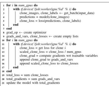
C. Implemented Architecture: Mixed asynchronous mode As seen in the previous case, having multiple GPUs on the same server implies some constraints when building our distributed models. The mixed asynchronous mode is more suited for our architecture, as we can use synchronous mode between GPUs on the same node, and asynchronously update the model between servers. In other words, we are using synchronous replicas intra-node and asynchronous replicas inter-node. However, deploying the model and gathering the statistics in each GPU is more complex than the previous mode, because device placement needs to be done at the code level manually which adds complexity to the overall process. In the cluster definition each worker will have 4 available GPUs, so we will only have a worker for each node. Figure 1

CUDA_VISIBLE_DEVICES="" python script.py \ --ps_hosts=nvb1-ib0:2220 \

--worker_hosts=nvb1-ib0:2221 \ --job_name=ps --task_index=0 & \

CUDA_VISIBLE_DEVICES="0,1,2,3" python script.py \ --ps_hosts=nvb1-ib0:2220 \

--worker_hosts=nvb1-ib0:2221 \ --job_name=worker --task_index=0

Fig. 1: Distributed call for PS and worker

1 foriinnum gpusdo

2 withtf.device(’/job:worker/gpu:%d’ % i)do

3 clone images, clone labels←get batch(input data) 4 predictions = model(clone images)

5 clone loss = loss(predictions, clone labels)

6 end 7 end

8 grad op←create optimizer

9 grads and vars, clone losses←create empty lists

10 foriinnum gpusdo

11 withtf.device(’/job:worker/gpu:%d’ % i)do 12 clone loss = get loss for clonei

13 scaled clone loss = clone loss / num gpus

14 clone grad = compute gradients wrt trainable variables 15 append clone grad to grads and vars

16 append scaled clone loss to clone losses

17 end 18 end

19 total loss = sum clone losses 20 total gradients = sum grads and vars

21 update the model with total gradients

Algorithm 1:Clone allocation and gradient computation

shows how the call will look like, for allocating a single PS and a single worker in a unique node.

This worker will have all 4 GPUs available, and the model will be responsible for placing the clones in the corresponding GPU. The function for enforcing device placement constraints in TensorFlow is tf.device(), and we can specify a loop to place the model to all available GPUs. This process will be again replicated to multiple nodes using the

tf.train.replica_device_setter, and the total number of GPUs used will be the same. The key difference in this method is the way gradients are aggregated among all the clones in the node, which will make the iteration with a bigger effective size batch.

The pseudocode in Algorithm 1 aims to provide a general understanding of the main part of the mixed asynchronous procedure that places and computes the model in the 4 GPUs available, collects the losses and gradients in each one and reports it back to the PS.

IV. EXPERIMENTAL SETUP A. Platform

We evaluate our experiments in the GPU cluster Minotauro. This is a heterogeneous cluster with 2 configurations, although TensorFlow installation only works on servers installed with NVIDIA K80, and not on the older servers with NVIDIA M2090. Therefore the cluster configuration we use has 39 bullx R421-E4 servers, each server with [3]:

• 2 Intel Xeon E5-2630 v3 (Haswell) 8-core processors (at 2.4 GHz, 20MB L3 cache)

• 2 K80 NVIDIA GPU Cards

• 128 GB of Main memory, distributed in 8 DIMMs of 16 GB - DDR4 @ 2133 MHz - ECC SDRAM

• Peak Performance: 250.94 TFlops

• 1 PCIe 3.0 x8 8GT/s, Mellanox ConnectXR - 3FDR 56 Gbit

• 4 Gigabit Ethernet ports B. Software Middleware

The operating system is RedHat Linux 6.7. The CNN archi-tectures and their training are implemented with TensorFlow1 version 0.11.0 RC0 , running on CUDA 7.5 and using cuDNN 5.1.3 primitives for improved performance. Since the train-ing process needs to be submitted through Slurm Workload Manager, task distribution and communication between nodes is achieved with Greasy2_{. Unlike other publications, where} each worker is defined as a single GPU [6], [12], we use all available GPUs in each node to define a single worker. Given the dual nature of the NVIDIA K80 cards, four model replicas are placed in each node.

As discussed before, the mixed approach is selected for the setup. This setup offers two main advantages: (1) all GPUs in each node are used, which minimizes communication overhead, as only a single collection of gradients needs to be exchanged through the network for each set of four model replicas, and (2) each worker has larger effective batch size, providing better gradient estimations and allowing the use of larger learning rates for faster convergence.

The loss function is minimized using RMSProp [25] per-parameter adaptive learning rate as optimization method with a learning rate of 0.1, decay of 0.9 and = 1.0. To prevent overfitting, data augmentation consisting in random crops and/or horizontal flips is asynchronously performed on CPU while previous batches are processed by the GPUs. The CNN weights are initialized using a model pre-trained on ILSVRC [9], practice that has been proven beneficial even when training on large-scale datasets [26].

C. Resource efficiency

Available publications on distributed training with Tensor-Flow [1], [6] tend to use different server configurations for worker and PS tasks. Given the PS only stores and updates the model and there is no need for GPU computations, only CPU servers are used for this task. On the other hand, most of the worker job involves matrix computations, for which servers equipped with GPUs are used. Our configuration imposes some constraints, as we only have GPU equipped nodes, which means that placing PS and workers in different nodes will result in under-utilization of GPU resources. We decided to study the impact of placing the PS in the same nodes as the workers, and restricting the resource usage in each task. We used odd values of PS, because variables are sharded using a

1_{https://www.tensorflow.org/} 2_{https://github.com/jonarbo/GREASY}

round-robin strategy. Since the weights of the layers take much of the model size, and layer weights and bias are initialized consecutively, we want to have them as much distributed as possible, hence the use of an odd value.

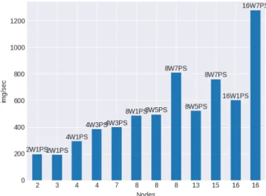
Fig. 2: Throughput comparison between different distributed setups

Figure 2 shows different configurations of worker and PS setups with their respective throughput. With these results, it seems that the cluster configuration can cope with workers and PS in the same node, as throughputs are quite similar when placing PS inside or outside the worker nodes. However, a more important task is to correctly tune the amount of PS needed so as to not have a network or server bottleneck. In addition, when placing PS with workers, we place them on workers that need not to run auxiliary tasks of the training, such as checkpoint saving or summary writing, in order to not overload the CPU.

V. RESULTS AND DISCUSSION A. GPU parallelism

Tensorflow enables us to assign different tasks to the available resources of a node (CPU and GPUs). In order to make use of all available resources in a node, we put a network clone in each GPU. The NVDIA K80, as discused before, can work as two GPUs and has enough memory to hold two clones. With these, we could do data parallelism using batches of 32 images per clone (128 images per node).

In Figure 3a, we can observe how increasing the number of GPUs rises the throughput, increasing the images per second processed, in a near-linear way. This parallelism inside a node is made entirely synchronous, in each training iteration the CPU waits for all GPUs and merges the obtained gradients to start a new iteration. We will use this method inside each node in order to reduce the network usage.

B. Speedup (throughput)

In this case, we are doing the mixed-asynchronous ap-proach. The gradients of each GPU are combined at the node, and are later sent to the parameter server.

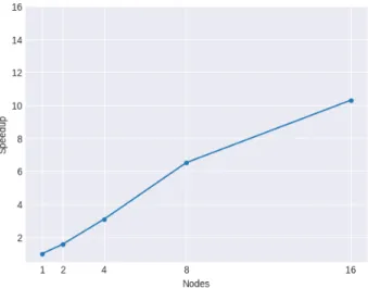
(a) Parallelism speedup inside a node using different number of GPUs.

(b) Distribution speedup using several nodes, with 4 GPUs, with the optimal configuration. The baseline is one node with 4 GPUs.

Fig. 3: Throughput speedup in a node and with different setups.

Setup Throughput Speedup Efficiency 1 Node (No distribution) 124.18 img/sec - -2 Nodes (-2 Workers + 1 PS) 195.60 img/sec 1.58 0.79 4 Nodes (4 Workers + 3 PS) 383.09 img/sec 3.09 0.77 8 Nodes (8 Workers + 7 PS) 809.10 img/sec 6.52 0.82 16 Nodes (16 Workers + 7 PS) 1278.53 img/sec 10.30 0.64 TABLE I: Speedup comparing a single node between different distributed configurations and their speedup-resources relation.

For example, with eight nodes, we dispose of 32 GPUs. In a pure asynchronous strategy, the training process would need to send 32 model gradients through the network to the parameters servers, and then retrieve the updated model that can have around 400 MB. The whole process could need 12 GB for each iteration, which might cause overhead in the network and penalize the overall throughput. In the mixed approach, we try to reduce the network overhead reducing by four the data transfer doing only one sending of data per node.

Table I shows a brief detail about the throughput and the speedup among different setups. It is important to note the decrease in efficiency as the number of nodes grows, that is also related in diminishing return at training times. In Figure 3b there is a throughput comparison between all the tested configurations. We discern an improvement, although it is not linear, because there are a higher amount of resources to process and send through the network.

C. Speedup (from the learning standpoint)

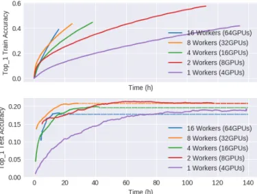
At the top of Figure 4 we can see the evolution of the training accuracy, and notice how multi-node configuration can reach similar accuracy values much faster than using a single-node setup. However, the performance gains are reduced as more nodes are added to the computation, due to the use of more resources and the higher amount of stale gradients.

Bottom part of Figure 4 shows how the test accuracy evolves and converges. In Table II we can see the amount of time different configurations spent arriving at the maximum accuracy. It is important to highlight the improvement in training time among the multiple configurations, although with diminishing returns.

Test accuracy results are not as good as the single node configuration, but given that we have not optimized hyperpa-rameters for distributed training, and we focused on scalability with multiple nodes, a further analysis should be made (pres-ence of stale gradients, hyperparameter tuning, etc.) in order to understand these results.

Workers (GPUs) Test Accuracy Time (h) Improvement 1 Node (4) 0.228 106.43 1.00 2 Nodes (8) 0.217 62.78 1.69 4 Nodes (16) 0.202 37.99 2.80 8 Nodes (32) 0.217 22.50 4.73 16 Nodes (64) 0.185 16.49 6.45

TABLE II: Reached accuracy, spent time and improvement range among the optimal setups.

VI. CONCLUSION

Distributed training strategies for deep learning architec-tures will become more important as the size of datasets in-creases. Therefore, it is important to identify the most efficient ways to perform distributed training, in order to maximize the throughput of the system, while minimizing the accuracy decrease.

We have used the mixed-asynchronous mode because it is more network efficient than the fully asynchronous mode, and we showed that the speedup inside a worker scales up better than when scaling to multiple nodes due to the effect of network overhead.

From the throughput standpoint, Figure 3b shows a near-linear increase and a resource usage near to 80%. There is a degradation in the 16 node experiment, and it may be due to external factors like network overhead.

We managed to decrease the training times from 106 hours to 16 hours (more than 6 times less), albeit with some accuracy loss. There are different results depending on the number of

Fig. 4: Top: Train accuracy evolution in different distributed configurations. Bottom:Test accuracy evolution until conver-gence in different distributed configurations.

nodes, and this solution is adaptable to clusters of different sizes and configurations, number of nodes or GPUs per node. When we looked for the best configuration for each num-ber of workers, we found that the best throughput-resources relation was: 2 workers and 1 PS in 2 nodes, 4 workers and 3 PS in 4 nodes, 8 workers and 7 PS in 8 nodes and 16 workers and 7 PS in 16 nodes.

ACKNOWLEDGEMENTS

This work is partially supported by the Spanish Ministry of Economy and Competitivity under contract TIN2012-34557, by the BSC-CNS Severo Ochoa program (SEV-2011-00067), by the SGR programmes (1051 and 2014-SGR-1421 ) of the Catalan Government and by the framework of the project BigGraph TEC2013-43935-R, funded by the Spanish Ministerio de Economia y Competitividad and the European Regional Development Fund (ERDF). We also would like to thank the technical support team at the Barcelona Supercom-puting center (BSC) especially to Carlos Tripiana.

REFERENCES

[1] M. Abadi, P. Barham, J. Chen, Z. Chen, A. Davis, J. Dean, M. Devin, S. Ghemawat, G. Irving, M. Isard, M. Kudlur, J. Levenberg, R. Monga, S. Moore, D. G. Murray, B. Steiner, P. Tucker, V. Vasudevan, P. Warden, M. Wicke, Y. Yu, and X. Zheng. TensorFlow: A system for large-scale machine learning. ArXiv e-prints, May 2016.

[2] Martın Abadi, Ashish Agarwal, Paul Barham, Eugene Brevdo, Zhifeng Chen, Craig Citro, Greg S Corrado, Andy Davis, Jeffrey Dean, Matthieu Devin, et al. Tensorflow: Large-scale machine learning on heteroge-neous systems. 2015.

[3] Barcelona Supercomputing Center (BSC). Minotauro user’s guide, 2017.

[4] James Bergstra, Fr´ed´eric Bastien, Olivier Breuleux, Pascal Lam-blin, Razvan Pascanu, Olivier Delalleau, Guillaume Desjardins, David Warde-Farley, Ian Goodfellow, Arnaud Bergeron, et al. Theano: Deep learning on gpus with python. InNIPS Workshops, 2011.

[5] Damian Borth, Rongrong Ji, Tao Chen, Thomas Breuel, and Shih-Fu Chang. Large-scale visual sentiment ontology and detectors using adjective noun pairs. InACM MM, 2013.

[6] Jianmin Chen, Xinghao Pan, Rajat Monga, Samy Bengio, and Rafal Jozefowicz. Revisiting Distributed Synchronous SGD. ICLR 2017 conference submission, 2016.

[7] Tianqi Chen, Mu Li, Yutian Li, Min Lin, Naiyan Wang, Minjie Wang, Tianjun Xiao, Bing Xu, Chiyuan Zhang, and Zheng Zhang. Mxnet: A flexible and efficient machine learning library for heterogeneous distributed systems. arXiv preprint arXiv:1512.01274, 2015. [8] Sharan Chetlur, Cliff Woolley, Philippe Vandermersch, Jonathan Cohen,

John Tran, Bryan Catanzaro, and Evan Shelhamer. cudnn: Efficient primitives for deep learning. arXiv preprint arXiv:1410.0759, 2014. [9] Jia Deng, Wei Dong, Richard Socher, Li-Jia Li, Kai Li, and Li Fei-Fei.

ImageNet: A large-scale hierarchical image database. InCVPR, 2009. [10] Kaiming He, Xiangyu Zhang, Shaoqing Ren, and Jian Sun. Deep

residual learning for image recognition. InCVPR, 2016.

[11] Yangqing Jia, Evan Shelhamer, Jeff Donahue, Sergey Karayev, Jonathan Long, Ross Girshick, Sergio Guadarrama, and Trevor Darrell. Caffe: Convolutional architecture for fast feature embedding. In ACM MM, 2014.

[12] Peter H Jin, Qiaochu Yuan, Forrest Iandola, and Kurt Keutzer. How to scale distributed deep learning? arXiv preprint arXiv:1611.04581, 2016.

[13] Brendan Jou, Tao Chen, Nikolaos Pappas, Miriam Redi, Mercan Top-kara, and Shih-Fu Chang. Visual affect around the world: A large-scale multilingual visual sentiment ontology. InACM MM, 2015.

[14] Andrej Karpathy, George Toderici, Sanketh Shetty, Thomas Leung, Rahul Sukthankar, and Li Fei-Fei. Large-scale video classification with convolutional neural networks. InCVPR, 2014.

[15] Alex Krizhevsky. One weird trick for parallelizing convolutional neural networks. arXiv preprint arXiv:1404.5997, 2014.

[16] Alex Krizhevsky, Ilya Sutskever, and Geoffrey E. Hinton. ImageNet classification with deep convolutional neural networks. InNIPS, 2012. [17] Yann LeCun, L´eon Bottou, Yoshua Bengio, and Patrick Haffner. Gradient-based learning applied to document recognition.Proceedings of the IEEE, 86(11), 1998.

[18] He Ma, Fei Mao, and Graham W Taylor. Theano-mpi: a theano-based distributed training framework.arXiv preprint arXiv:1605.08325, 2016. [19] Daniel McDuff, Rana El Kaliouby, Jeffrey F Cohn, and Rosalind W Picard. Predicting ad liking and purchase intent: Large-scale analysis of facial responses to ads. IEEE Transactions on Affective Computing, 6(3), 2015.

[20] Philipp Moritz, Robert Nishihara, Ion Stoica, and Michael I Jor-dan. Sparknet: Training deep networks in spark. arXiv preprint arXiv:1511.06051, 2015.

[21] CUDA Nvidia. Compute unified device architecture programming guide. 2007.

[22] Rosalind W. Picard. Affective Computing, volume 252. MIT Press Cambridge, 1997.

[23] Robert Plutchik. Emotion: A Psychoevolutionary Synthesis. Harper & Row, 1980.

[24] Christian Szegedy, Wei Liu, Yangqing Jia, Pierre Sermanet, Scott Reed, Dragomir Anguelov, Dumitru Erhan, Vincent Vanhoucke, and Andrew Rabinovich. Going deeper with convolutions. InCVPR, 2015. [25] Tijmen Tieleman and Geoffrey Hinton. Lecture 6.5-rmsprop: Divide the

gradient by a running average of its recent magnitude. COURSERA: Neural Networks for Machine Learning, 4, 2012.

[26] Jason Yosinski, Jeff Clune, Yoshua Bengio, and Hod Lipson. How transferable are features in deep neural networks? InNIPS, 2014. [27] Dong Yu and Xuedong Huang. Microsoft Computational Network