Assessing macro uncertainty in real-time when data are subject to revision

Assessing macro uncertainty in real­time 

when data are subject to revision 

Article 

Accepted Version 

Clements, M. P. (2017) Assessing macro uncertainty in real­

time when data are subject to revision. Journal of Business & 

Economic Statistics, 35 (3). pp. 420­433. ISSN 0735­0015 doi: 

https://doi.org/10.1080/07350015.2015.1081596 Available at 

http://centaur.reading.ac.uk/41466/ 

It is advisable to refer to the publisher’s version if you intend to cite from the 

work. 

To link to this article DOI: http://dx.doi.org/10.1080/07350015.2015.1081596 

Publisher: Taylor & Francis 

All outputs in CentAUR are protected by Intellectual Property Rights law, 

including copyright law. Copyright and IPR is retained by the creators or other 

copyright holders. Terms and conditions for use of this material are defined in 

the 

End User Agreement  

. 

www.reading.ac.uk/centaur  

CentAUR 

Assessing Macro Uncertainty In Real-Time

When Data Are Subject To Revision

Michael P. Clements ICMA Centre Henley Business School

University of Reading m.p.clements@reading.ac.uk

August 6, 2015

Abstract

Model-based estimates of future uncertainty are generally based on the in-sample …t of the model, as when Box-Jenkins prediction intervals are calculated. However, this approach will generate biased uncertainty estimates in real time when there are data revisions. A simple remedy is suggested, and used to generate more accurate prediction intervals for 25 macroeconomic variables, in line with the theory. A simulation study based on an empirically-estimated model of data revisions for US output growth is used to investigate small-sample properties.

Keywords: in-sample uncertainty, out-of-sample uncertainty, real-time-vintage estima-tion

JEL code: C53.

Michael P. Clements is an Associate member of the Institute for New Economic Thinking, Oxford Martin School, University of Oxford, UK.

Assessing Macro Uncertainty In Real-Time

When Data Are Subject To Revision

Model-based estimates of future uncertainty are generally based on the in-sample …t of the model, as when Box-Jenkins prediction intervals are calculated. However, this approach will generate biased uncertainty estimates in real time when there are data revisions. A simple remedy is suggested, and used to generate more accurate prediction intervals for 25 macroeconomic variables, in line with the theory. A simulation study based on an empirically-estimated model of data revisions for US output growth is used to investigate small-sample properties.

Keywords: in-sample uncertainty, out-of-sample uncertainty, real-time-vintage esti-mation

1

Introduction

There has been much recent interest in macro-forecasting in real-time. By this we mean how the forecasting model should be speci…ed, estimated, and the resulting forecasts evaluated, once we acknowledge that the data on which these three activities is based is subject to revision (for all but a small number of series such as interest rates and exchange rates). A number of papers have considered modelling the revisions process (see, e.g., Cunningham, Eklund, Je¤ery, Kapetanios and Labhard (2009), Jacobs and van Norden (2011), Kishor and Koenig (2012)); or using single-equation models with ‘real-time-vintages’ (as in Koenig, Dolmas and Piger (2003), Clements and Galvão (2013b)) which we refer to as RTV-estimation and discuss below; or modelling multiple vintages of data, as with vintage-based vector autoregressive models (see, e.g., Patterson (1995, 2003), Clements and Galvão (2013a)). Other papers have considered whether assessing predictability in real-time may change the conclusions one would draw concerning putative explanatory forces, or the usefulness of estimates of the output gap as a guide to monetary policy in real time. On the former, it has been argued that the use of …nal-revised data may exaggerate the predictive power of explanatory variables relative to what could actually have been achieved at the time using the then available data (see, e.g., Robertson and Tallman (1998), Faust, Rogers and Wright (2003)), and on the latter see Orphanides (2001), Orphanides and van Norden (2005), Garratt, Lee, Mise and Shields (2009, 2008) and Clements and Galvão (2012),inter alia. Croushore (2011a, 2011b) provide useful state-of-the-art reviews. These related strands of research are all concerned with …rst-moment prediction: either improving the accuracy of forecasts of the conditional expectation, or of providing a more realistic appraisal of the accuracy of these predictions. In this paper we instead investigate the implications of data revisions for assessments of forecast uncertainty, speci…cally, the accuracy of prediction intervals. We show that the ‘traditional’ approaches to calculating prediction intervals will tend to be either too wide, when data revisions ‘add news’, or too narrow, when the revisions process ‘removes noise’. The standard approach is due to Box-Jenkins (Box and Jenkins (1970)). The e¤ects of data vintages in real-time analyses are …rst-order, in the sense that they do not disappear when the sample size gets large, and are not caused by non-normal errors. It is recognized in the literature that Box-Jenkins prediction intervals su¤er from the neglect of parameter estimation uncertainty and the possible non-normality of the underlying

model’s disturbances, and as a result there has been much interest in bootstrapping prediction intervals (see e.g., Thombs and Schucany (1990)). Yet we show that in real-time prediction intervals will have incorrect coverage even in the absence of these problems (i.e., in the absence of parameter estimation uncertainty, and when the disturbances are normal), because of data vintage e¤ects. We use simple Box-Jenkins intervals to focus on data vintage e¤ects.

Clearly, the e¤ects of data vintages on …rst and second-moment prediction can be side-stepped by considering fully-revised data, whence observations are no longer subject to revision. Of course any observation no matter how far back in time may be changed in response to far-reaching methodological changes. By fully-revised data we mean data that have undergone the initial and three annual rounds of revisions (see e.g., Landefeld, Seskin and Fraumeni (2008) for a description of the revisions process of the US Bureau of Economic Analysis NIPA data). Pseudo out-of-sample exercises use fully-revised data (e.g., the vintage of data available at the time of the study), and at each point in time the forecasting models are speci…ed and the parameters estimated using only data for time periods up to that point in time. Such exercises are useful as a way of assessing how well the model or models …t or forecast the true data, and the out-of-sample aspect guards against ‘over…tting’, i.e., the models capturing chance or non-recurrent sample-speci…c features. A real-time forecasting exercise mimics the environment a real-world forecaster faces - at each point in time the forecasting models are speci…ed and the parameters estimated using only data for time periods up to that point in time, but in addition the data are taken from the vintages that would have been available at that point in time. Real-time exercises are required to provide fair assessments of the relative accuracy of the model forecasts compared to survey expectations, for example.

To illustrate, assume a one period delay in data availability. Then at timeta forecaster will have access to the vintage-t value of the period t 1 observation, denoted y_tt ₁, and similarly the second estimate of the t 2 period, yt_{t 2}, and so on. If the forecaster wishes to use only data which has been revised n times, say, the most recent data that could be used would be for t n 1 (i.e., y_{t n}t ₁, y_{t n}t ₂; : : :). It will rarely be optimal to ignore data for periods

t n 2; : : : ; t 1 (for large n), so the real-world forecaster will be forced to work with data subject to revision. This is the environment we seek to mimic in the real-time analysis.

is a zero-mean …rst-order autoregressive process (AR(1)), and the true value of the process is revealed the period after the …rst estimate, so only the …rst estimate is subject to revision. Further, we ignore estimation uncertainty, so that model parameters take on their population parameters. We show that the standard approach gives an incorrect assessment of forecast uncertainty, and consequently incorrectly-sized prediction intervals. We focus on prediction intervals, but the points we make apply more generally to measures of forecast uncertainty (such as forecast densities). In section 3 we broaden the analysis of section 2 to an AR(p)

for the true process, and allow a general revisions process with multiple revisions. As in the simple case, there will in general be a misleading assessment of the uncertainty surrounding future outcomes. We then suggest a remedy that has been used for …rst-moment prediction, and has the virtue of simplicity and does not require that the revisions process be modelled: section 4. Section 5 supposes the goal is to estimate the uncertainty about future revised values, as opposed to …rst-release data. Section 6 provides an empirical illustration, and shows the improvements that result from using the approach advocated in this paper. We consider 25 macro variables, which exhibit di¤erent patterns of revisions, so that the conclusions we draw are reasonably general and do not rest on a few variables with (possibly) idiosyncratic features. In section 7 we present a simulation study of the two approaches to calculating prediction intervals in a controlled environment that abstracts from various factors that might a¤ect the empirical comparisons, such as parameter non-constancies, for example. Finally, section 8 o¤ers some concluding remarks.

2

Motivating example

Suppose the true (i.e., fully-revised) values ytfollow an AR(1):

yt= yt 1+ t+vt (1)

and the estimates of ytare given by:

y_tt+1 = yt vt+"t

for n = 2;3; : : :. We assume _t, vt and "t are mutually uncorrelated, zero-mean iid random

variables. Then the revision y_tt+2 y_tt+1 = vt "t consists of a noise component (when 2" =

E "2_{t 6}= 0) and a news component (when 2_v =E v_t2 ₆= 0). The news/noise characterization of data revisions is due to Mankiw and Shapiro (1986). Suppose that revisions are purely news, so that 2_" = 0. Then the …rst estimatey_tt+1 = yt 1+ tdoes not contain the news component

vt, but the revised estimate (which is the fully-revised value in this simple illustration) adds

this term: yt_t+2 = yt = yt 1+ t+vt. A characteristic of news is that the revised value is

unpredictable from information available at the time of the …rst estimate, or in other words, the revisiony_tt+2 yt_t+1=vtis not systematically related toytt+1. But the news revision clearly

is correlated with the true value. For news, later estimates are more accurate estimates of the true value than earlier estimates (this follows trivially here becauseyt_t+2=ytand so is a perfect

estimate). Suppose now that revisions are solely noise, i.e., 2

"6= 0 (but 2v = 0). For noise, the

revised value removes measurement error: the revisions are predictable (based on period t 1

information) but are not correlated with the true value.

Consider then a sequence of forecasts made in real time, and in particular, consider the1-step prediction interval for the periodT observation made at timeT, at which time the available data consists of n: : : ;yT_T 1₂;yT_{T 1}o, whereyT_T j_{j 1} = h: : : ; y_TT _jj ₂; y_TT j_{j 1}i0, for j = 0;1;2; : : :. The traditional approach is to specify and estimate the forecasting model using the periodT-vintage

y_TT ₁ , on the grounds that this constitutes the best available estimates of_f: : : ; yT 2; yT 1g,

irrespective of whether revisions add news, remove noise, or are some combination of the two. The use of the forecast origin vintage was referred to as end-of-sample (EOS) estimation by Koenig et al. (2003).

An AR(1)is estimated on the EOS data:

y_tT = y_tT ₁+et;EOS; fort=: : : ; T 2; T 1 (2)

and the forecast ofyT is given by:

^

yT;EOS= yTT 1: (3)

As the sample gets large relative to the number of data revisions, it follows that OLS estimation of in (2) will consistently estimate in (1), because all but the last observation on

the dependent variable (t=T 1) will equal the true values. This clearly holds more generally for a …nite number of data revisions before the truth is revealed, and holds irrespective of whether revisions are news or noise.

Clements and Galvão (2013b) show that if the forecast is conditioned on the vintage-T data (for the AR(1) model used here this means conditioning on the single observationy_TT ₁, as in (3)) then the optimal value of the parameter in terms of minimizing the expected squared forecast error (E yT_T+1 y^T;EOS

2

) is = for news revisions, but = 2_y 2_y + 2_" 1, where 2

y =V ar(yt) and 2" =V ar("t). Hence (3) is the optimal forecast for news, but not for

noise. Clements and Galvão (2013b) show more generally that when the true process follows an AR(p)withp >1then estimation of the model on the vintage-T data (as in thep >1analogue of (2)) will not deliver the optimal parameter vector in a squared error sense for news or noise revisions.

2.1 News revisions

As the number of observations gets large, the estimated standard error ^T 1;EOS from (2) will

approachq 2₊ 2

v. This is becauseE ytT yTt 1 2

=E(yt yt 1)2=E( t+vt)2 = 2+

2

v fort=: : : ; T 2, and fort=T 1,E yTt ytT 1 2

=E(yt vt yt 1)2=E( t)

2 = 2. The e¤ect of the last observation will disappear asT gets large. The Box-Jenkins (BJ)(1 )

level prediction interval is given by:

n

^

yT;EOS+z

2^T 1;EOS; y^T;EOS+z1 2^T 1;EOS

o

wherez is the quantile of the standard normal, = (z ), and where denotes the standard normal distribution function.

The expected squared error of the out-of-sample forecast is given by:

E yT_T+1 y^T;EOS

2

= E(yT vT (yT 1 vT 1))2

= 2 + 2 2_v: (4)

Assuming that the true values follow a stationary AR(1),_{j j}<1, then the in-sample estimate of uncertainty (^2_{T 1;EOS} = 2 + 2_v) overstates the true uncertainty surrounding the forecast

of y_TT+1. That is, the prediction intervals are too wide. This is the ‘true uncertainty’ for the model given by (1) when the forecast is conditioned on the vintage-T data, because as noted above EOS delivers the optimal value of the autoregressive parameter in population ( = ). The intuitive explanation for the over-estimation of out-of-sample uncertainty is that the in-sample estimate is based on predicting the revised values, with added news relative to the …rst estimate, and so is accomplished with less precision than the forecasting of a …rst estimate (y_TT+1) out-of-sample.

We have assumed that the target is the …rst estimate rather than the fully-revised value (in our setup, yT_T+2 = yT). Real-time forecasting exercises commonly assume that the goal is to

forecast a relatively early vintage value, such as the value available one or two quarters after the reference quarter. But for the fully-revised estimate, the BJ interval would now under-estimate the true out-of-sample uncertainty and the actual coverage rate would be less than the nominal:

E(yT y^T;EOS)2 = E(yT (yT 1 vT 1))2 = 2 + 1 + 2 2_v:

2.2 Noise revisions

Now suppose revisions reduce noise (and 2_v = 0). Consider the in-sample …t of the model. For noise, E y_tT yT_{t 1} 2 =E(yt yt 1)2 =E( t)2 = 2 fort=: : : ; T 2, and for t=T 1,

E yT

t yTt 1

2

= E(yt+"t vt yt 1)2 = E( t+"t)2 = 2 + 2", so for large T the

in-sample error variance will be estimated as 2.

Consider now the out-of-sample expected squared error:

E y_TT+1 y^T;EOS

2

= E(yT +"T (yT 1+"T 1))2

= 2+ 1 + 2 2_" (5)

which exceeds the in-sample error variance. In a reverse of the situation when revisions are news, when revisions reduce noise the in-sample error variance under-estimates the true out-of-sample uncertainty, and consequently the actual coverage of the BJ intervals will fall short of the nominal. Intuitively, when revisions remove noise, the fully-revised data used in the in-sample

calculation will lead to an under-estimation of the uncertainty that characterizes the out-of-sample estimate. If instead we target the fully-revised value, E(yT y^T;EOS)2 = 2 + 2 2",

which still exceeds the in-sample estimate but to a lesser extent.

Note that (5) denotes the out-of-sample uncertainty given by the model estimated by EOS. However, as noted above it does not re‡ect the minimum level of out-of-sample uncertainty at-tainable since does not minimize the expected squared error loss: use of = 2

y 2y+ 2"

1

in place of in the forecast function would result in a smaller expected squared error. (Simple algebra con…rms that = is the value of which minimizesE yT_T+1 yT

T 1

2

). Hence when there are noise revisions EOS estimation will result in out-of-sample uncertainty being larger than expected given the model’s in-sample …t, and larger than is feasible (given the information set consisting of the vintage-T data).

To summarize: prediction intervals will be too wide if data revisions are news (and the aim is to forecast an early vintage, otherwise they will be too narrow), but too narrow if revisions reduce noise.

In a pseudo out-of-sample forecasting exercise, e.g., using the data vintagenyT_T+n₁o,n 0, to forecast yT, there are no data vintage e¤ects and in-sample and out-of-sample uncertainty

would match save for small-sample e¤ects.

3

A general statistical framework

Having illustrated the e¤ects of data revisions on the coverage of prediction intervals (and the estimation of forecast uncertainty more generally) in a simple setup, in this section we suppose the true process follows an AR(p), and allow multiple vintage estimates of each observation. We use the framework in Jacobs and van Norden (2011), as applied by Clements and Galvão (2013b). The period t+s vintage estimate of the value of y in period t, denoted yt_t+s, where

s = 1; : : : ; l, consists of the true value yt, as well as news and noise components, vtt+s and

"t_t+s, so that y_tt+s = yt+vtt+s+"tt+s. The l vintage estimates of yt, namely, ytt+1; : : : ; ytt+l

are stacked in the vector yt= ytt+1; : : : ; ytt+l

0 , and similarly "t = "tt+1; : : : ; "tt+l 0 and vt= vt_t+1; : : : ; v_tt+l 0, so that: yt=iyt+vt+"t (6)

where i is a l-vector of ones. We suppose yt is an AR(p) with iid disturbances R1 1t, plus a

sum ofl news componentsvi;t:

yt= 0+ p X i=1 iyt i+R1 1t+ l X i=1 vi;t; (7)

wherevi;t = vi 2t;i(fori= 1; :::; l) and both 1tand 2t;iareiid(0;1). We let (L) =

Pp

i=1 iLi

and assume that the roots of(1 (L)) = 0lie outside the unit circle, so thatytis a stationary

process. The news and noise components of each vintage in ytare:

vt= 2 6 6 6 6 6 6 4 v_tt+1 v_tt+2 .. . v_tt+l 3 7 7 7 7 7 7 5 = 2 6 6 6 6 6 6 4 Pl i=1vi;t Pl i=2vi;t .. . vl;t 3 7 7 7 7 7 7 5 ; "t= 2 6 6 6 6 6 6 4 "t_t+1 "t_t+2 .. . "t_t+l 3 7 7 7 7 7 7 5 = 2 6 6 6 6 6 6 4 "1 3t;1 "2 3t;2 .. . "l 3t;l 3 7 7 7 7 7 7 5 ; (8)

where _3t;i isiid(0;1). The shocks are also mutually independent, that is, if _t= [ _1t; 0

2t; 03t],

thenE( _t) = 0, with E( _t 0_t) =I.

This generalizes the analysis in section 2 in a straightforward way. Note that y_tt+1 = 0+Pp_i=1 iyt i+R1 1t+"tt+1, whereas later estimates include news. For thenth estimate, for

example, where1< n < l, we haveyt_t+n= 0+Pip=1 iyt i+R1 1t+ "n 3t;n+

Pn 1

i=1 vi;t, which

is a more accurate estimate of yt than ytt+1, as it includes the news terms (

Pn 1

i=1 vi;t) which

comprise yt. As noted by Mankiw and Shapiro (1986), news revisions imply thatvar(ytt+1)<

var(y_tt+l), while noise revisions imply thatvar(y_tt+1)> var(y_tt+l), assuming that later estimates are less ‘noisy’ ( "i > "i+1). If vl = 0 and "l = 0 the l-vintage value is the true value, y_tt+l=yt. The assumption thatytis a stationary process ensures thatytis a stationary process

from (6), as both the news and noise terms are stationary. We have assumed for simplicity that both noise and news revisions are zero mean.

The model to be estimated is now given by:

y_tT = ₀+

p

X

i=1

iyTt i+et;EOS; fort=: : : ; T 2; T 1; (9)

the simplifying assumption that EOS is equivalent to estimating the model on fully-revised data. Hence _i = i for i= 0;1; : : : ; p. Formally this requires that the estimation sample T is large

relative to l, and that vl = "l = 0. This allows us to focus on the …rst-order e¤ects of data

revisions on prediction intervals. Then the population value of the in-sample standard deviation for (9) is equivalent to that from (7), and is given by:

^T 1;EOS = v u u u tE 2 4 R1 1t+ l X i=1 vi;t !23 5= v u u t_R2 1+ l X i=1 2 vi: (10)

The 1-step ahead expected squared forecast error is given by:

E yT_T+1 y^T;EOS 2 = E 2 4 p X i=1 i yT i yTT i +R1 1T +"TT+1 !23 5 = p X i=1 2 i 0 @ 2 "i+ l X j=i 2 vi 1 A+R2₁+ 2_"1 (11)

assuming the forecast-origin vintage is dated T, and where we have substituted for yT_T+1 and

^

yT;EOS = 0+Pp_i=1 iy_TT _i, the latter using the true process parameter values, but conditioning

the forecast on the T-vintage observations. The expression also assumes l>p.

Now consider news revisions. The expression (11) simpli…es to E y_TT+1 y^T;EOS

2 = Pp i=1 2i Pl j=i 2vj+R 2

1. Hence out-of-sample uncertainty will be less than in-sample uncertainty

( 2_{T 1;EOS} de…ned by (10)) when:

p X i=1 2 i l X j=i 2 vj < l X i=1 2 vi:

As shown in section 2 this holds when p=l= 1, given that _j 1j<1, but need not hold more

generally. For p >1, the expected squared error may exceed (the square of) (10) when the_j ij

are large, but generally, one might expect the prediction intervals based on EOS would tend to overstate the uncertainty surrounding future observations when revisions are news.

When revisions are noise, the reverse is true, as thenE y_TT+1 y^T;EOS

2

=Pp_i=1 2_i 2_"i+

is a special case of the results presented here, withp= 1 and l= 1.

As shown by Clements and Galvão (2013b), given that the forecasts condition onyT

T 1; yTT 2; : : : yTT p,

the EOS population parameters (which equal those of the true process) are not optimal for news, whenp >1, or for noise for allp. Hence EOS prediction intervals are too narrow for the model-implied out-of-sample uncertainty when there is noise, and may be too wide or narrow when there is news, although for variables with moderate dependence will be too wide. Moreover, the results of Koenig et al. (2003) and Clements and Galvão (2013b) suggest that EOS forecasts are not optimal in population in a squared-error sense.

A solution to the problem of obtaining correctly-sized prediction intervals in real-time is to use RTV-estimation. This was suggested by Koenig et al. (2003) for …rst-moment prediction, and further considered by Clements and Galvão (2013b) with an emphasis on autoregressive processes. In the following section we discuss RTV-estimation, and show that it provides intervals with correct coverage.

4

RTV-estimation

US NIPA data are typically subject to revision for up to three and a half years after the …rst estimate is published. Koenig et al. (2003) note that EOS implies that a large part of the data used in model estimation has been revised many times, while the forecast is conditioned on data that has been just released or only revised a few times. That is, the data vector

yT_{T 1} = : : : ; yT

T 2; yTT 1

0 _{comprises the …rst estimate ofy}

T 1, the …rst revision (i.e., the second

estimate) of yT 2, and so on up to mature data for the earlier data periods. They show that

more accurate forecasts can be achieved (in principle) by not mixing mature and lightly-revised data, and instead advocate using ‘real-time vintage’(RTV). The forecasting model is estimated on data of a similar maturity to the data on which the forecast is conditioned. This is Strategy 1 of Koeniget al.(2003), p.620, which we refer to throughout as RTV-estimation, or the use of RTV data.

We maintain the assumption made throughout that forecasts will be conditioned on data estimates from the latest-available vintage at the time the forecasts are made. For an AR(p), this means that the forecast will be conditioned on yT_{T 1} =hy_TT ₁; y_TT ₂; : : : yT_{T p}i0. The RTV

approach estimates the AR(p)on matching early-release data: y_tt ₁ = ₀+ p X i=1 iytt 11 i+et;RT V; fort=: : : ; T 1; T; (12)

and the forecast of yT is y^T;RT V = 0+ 1yTT 1 +: : :+ pyTT p. For notational simplicity, let

= ₁ : : : _p 0, so that we can equivalently write y^T;RT V = 0 + 0yTT 1. Clements and

Galvão (2013b) show that for a general model of data revisions, as in Jacobs and van Norden (2011), the solution ( ₀; ) of:

arg min 0;

E yT_T+1 ₀ 0yT_{T 1} 2 (13)

is satis…ed by the RTV-population values: ₀ = ₀, and = . That is, given that the forecast is conditioned onyT_{T 1}, RTV will deliver (in population) the values of the intercept and autoregressive parameters which minimize the expected squared error. Clements and Galvão (2013b) show that ( ₀, ) depend on the nature of data revisions (news or noise, whether they are zero mean, etc.).

It follows immediately that RTV-estimation will provide correct assessments of out-of-sample uncertainty. The population values of the OLS estimators of the unknown parameters in (12) are the same as the solution to:

( ₀; ) = arg min 0;

Eh y_tt+1 ₀ 0yt_{t 1} 2i: (14)

A typical observation on the LHS and RHS variables in (12) is nyt_t+1;yt_{t 1}= y_tt ₁: : : y_{t p}t 0o, which is a covariance stationary process.

The estimation loss function (14) is identical to the real-time forecast loss function (13). Clements and Galvão (2013b) stress that the solutions to the two in terms of( ₀; )and( ₀; )

coincide, ₀ = ₀ and = , and thus RTV-estimation delivers optimal forecasts. For our purposes, note that the values of the functions in (13) and (14) evaluated at the RTV population parameters are identical, implying in addition that the in-sample estimate of uncertainty from RTV-estimation will provide a reliable guide to out-of-sample forecasting. This holds for general revisions processes, such as that considered by Jacobs and van Norden (2011), provided the true

process and the data revisions are stationary.

An alternative to using RTV data is to use models that draw on the multiple estimates of each observation which are typically available. There are many such models, e.g., Harvey, McKenzie, Blake and Desai (1983), Howrey (1984), Patterson (1995, 2003), Jacobs and van Norden (2011), Cunningham et al. (2009) and Garratt et al. (2009, 2008). In terms of …rst-moment prediction, Clements and Galvão (2013b) compare the accuracy of RTV with forecasts from a vector autoregression (VAR), that models the relationships between the multiple-vintage estimates (in the spirit of recent work by Garratt et al. (2008, 2009)), and with the approach of Kishor and Koenig (2012), which speci…es a model for the data revisions process which is estimated along side a VAR for the ‘post-revision’ data. They …nd the performance of these more elaborate models is on a par with RTV-estimation of the AR (for …rst-moment prediction). In this paper we do not examine the potential usefulness of these multiple-vintage models for calculating prediction intervals.

To end this section, we illustrate the general results using the simple example of section 2, that is, a zero-mean AR(1) with a single revision. In section 2 this example was used to motivate the problems with the standard approach. Here we show that RTV provides correctly-sized prediction intervals in this setup.

4.1 News revisions

The population value of in the RTV-regression model:

y_tt ₁= yt_{t 2}1+et

is =Cov yt

t 1; ytt 21 =V ar ytt 12 = . This comes from:

Cov y_tt ₁; y_tt 1₂ = E yt 2+ t 1 (yt 2 vt 2) = 2y 2v;

V ar y_tt 1₂ = V ar(yt 2 vt 2) = y2+ 2v 2Cov(yt 2; vt 2) = 2y 2v

This result is a special case of the general formulae presented in Clements and Galvão (2013b). Further, the RTV parameter only equals the autoregressive parameter of the true process ( ) for the AR(1)with news, as here. Then the in-sample error variance is based onV ar y_tt ₁ yt_{t 2}1

which on substituting fory_tt ₁ andyt_{t 2}1 is equal to 2+ 2 2_v. It is a simple matter to show that this equals the out-of-sample uncertainty: E y_TT+1 y^T;RT V

2 =Eh(yT vT (yT 1 vT 1))2 i = 2₊ 2 2 v. 4.2 Noise revisions

When there are noise revisions, it follows that in population:

= = 2 y 2 y+ 2" : (15)

The in-sample error variance and the out-of-sample squared forecast error are equal, and pre-diction intervals based on the former will have correct conditional coverage. The in-sample error variance is:

V ar yt_{t 1} y_tt 1₂ =V ar[yt 1+"t 1 (yt 2+"t 2)]

and the out-of-sample squared forecast error is:

V ar yT_T+1 y^T;RT V

2

=V ar[yT +"T (yT 1+"T 1)]:

The two variances are equal given the assumed stationarity of_fytgand f"tg.

Note that for both news and noise revisions, the equality of the in and out-of-sample error variances rests on forecasting the …rst estimate ofyT.

5

Predicting revised data

So far we have focused on predicting the …rst data release, and have shown that RTV as implemented in section 4 is a simple and viable method of obtaining correctly-sized prediction intervals. In the motivating discussion of the shortcomings of EOS in section 2 we showed that EOS intervals would also be incorrectly-sized for assessing the uncertainty around the fully-revised data. In this section we establish that EOS intervals are invalid in the general setup of section 3, where we allow an AR(p) and multiple revisions. For forecasting fully-revised data, i.e.,y_TT+l, wherey_TT+l=yT, the expression for the1-step ahead expected squared forecast error

(corresponding to (11)) is given by: Eh(yT y^T;EOS)2 i = E 2 4 p X i=1 i yT i yTT i +R1 1T vTT+1 !23 5 = p X i=1 2 i 0 @ 2 "i + l X j=i 2 vi 1 A+R2₁+ l X i=1 2 vi (16)

which exceeds the in-sample uncertainty (the square of (10)) by the …rst term. Hence whether revisions are news or noise, the standard approach to estimating out-of-sample uncertainty about the revised value will tend to underestimate that uncertainty, resulting in prediction intervals which are too narrow. This di¤ers from the results obtained for forecasting the …rst release, when intervals were too wide for news but too narrow for noise.

Equation (16) also suggests the EOS intervals might be expected to be relatively more accurate for revised data than …rst-release data, because the …rst term in this expression will be small when the_j ijare small (e.g., consider a variable modelled by an AR(1)with 1 = 0:3).

This contrasts the …ndings for predicting …rst-release values in section 3, where the di¤erence between the EOS in-sample and out-of-sample uncertainty estimates do not vanish as the_j ij

get small. (For example, compare (10) with (11)).

Intuitively, when EOS is used and the goal is to predict revised data, the only distortion (between the model’s in-sample estimate of uncertainty and out-of-sample uncertainty) is from the forecast being conditioned on early-vintage observations: were the forecasts conditioned on the (unknown at the time of forecasting) fully-revised values of the observations, the intervals would have the correct coverage in population. This contrasts with forecasting the …rst-release value, where conditioning on fully-revised data would not deliver correctly-sized intervals.

The logic of the RTV approach in section 4 suggests a simple modi…cation for forecasting revised data. Suppose we wish to forecast y_TT+n (where n l, and n = l corresponds to forecasting the fully-revised data), then (12) is adapted to:

yt_t+₁n 1 = ₀+

p

X

i=1

iytt 11 i+et;RT V: (17)

T, the estimation sample is of necessity reduced fromt=: : : ; T 1; T tot=: : : ; T n; T n+1, with the loss of the last n 1 observations, relative to when the goal is to forecast the …rst release.

It follows immediately that the adapted RTV-estimation will provide correct assessments of out-of-sample uncertainty. The population values of the OLS estimators of the unknown parameters in (17) are the same as the solution to:

( ₀; ) = arg min 0; E h yt_t+n ₀ 0yt_{t 1} 2 i : (18)

Writing the forecast as y^T;RT V = 0+ 0yTT 1, the expected squared-error out-of-sample is

given by:

E y_TT+n ₀ 0y_TT ₁ 2 (19)

Then the expected squared error out-of-sample (19) matches the in-sample error variance (eval-uated at the adapted RTV population values), and prediction intervals based on the adapted RTV method are correctly-sized for the nth data vintage value of yT. Because the in-sample

estimation criterion matches the out-of-sample loss function, the resulting forecasts are optimal fory_TT+n given that the forecasts are conditioned onyT_{T 1}.

Although not explicitly shown, it also follows that the RTV method described in section 4 for predicting the …rst release would not generate correctly-sized intervals for forecasting revised data irrespective of whether revisions are news or noise.

In practice setting n = 14, say, to include the 3 rounds of annual revisions to which US Bureau of Economic Analysis data are subject might have a negative impact in terms of para-meter estimation uncertainty from the loss of data. A pragmatic response is to setn= 3 when we consider forecasting revised data (as opposed to n = 1 for the …rst release) as the third estimates are based on reasonably complete data relative to the …rst release.

6

BJ prediction intervals for AR models estimated using RTV

and EOS

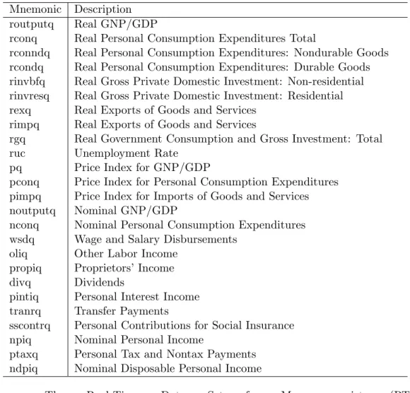
We consider 25 US macro variables which are subject to data revisions. The variables are described in table 1. The data vintages are taken from the Real-Time Data Set for Macro-economists (RTDSM) of Croushore and Stark (2001). Our …rst ‘vintage-origin’is 1996:Q2, and the last is 2011:Q1, so that we have 15 years of quarterly forecast origins. However, the 1999:Q4 and 2009:Q3 vintages contain missing values for many series and these forecast origins are ex-cluded. In order to estimate the models by EOS, we require that each data vintage provides a long enough history of past observations. We use a rolling-window forecasting scheme, where for the …rst vintage origin of 1996:Q2, we use data from 1984 onwards. However, for RTV, we need data vintages going back to 1984 to have data over the same historical period. That is, we require an additional 12 years of data-vintages for RTV estimation. This requirement was satis…ed for the 25 variables forecast in this study.

For all but one of the variables (ruc - the unemployment rate) we model, and evaluate forecasts of, the …rst di¤erence of the natural logarithm. The variable ruc is modelled and forecast untransformed.

To focus on the RTV versus EOS issue, in all cases we use AR(2) models (i.e., two autore-gressive lags), although the number of lags could be selected for each variable at each forecast origin using an information criterion such as BIC. The real-time (EOS) forecasting performance of the AR models (estimated by EOS) has been shown to be improved by discarding the pre-Great Moderation data (Clements (2015)), which is the reason we set the initial start point of the estimation period to 1984. In the …rst instance we use …rst-release actual values. The analysis in section 5 suggests that the distortionary e¤ects of EOS estimation will be relatively muted for forecasting revised data, so we begin with forecasting …rst-release values where we expect the problems with EOS to be clearest. So the actual values are taken from the vintage available one quarter after the target quarter. To evaluate the forecast of 1996:Q2, from the …rst vintage origin of 1996:Q2, for example, we take the observation from the 1996:Q3 data vintage.

standard errors for RTV and EOS estimation; t-statistics of the null that revisions are news;

t-statistics of the null that revisions are noise; and the actual coverage rates of one-step ahead BJ intervals. The tests for news and noise are based on the revisions between the …rst-estimates

y_tt+1, and the data available some three and a half years later y_tt+15, which includes the three rounds of annual regular revisions. We test for news and noise revisions using, respectively:

yt_t+1 yt_t+15= + _ney_tt+1+!t

and:

y_tt+1 y_tt+15= + _noyt_t+15+!t:

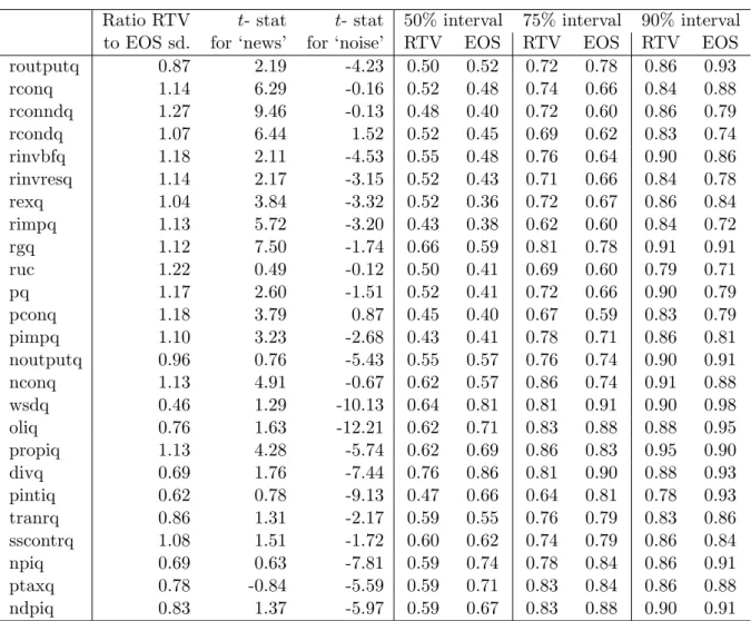
We …nd that 9 of the 25 variables have data revisions which are news, in that we do not reject _ne= 0, but we do reject _no = 0, at conventional levels. For all of these variables the in-sample standard deviation estimated by EOS exceeds the RTV estimate. For the 7 variables for which we do not reject _no = 0 but do reject _ne = 0, implying noise revisions, we …nd the reverse - the EOS standard deviation is smaller than the RTV estimate. Hence for the 16 variables which can be categorized as news or noise, the relative magnitudes of the in-sample standard deviations are as expected given the analysis in section 4. The remaining variables cannot be characterized as purely news or noise, so it is not clear what one would expect to …nd. Aruoba (2008) and Corradi, Fernandez and Swanson (2009) provide recent extensions to testing for the properties of data revisions, but for our purpose of providing a broad classi…cation of each series as being subject to news or noise revisions the standard approach su¢ ces.

In terms of out-of-sample performance, for around 80% of the variables the RTV intervals are more accurate than the EOS intervals, in the sense that the actual coverage rates are closer to the nominal rates. The actual coverage rates are shown for each variable for the RTV and EOS intervals in table 2, but summarizing across all variables, we …nd that the coverage rates of RTV intervals are closer to the nominal for 20, 21 and 18 variables for the50%,75%and90%nominal intervals, respectively. Furthermore, our analysis suggests EOS-interval coverage should exceed that of RTV intervals for variables with news revisions, with the opposite holding for noise revisions. Of the 9 variables categorized as having news revisions, EOS-interval coverage is greater for either all, or all but one, of these variables (depending on the nominal interval size).

Of the 7 variables with noise revisions, the RTV coverage rate is greater for all 7 variables for the50% and75% intervals (and for all but one for the 90% intervals).

As a robustness check, we calculated the statistics reported in table 2 for models with an autoregressive order of one, and found the results were qualitatively unchanged (not reported to save space).

We then supposed the goal of the analysis was to forecast the revised data, either the third estimate, or the fully-revised data (taken to be the value in the 2012:Q3 vintage). We compared the accuracy of intervals based on adapted RTV estimation (with n = 3 in (17), so optimal in population for the third estimate) against intervals based on EOS estimation, for the 25 variables in our study, and using the same setup as for forecasting the …rst-release data. We found that the adapted RTV interval coverage rates were closer to the nominal rates than the EOS intervals for 18, 22 and 16 variables, for the 50%, 75% and 90% coverage-rate intervals, respectively. Hence RTV based on (17) works reasonably well in terms of estimating the uncertainty surrounding the third estimates. For forecasting the fully-revised there was little to choose between RTV (with n= 3) and EOS, with the RTV intervals now being more accurate for 14, 12 and 11 of the variables. In principle n should be set to include the three rounds of annual revisions embodied in the …nal data (so n = 14, say), but this would have meant omitting the last 3 and a half years of quarterly data from the estimation sample at each forecast origin.

RTV estimation is expected to generate more accurate BJ-intervals than EOS because the RTV-estimate of the in-sample standard deviation more accurately re‡ects the out-of-sample uncertainty. Table 2 is designed to show the relationship between the in-sample standard deviations, and the average interval coverage rates. However, obtaining the correct coverage ‘on average’ is a minimal requirement of a sequence of prediction intervals. To see this, let

Ltjt 1(p) and Utjt 1(p) denote the lower and upper limits of a1-step ahead prediction interval

with nominal coverage p, and let It= 1 denote a ‘hit’, de…ned as:

It= 8 < : 1 ifyt2 Ltjt 1(p); Utjt 1(p) ; 0 otherwise (20) for a sequence of forecasts ( L_{tjt 1}(p); U_{tjt 1}(p) ) and realizations (_fytg),t= 1;2; : : : ; N.

Cor-rect unconditional coverage holds when E(It) = p, assessed by whether the sample mean

1

N

PN

t=1It is close top. A more stringent criterion is that the occurrences of1’s and 0’s are

un-predictable - for a given information set_It(whereIt=fIt; It 1;: : :gat a minimum) we require

E(ItjIt 1) =p. When It=fIt; It 1;: : :g, this is equivalent to saying thatfItgis iid Bernoulli

with parameter p. This is a joint test, and Christo¤ersen (1998) presents simple likelihood-based tests of the component parts: correct unconditional coverage (E(It) =p); independence

(against a …rst-order Markov chain structure for _fItg); as well as of the joint hypothesis of

correct conditional coverage. The test for independence will have power to detect (unmodelled) changes in the volatility (because hits will tend to be clustered during the relatively low volatil-ity periods) as well as dynamic mis-speci…cation of the model generating the forecasts. For example, prediction intervals generated by an AR(1)(say), when the data generating process is an AR(2)with gaussian disturbances, will have correct unconditional coverage but not correct conditional coverage. Corradi and Swanson (2006) provide a related discussion in the context of density forecasting.

Table 3 reports the p-values for the tests of correct unconditional coverage (UC), indepen-dence (IND) and conditional coverage (CC) for each variable, for intervals of three nominal sizes (50%, 75% and 90%). The table assumes the goal is to predict the …rst-release values. The penultimate row of the table reports the number of variables for which the null of the corresponding test is rejected (when the test is conducted at the 5% level). The EOS intervals are rejected for more variables than the RTV intervals, and the rejections are mainly of correct unconditional coverage (or ‘bias’), rather than of the test for independence. This indicates that many of the di¤erences between the nominal and actual coverage rates recorded in table 2 for the EOS intervals are statistically signi…cant. When we used adapted-RTV to predict the third-estimates, there was little to choose between RTV and EOS in terms of rejection rates across the set of 25 variables (see last row of table).

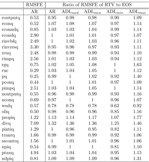
Interval coverage rates may also di¤er because the interval is located about an inaccurate point forecast, and not just because of the scale of the predictive distribution underlying the interval. However, not withstanding the superiority of RTV-estimation in principle for …rst-moment prediction (see Koenig et al.(2003) and Clements and Galvão (2013b)), for our setup we …nd little to choose between the two for the majority of variables, when the point forecasts

of the …rst-release values are evaluated by RMSE: see table 4.

Table 4 shows that RTV improves accuracy by 5% on RMSE for forecasting output growth. But with one or two exceptions, this is at the top end of the gains to RTV, and a number of the entries exceed one, suggesting EOS is more accurate for those variables. This suggests that the RTV-intervals chie‡y bene…t from more accurate estimates of scale rather than location. The general point is that RTV estimation in practical forecasting may matter more for second-moment type forecasts (such as prediction intervals) than for point forecasting.

This last point is supported by the results in table 4 for bivariate ADL (autoregressive-distributed lag) models, where again the aim is to predict the …rst release. For each of the 25 variables we generate EOS and RTV point forecasts for the 24 possible bivariate ADL models, where we include 2 lags of the dependent variable, and of the explanatory variable. This allow us to assess the relative point forecasting performance of RTV compared to EOS for models with explanatory variables which are subject to revision. The results for the ADL models are no more favourable for RTV than the results for AR models. We present the median, mean, minimum and maximum of the ratios across the 24 ADL models for each variable. There is an ADL model (i.e., an explanatory variable) for which RTV is 10% more accurate than EOS for forecasting output growth. But equally there is a variable for which EOS is 9% more accurate for forecasting output growth, and this pattern holds across the majority of variables.

In summary, the empirical estimates of coverage rates are generally in line with the analysis in section 4, and the value of RTV is largely attributable to more accurate estimates of the scale of the predictive distribution, rather than the location (that is, than of the point prediction).

7

Simulation study

We established in section 4 that BJ intervals based on RTV-estimation would be correctly-sized in the presence of data revisions, and that intervals based on EOS-estimation of the model would likely have a coverage in excess of the nominal when data revisions are news, but less than the nominal when data revisions are noise. These statements hold ‘in population’, that is, when we ignore parameter estimation uncertainty, and when the aim is to predict the …rst-release values. Even in the absence of data revisions, it is well known that BJ-intervals can

be adversely a¤ected by parameter estimation uncertainty when the sample size is small. In addition, there will be uncertainty about the model order. Having to select appropriate model orders may a¤ect the relative merits of RTV and EOS. Model selection issues are especially pertinent in our context because the optimal model order for RTV-estimation may di¤er from that using EOS-estimation. To illustrate with a simple case, consider the example in section 4, where the true values follow a zero-mean AR(1)and there is a single noise revision. Hence the data generating process is given by:

yt= yt 1+ t (21)

and the estimates of ytare given by:

y_tt+1 = yt+"t

y_tt+n = yt

(22)

forn= 2;3; : : :. Let the population …rst-order RTV-regression be:

yt_t+1= yt_{t 1}+et;RT V: (23)

where from (15) we know that ₆= when E "2_{t 6}= 0 (i.e., ₆= when there are noise revisions). Substituting for yt_t+1 and yt_{t 1} from (22) into (23) yields et;RT V = yt yt 1 + "t "t 1. Then it follows immediately that the …rst-order model is dynamically-mis-speci…ed

because the second ‘lag’y_tt ₂ (here equal toyt 2) is correlated with the error termet;RT V:

Cov(et;RT V; yt 2) =Cov(yt yt 1; yt 2) +Cov("t "t 1; yt 2):

The second covariance on the RHS is zero, and the …rst is only zero when = , in which case

yt yt 1 = t.

For these reasons we investigate the small-sample properties of the procedures by simula-tion, allowing that the appropriate model orders need to be selected by an information criterion, such as BIC. Of interest is whether RTV-estimation provides accurate intervals in these cir-cumstances.

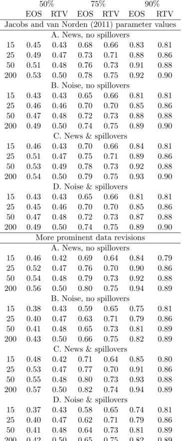
Simulating data with revisions requires a complete speci…cation of the data revisions process. This requires giving values to a relatively large number of parameters, and the concomitant concern that the results of the simulation study may be speci…c to the range of values considered. In order to obtain sensible values for the data generating process, we use the model estimated by Jacobs and van Norden (2011) for US real output growth as our base case. They allow for data revisions to be news or noise, with and without ‘spillovers’. We also experiment with a variant in which the standard deviation of the underlying shock is divided by 4, but the standard deviations of the news and noise disturbances (and all the other parameters) are left unaltered, to gauge the impact of data revisions being more prominent (than they are for real output, as estimated by Jacobs and van Norden (2011)). To save space, we do not repeat the details of their model, except to note that there are four vintage estimates of each time period, and the …nal is not assumed to reveal the truth (i.e., yt_t+4 ₆=yt). The estimated parameter values

that we use are taken from their Table 1 (p.107). We simulate 25;000 replications of length

T+ 1, after discarding initial observations to remove any dependence on initial conditions, and on each sample we estimate the AR model by EOS and RTV on the …rst T observations, and calculate a BJ prediction interval for the …rst estimate of theT+ 1observation (i.e., yT_T+2₊₁).

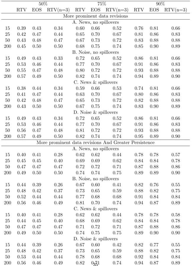
The results are recorded in table 5. For the Jacobs and van Norden (2011) data generating process (top half of table) the RTV intervals are under-sized at small T but approximately correctly-sized at larger T. The coverage rates are similar (for a given T) whether revisions are news of noise, and irrespective of whether there are spillovers: RTV-intervals are largely immune to the e¤ects of data revisions. This is underlined by comparing these estimated coverage rates with those when there are no revisions (recorded at the foot of the table): the two sets are virtually identical. It is well known in the literature that neglecting the uncertainty inherent in the estimated model parameters will lead to under-sized intervals, and this e¤ect is obviously more pronounced at small T. By contrast, EOS-estimation is not a reliable method of generating prediction intervals, giving rise to intervals which are under-sized or over-sized, depending on T, when revisions are news. When revisions are more prominent (second half of table), the performance of the EOS intervals worsens, and the EOS intervals are clearly under-sized when there is noise. Whereas the performance of the RTV intervals is virtually una¤ected. There is little appreciable e¤ect from allowing spillovers.

Table 6 presents Monte Carlo estimates of coverage rates for forecasting the revised data (here, the fourth estimate). We report results for experiments matching the second half of table 5 (i.e., the more prominent revisions), as well as when the autoregressive parameters are larger (at 0:90 and 0:05), in the second half of the table. The table gives the results of using RTV, EOS and adapted RTV. As expected, the costs to using EOS in terms of biased coverage rates are reduced relative to forecasting early-release data. In the top half of the table, for example, the large-sample coverage rates are correct, as are those of adapted RTV (as expected). The intervals for RTV tuned to …rst-release forecasting are not correct, even in large samples. The small-sample performance of the adapted RTV intervals is adversely a¤ected by the loss of observations. The second half of the table indicates that when the process is highly persistent the EOS intervals may be incorrectly-sized even in large samples, whereas the adapted RTV estimates remain correctly-sized .

Table 7 records the rejection frequencies of the tests for unconditional coverage, indepen-dence and conditional coverages, for forecasting the …rst-release data. Although we include the test for independence (and correct conditional coverage), in the absence of unmodelled time-varying heteroscedasticity we would not expect this test to deviate much from its nominal size, and that transpires to be the case. The rejection frequencies are based on generated sequences of 100 prediction intervals and actuals. The initial sample size is recorded in the table, and the model is re-estimated (by EOS or RTV) on an expanding window of data prior to calculating the interval. For the resulting vector of hits and misses, we calculate the three tests. The table records the rejection frequencies across 10,000 replications of this procedure. For the RTV intervals, there are some minor size distortions at the smaller sample sizes, but otherwise the tests are correctly sized, while the EOS intervals are clearly inadequate, and this is ‡agged by the tests of coverage. For the selected Monte Carlo data-generation process parameter values, the rejections are greater for noise revisions, and for the 75% and 90% nominal intervals are in excess of 50%. We conclude that prediction intervals from RTV-estimation with BIC model-order speci…cation generates intervals with desirable properties, whilst the traditional approach (EOS-estimation) does not.

8

Conclusions

We have shown that assessments of future macroeconomic uncertainty based on the in-sample …t of a model are likely to be misleading when the variable being modelled is subject to revision. This is particularly true when the aim is to predict an early-vintage estimate of a future obser-vation. Then the data on which the model is estimated will be for the most part fully-revised or mature data, whereas the out-of-sample value is a …rst-release or only lightly-revised data point. In the context of …rst-moment prediction Kishor and Koenig (2012) referred to esti-mating the model on fully-revised data, and conditioning the forecast on only lightly-revised data, as mixing ‘apples and oranges’. In the context of second-moment prediction the mismatch results instead from supposing the goodness of …t of the model on the fully-revised data (i.e., the in-sample period) is an accurate representation of the out-of-sample …t.

For forecasting revised or mature values of future observations we show that these concerns are alleviated.

We have shown that a simple solution is to use real-time-vintage (RTV) data. This was pro-posed by Koeniget al.(2003) in the context of …rst-moment prediction. Based on the evidence for the 25 macro variables we consider in this paper, RTV-estimation is more bene…cial for second-moment forecasting. Its validity in population (abstracting from parameter estimation uncertainty) is easily established. Its good forecast performance has been demonstrated, and is supported by a simulation study.

We have considered autoregressive models in this paper, but the logic of the arguments suggests that the …ndings carry over immediately to models with explanatory variables, so the problems with using EOS, and the advantages of RTV, are potentially more generally applica-ble. For example, there has been much interest in measuring macro-uncertainty in the recent literature, driven in large part by the belief that time-varying uncertainty may play an impor-tant role in business cycle ‡uctuations (see, e.g., Bachmann, Elstner and Sims (2013)). Some of the approaches to measuring macro-uncertainty use ‘data-rich’modelling environments, and are pseudo real-time, perhaps because of the di¢ culties of collecting and managing di¤erent data vintages at each point in time. Two recent closely-related contributions are Jurado, Lud-vigson and Ng (2015) and Henzel and Rengel (2013). As pseudo-real time exercises, the e¤ects of data revisions are side-stepped. However, the measures of macro uncertainty are derived

from the individual variables’forecast errors, rather than the in-sample …ts of the models, and so would be immune to the distorting e¤ects described in this paper if similar exercises were carried out in real time. For example, Jurado et al.(2015) calculate forecast errors for each of a large number of variables using a factor model, and then …t a stochastic volatility model to the forecast errors to obtain individual-variable volatility forecasts, which are then aggregated. Other approaches which use instead the in-sample …t of the model - as in the standard approach to calculating prediction intervals illustrated in this paper - are likely to be misleading in the presence of data revisions.

References

Aruoba, S. B. (2008). Data revisions are not well-behaved. Journal of Money, Credit and Banking,40, 319–340.

Bachmann, R., Elstner, S., and Sims, E. R. (2013). Uncertainty and economic activity: Evidence from Business Survey Data. American Economic Journal: Macroeconomics, 5(2), 217– 249.

Box, G. E. P., and Jenkins, G. M. (1970). Time Series Analysis, Forecasting and Control. San Francisco: Holden-Day.

Christo¤ersen, P. F. (1998). Evaluating interval forecasts. International Economic Review,39, 841–862.

Clements, M. P. (2015). Real-time factor model forecasting and the e¤ects of instability. Com-putational Statistics and Data Analysis. doi:10.1016/j.csda.2015.01.011, Forthcoming. Clements, M. P., and Galvão, A. B. (2012). Improving real-time estimates of output gaps and

in‡ation trends with multiple-vintage VAR models. Journal of Business and & Economic Statistics,30(4), 554–562. DOI: 10.1080/07350015.2012/707588.

Clements, M. P., and Galvão, A. B. (2013a). Forecasting with vector autoregressive models of data vintages: US output growth and in‡ation. International Journal of Forecasting,

29(4), 698 –714. DOI: 10.1016/j.ijforecast.2011.09.003.

Clements, M. P., and Galvão, A. B. (2013b). Real-time forecasting of in‡ation and output growth with autoregressive models in the presence of data revisions. Journal of Applied Econometrics,28(3), 458–477. DOI: 10.1002/jae.2274.

Corradi, V., Fernandez, A., and Swanson, N. R. (2009). Information in the revision process of real-time datasets. Journal of Business and Economic Statistics,27, 455–467.

Corradi, V., and Swanson, N. R. (2006). Bootstrap conditional distribution tests in the presence of dynamic misspeci…cation. Journal of Econometrics,133(2), 779–806.

Croushore, D. (2011a). Forecasting with real-time data vintages, chapter 9. In Clements, M. P., and Hendry, D. F. (eds.), The Oxford Handbook of Economic Forecasting, pp. 247–267: Oxford University Press.

Croushore, D. (2011b). Frontiers of real-time data analysis. Journal of Economic Literature,

49, 72–100.

Croushore, D., and Stark, T. (2001). A real-time data set for macroeconomists. Journal of Econometrics,105(1), 111–130.

Cunningham, A., Eklund, J., Je¤ery, C., Kapetanios, G., and Labhard, V. (2009). A state space approach to extracting the signal from uncertain data. Journal of Business & Economic Statistics,30, 173–180. doi:10.1198/jbes.2009.08171.

Faust, J., Rogers, J. H., and Wright, J. H. (2003). Exchange rate forecasting: The errors we’ve really made. Journal of International Economic Review,60, 35–39.

Garratt, A., Lee, K., Mise, E., and Shields, K. (2008). Real time representations of the output gap. Review of Economics and Statistics,90, 792–804.

Garratt, A., Lee, K., Mise, E., and Shields, K. (2009). Real time representations of the UK output gap in the presence of model uncertainty. International Journal of Forecasting,

25, 81–102.

Harvey, A. C., McKenzie, C. R., Blake, D. P. C., and Desai, M. J. (1983). Irregular data revisions. In Zellner, A. (ed.),Applied Time Series Analysis of Economic Data, pp. 329– 347: US Department of Commerce, Washington D.C., Economic Research Report ER-5. Henzel, S., and Rengel, M. (2013). Dimensions of macroeconomic uncertainty: A common factor analysis. Ifo working paper series, Ifo Institute for Economic Research at the University of Munich.

Howrey, E. P. (1984). Data revisions, reconstruction and prediction: an application to inventory investment. The Review of Economics and Statistics,66, 386–393.

Jacobs, J. P. A. M., and van Norden, S. (2011). Modeling data revisions: Measurement error and dynamics of ‘true’values. Journal of Econometrics,161, 101–109.

Jurado, K., Ludvigson, S. C., and Ng, S. (2015). Measuring Uncertainty. American Economic Review,105(3), 1177–1216.

Kishor, N. K., and Koenig, E. F. (2012). VAR estimation and forecasting when data are subject to revision. Journal of Business and Economic Statistics,30(2), 181–190.

forecasting. The Review of Economics and Statistics,85(3), 618–628.

Landefeld, J. S., Seskin, E. P., and Fraumeni, B. M. (2008). Taking the pulse of the economy.

Journal of Economic Perspectives,22, 193–216.

Mankiw, N. G., and Shapiro, M. D. (1986). News or noise: An analysis of GNP revisions.Survey of Current Business (May 1986), US Department of Commerce, Bureau of Economic Analysis, 20–25.

Orphanides, A. (2001). Monetary policy rules based on real-time data. American Economic Review,91(4), 964–985.

Orphanides, A., and van Norden, S. (2005). The reliability of in‡ation forecasts based on output gaps in real time. Journal of Money, Credit and Banking,37, 583–601.

Patterson, K. D. (1995). An integrated model of the data measurement and data generation processes with an application to consumers’expenditure. Economic Journal,105, 54–76. Patterson, K. D. (2003). Exploiting information in vintages of time-series data. International

Journal of Forecasting,19, 177–197.

Robertson, J. C., and Tallman, E. W. (1998). Data vintages and measuring forecast model performance. Federal Reserve Bank of Atlanta Economic Review, Fourth Quarter, 4–20. Thombs, L. A., and Schucany, W. R. (1990). Bootstrap prediction intervals for autoregression.

Acknowledgments

The helpful comments and suggestions of two referees of this journal are gratefully acknowl-edged.

Table 1: Data Description Mnemonic Description

routputq Real GNP/GDP

rconq Real Personal Consumption Expenditures Total

rconndq Real Personal Consumption Expenditures: Nondurable Goods rcondq Real Personal Consumption Expenditures: Durable Goods rinvbfq Real Gross Private Domestic Investment: Non-residential rinvresq Real Gross Private Domestic Investment: Residential rexq Real Exports of Goods and Services

rimpq Real Exports of Goods and Services

rgq Real Government Consumption and Gross Investment: Total ruc Unemployment Rate

pq Price Index for GNP/GDP

pconq Price Index for Personal Consumption Expenditures pimpq Price Index for Imports of Goods and Services noutputq Nominal GNP/GDP

nconq Nominal Personal Consumption Expenditures wsdq Wage and Salary Disbursements

oliq Other Labor Income propiq Proprietors’Income divq Dividends

pintiq Personal Interest Income tranrq Transfer Payments

sscontrq Personal Contributions for Social Insurance npiq Nominal Personal Income

ptaxq Personal Tax and Nontax Payments ndpiq Nominal Disposable Personal Income

Source: The Real-Time Data Set for Macroeconomists (RTDSM), http://www.philadelphiafed.org/research-and-data/real-time-center/real-time-data/, see Croushore and Stark (2001).

Table 2: RTV and EOS Box-Jenkins Prediction Intervals Coverage Rates for RTV and EOS Ratio RTV t- stat t- stat 50%interval 75%interval 90%interval to EOS sd. for ‘news’ for ‘noise’ RTV EOS RTV EOS RTV EOS routputq 0.87 2.19 -4.23 0.50 0.52 0.72 0.78 0.86 0.93 rconq 1.14 6.29 -0.16 0.52 0.48 0.74 0.66 0.84 0.88 rconndq 1.27 9.46 -0.13 0.48 0.40 0.72 0.60 0.86 0.79 rcondq 1.07 6.44 1.52 0.52 0.45 0.69 0.62 0.83 0.74 rinvbfq 1.18 2.11 -4.53 0.55 0.48 0.76 0.64 0.90 0.86 rinvresq 1.14 2.17 -3.15 0.52 0.43 0.71 0.66 0.84 0.78 rexq 1.04 3.84 -3.32 0.52 0.36 0.72 0.67 0.86 0.84 rimpq 1.13 5.72 -3.20 0.43 0.38 0.62 0.60 0.84 0.72 rgq 1.12 7.50 -1.74 0.66 0.59 0.81 0.78 0.91 0.91 ruc 1.22 0.49 -0.12 0.50 0.41 0.69 0.60 0.79 0.71 pq 1.17 2.60 -1.51 0.52 0.41 0.72 0.66 0.90 0.79 pconq 1.18 3.79 0.87 0.45 0.40 0.67 0.59 0.83 0.79 pimpq 1.10 3.23 -2.68 0.43 0.41 0.78 0.71 0.86 0.81 noutputq 0.96 0.76 -5.43 0.55 0.57 0.76 0.74 0.90 0.91 nconq 1.13 4.91 -0.67 0.62 0.57 0.86 0.74 0.91 0.88 wsdq 0.46 1.29 -10.13 0.64 0.81 0.81 0.91 0.90 0.98 oliq 0.76 1.63 -12.21 0.62 0.71 0.83 0.88 0.88 0.95 propiq 1.13 4.28 -5.74 0.62 0.69 0.86 0.83 0.95 0.90 divq 0.69 1.76 -7.44 0.76 0.86 0.81 0.90 0.88 0.93 pintiq 0.62 0.78 -9.13 0.47 0.66 0.64 0.81 0.78 0.93 tranrq 0.86 1.31 -2.17 0.59 0.55 0.76 0.79 0.83 0.86 sscontrq 1.08 1.51 -1.72 0.60 0.62 0.74 0.79 0.86 0.84 npiq 0.69 0.63 -7.81 0.59 0.74 0.78 0.84 0.86 0.91 ptaxq 0.78 -0.84 -5.59 0.59 0.71 0.83 0.84 0.86 0.88 ndpiq 0.83 1.37 -5.97 0.59 0.67 0.83 0.88 0.90 0.91 The second column reports the ratio of the estimated in-sample standard errors for RTV to EOS. (The EOS standard deviation is the average of the standard deviations calculated for each of the 58 rolling window estimation samples. The RTV sd. is calculated similarly). The third and fourth columns record thet-statistics for tests that the 1st-estimate to 15th-estimate revisions are news and noise, respectively. These tests are run once for each variable and relate to observation periods 1970:Q2 to 2007:Q2. The remaining columns record coverage rates for nominal coverages of 50%,75%and 90%.

For both AR and EOS the model is an AR(2), estimated on forecasts (vintage) origins 1996:Q2 to 2011:Q1, using a rolling window of observations (and an initial window estimated on post 1984 observations). We omit the 1999:Q4 and 2009:Q3 vintages which contain missing values for many of the series.

For the Bureau of National Accounts variables the RTDSM contains missing values for the 1996:Q1 estimates of 1995:Q4. These do not a¤ect the EOS forecasts, because the …rst forecast origin is 1996:Q2, but these missing values do a¤ect all RTV forecasts. We have simply set the values for 1995:Q4 to the 1995:Q3 values in the same (1996:Q1) vintage.

T able 3: F ormal tests of R TV and EOS prediction in terv als Nominal Co v erage 50% Nominal Co v erage 75% Nominal Co v erage 90% R TV EOS R TV EOS R TV EOS UC IND CC UC IND CC UC IND CC UC IND CC UC IND CC UC IND CC routputq 1 0.90 0.99 0.79 0.89 0.96 0.65 0.24 0.45 0.65 0.14 0.30 0.36 0.07 0.12 0.41 0.23 0.35 rconq 0.79 0.69 0.89 0.79 0.67 0.88 0.88 0.51 0.80 0.11 0.23 0.13 0.19 0.15 0.15 0.61 0.21 0.40 rconndq 0.79 0.67 0.88 0.11 0.40 0.20 0.65 0.08 0.20 0.01 0.69 0.05 0.36 0.89 0.65 0.02 0.71 0.05 rcondq 0.79 0.70 0.89 0.43 0.39 0.51 0.30 0.67 0.53 0.03 0.16 0.04 0.09 0.82 0.24 0 0.97 0 rin vbfq 0.43 0.65 0.66 0.79 0.52 0.79 0.88 0.08 0.21 0.06 0.20 0.07 0.93 0.01 0.03 0.36 0.37 0.44 rin vresq 0.79 0.01 0.04 0.29 0.18 0.23 0.46 0.07 0.15 0.11 0 0 0.19 0.15 0.15 0.01 0.14 0.01 rexq 0.79 0.35 0.63 0.03 0.57 0.09 0.65 0.11 0.25 0.19 0.12 0.12 0.36 0.37 0.44 0.19 0.15 0.15 rimp q 0.29 0.11 0.16 0.06 0.01 0.01 0.03 0.95 0.09 0.01 0.63 0.04 0.19 0.15 0.15 0 0.89 0 rgq 0.02 0.32 0.04 0.19 0.69 0.39 0.27 0.95 0.55 0.65 0.67 0.82 0.72 0.31 0.56 0.72 0.23 0.46 ruc 1 0.23 0.49 0.19 0.30 0.25 0.30 0.07 0.11 0.01 0.05 0.01 0.02 0.04 0.01 0 0.11 0 p q 0.79 0.51 0.78 0.19 0.07 0.08 0.65 0.74 0.86 0.11 0.23 0.13 0.93 0.63 0.88 0.02 0.71 0.05 p conq 0.43 0.39 0.51 0.11 0.53 0.24 0.19 0.12 0.12 0.01 0.63 0.02 0.09 0.06 0.04 0.02 0.06 0.01 pimp q 0.29 0.02 0.04 0.19 0.21 0.19 0.65 0.11 0.25 0.46 0.49 0.60 0.36 0.11 0.18 0.04 0.02 0.01 noutputq 0.43 0.20 0.32 0.29 0.98 0.57 0.88 0.56 0.83 0.88 0.17 0.39 0.93 0.10 0.26 0.72 0.41 0.67 nconq 0.06 0.78 0.17 0.29 0.60 0.50 0.04 0.37 0.07 0.88 0.48 0.77 0.72 0.41 0.67 0.61 0.87 0.87 wsdq 0.03 0.72 0.10 0 0 0 0.27 0.09 0.13 0 0.04 0 0.93 0.06 0.18 0.01 0.85 0.04 oliq 0.06 0.95 0.18 0 0.49 0 0.16 0.56 0.31 0.01 0.16 0.02 0.61 0.74 0.83 0.18 0.56 0.35 propiq 0.06 0.16 0.07 0 0.70 0.01 0.04 0.89 0.11 0.16 0.82 0.36 0.18 0.11 0.11 0.93 0.63 0.88 divq 0 0 0 0 0 0 0.27 0 0 0 0 0 0.61 0 0.01 0.41 0.01 0.03 pin tiq 0.60 0.05 0.12 0.02 0 0 0.06 0.01 0 0.27 0.47 0.42 0.01 0 0 0.41 0.23 0.35 tranrq 0.19 0.21 0.19 0.43 0.75 0.70 0.88 0.69 0.91 0.44 0.26 0.39 0.09 0.28 0.13 0.36 0.37 0.44 sscon trq 0.11 0 0 0.06 0.03 0.02 0.88 0.37 0.66 0.44 0.19 0.31 0.36 0.04 0.08 0.19 0.10 0.11 npiq 0.19 0.21 0.19 0 0 0 0.65 0 0.01 0.08 0.10 0.06 0.36 0.28 0.37 0.72 0.41 0.67 ptaxq 0.19 0.13 0.14 0 0 0 0.16 0.21 0.16 0.08 0 0 0.36 0.07 0.12 0.61 0.21 0.40 ndpiq 0.19 0.30 0.25 0.01 0.32 0.02 0.16 0.82 0.36 0.01 0.02 0 0.93 0.10 0.26 0.72 0.41 0.67 Rejs (1st estimate) 3 5 5 9 7 10 3 3 3 9 5 11 2 5 5 9 2 8 Rejs (3rd estimate) 3 8 7 9 9 9 4 8 9 7 5 10 6 8 8 7 6 9 The eleme n ts of the table (bar those in the b ottom ro w) are p -v alues of the the n ull of correct unconditional co v erage (UC), indep endence (IND) and conditional co v erage (C C) when the aim is to preduct … rst-release actuals. The p en ultimate ro w elemen ts are the n um b ers of v ariables for whic h the p -v alues in the corresp onding column s are less than 0 : 05 . The … nal ro w presen ts the n um b er of v ariables for whic h the corresp onding test rejec ts when EOS and adapted R TV (with n = 3 ) are u sed to predict the third estimates.

Table 4: RTV and EOS forecasts with AR models and ADL RMSFE Ratio of RMSFE of RTV to EOS

AR AR ADLmed ADLmea ADLmin ADLmax

routputq 0.53 0.95 0.98 0.98 0.90 1.09 rconq 0.52 1.07 1.08 1.07 0.97 1.14 rconndq 0.85 1.03 1.03 1.04 0.99 1.14 rcondq 2.90 1 1.01 1.01 0.97 1.07 rinvbfq 2.49 1 1.02 1.03 0.96 1.11 rinvresq 3.30 0.95 0.96 0.97 0.93 1.11 rexq 2.48 0.98 0.98 0.99 0.94 1.10 rimpq 2.56 1.01 1.03 1.03 0.94 1.12 rgq 0.75 1.02 1.05 1.08 1 1.63 ruc 0.29 1.03 1.04 1.05 1 1.12 pq 0.25 0.99 1 1.02 0.92 1.40 pconq 0.44 1 1 1.01 0.97 1.09 pimpq 2.51 1.03 1.04 1.05 1 1.14 noutputq 0.55 0.96 0.98 0.99 0.93 1.16 nconq 0.69 0.97 1 1 0.96 1.07 wsdq 0.57 0.78 0.78 0.78 0.62 0.92 oliq 0.50 0.98 0.96 0.96 0.85 1.16 propiq 1.22 1.13 1.14 1.17 1.07 1.77 divq 7.09 1.32 1.36 1.36 1.25 1.46 pintiq 1.29 1 0.96 0.95 0.82 1.11 tranrq 1.66 0.98 0.98 0.99 0.92 1.06 sscontrq 1.56 1 1.01 1.01 0.96 1.06 npiq 0.54 0.99 1 1 0.81 1.10 ptaxq 4.94 1.03 1.04 1.04 0.95 1.15 ndpiq 0.81 1.09 1.09 1.09 0.96 1.31

Notes. The table reports the RMSEs for a rolling forecasting scheme, with initial window beginning in 1984:Q1. Out-of-sample forecast period is 1996:Q2 to 2011:Q1. The actual values used to calculate forecast errors are …rst-release values.