Improved Guidelines for Recalibration of Predictive Models over Time Based on Model Uncertainty

(1)

IMPROVED GUIDELINES FOR RECALIBRATION OF PREDICTIVE MODELS OVER TIME BASED ON MODEL UNCERTAINTY

A Thesis by

BHARADWAJ BOMMANAYAKANAHALLI

Submitted to the Office of Graduate and Professional Studies of Texas A&M University

in partial fulfillment of the requirements for the degree of MASTER OF SCIENCE Chair of Committee, Committee Members, Head of Department, Dominique Lord Yunlong Zhang Daren B.H. Cline Robin Autenrieth May 2018

Major Subject: Civil Engineering

(2)

ii

ABSTRACT

The Highway Safety Manual (HSM) summarizes the safety performance functions (SPFs) of various facility types. The primary use of SPFs is to estimate the safety performance (i.e., the number of crashes by severity level) of different facilities based on geometric and traffic variables. The SPFs were developed using the negative binomial (NB) regression model based on crash data obtained from a selected number of states and cities in the United States and Canada. Applied directly to the local jurisdictions, SPFs may yield biased or incorrect results. Therefore, calibration of the SPFs or predictive models is an important step before applying them to local jurisdictions. Moreover, it is also necessary to recalibrate SPFs over time to account for variations in factors that cannot be accounted for directly in SPFs, such as changes in driver behavior, crash-reporting thresholds, etc. The calibration factor (for a specific facility type) is defined as the ratio of the observed number of crashes to the predicted number of crashes. The HSM recommends that SPFs be recalibrated every 2 to 3 years. However, these guidelines are not based on sound research or reliable criteria. The lack of appropriate guidelines can lead to two types of errors: recalibrating of the models when it is not needed, and not recalibrating them when such a need arises.

The aim of this thesis is to develop guidelines regarding when or how often SPFs should be recalibrated. To this end, two methodologies were created related to the variance or

uncertainty associated with the SPFs, and the guidelines were developed using statistical principles. These guidelines are that SPFs should be recalibrated when (i) the total number of crashes that occur in a network of similar types of facilities falls beyond the prediction intervals

(3)

iii

of the predicted or estimated total number of crashes in that same network; or (ii) the calibration factor developed in a specific year is statistically significantly different than 1 (based on

coefficient of variation (CV) of the SPF and the Calibration Factor C).

Both approaches were tested on several intersections and segment datasets from Michigan and Toronto. The results show that both approaches are feasible and could provide safety analysts with better and more reliable guidelines regarding when SPFs should be

recalibrated. However, the methodologies developed in this thesis cannot be applied to the SPFs developed in the HSM since the information needed to evaluate the variance of SPFs is not available in this manual. The results of both the methodologies were compared to the results of a methodology recently proposed in the literature that can be applied to HSM SPFs and uses a fixed threshold value of C-factor error estimate (say 10%). This study indicated that the 10% error is a reasonable value to use for re-calibrating models.

The shortcomings of these methodologies include the need to develop a new SPF (which is time-consuming and work-intensive process) and to collect extensive data every year. When data is available every year, the practitioner might as well estimate a new calibration factor every year instead of needing to know the frequency of recalibration or use an approximate method (C-proxy). Future research in this area should focus on identifying the minimum data requirements for both methodologies proposed in this thesis.

(4)

iv

DEDICATION

(5)

v

ACKNOWLEDGEMENTS

I would like to thank my advisor, Dr. Dominique Lord who came up with this research idea and helped me a lot over the course of the research. I would also like to thank Dr. Yunlong Zhang and Dr. Daren Cline for serving as the members of my thesis committee. Moreover, I would like to thank Mr. Mohammad Ali Shirazi who spent a lot of his time in clarifying my doubts and helped me in the process of understanding the problem statement better.

The Transportation Engineering Graduate Program at Texas A&M has been one of the best experiences in my life. The term papers and design projects I did as part of my coursework improved my critical thinking abilities and reinforced my interest in this specialization. I would like to specially thank Dr. Gene Hawkins and Dr. Mark Burris under whom I took some of the best courses in the transportation program.

I am immensely grateful to Mr. Adam Pike who offered me the position of Graduate Research Assistant in the Signs and Markings program of Texas A&M Transportation Institute. Under his supervision, I worked on several projects related to pavement markings and developed a good understanding of research in that area. The paper that we both wrote “Development of a pavement marking life cycle cost tool” has been selected for publication in the Transportation Research Record (TRR). I also worked as a Graduate Student Worker under Dr. Subasish Das in the Roadway Safety division. Under his supervision I developed skills in crash data reduction and modeling. I received exposure to the various kinds of safety projects during this time.

I am very grateful to my parents for supporting my decision to pursue higher studies in the United States. I also would like to thank almighty God for blessing me with whatever I have in my life today.

(6)

vi

CONTRIBUTORS AND FUNDING SOURCES

Contributors

This work was supported by a thesis committee consisting of Dr. Dominique Lord and Dr. Yunlong Zhang of the Department of Civil Engineering and Dr. Daren Cline of the Department of Statistics.

The Toronto dataset used for analysis in this thesis was provided by Dr. Dominique Lord and the Michigan dataset was provided by Dr. Srinivas Geedipally of the Texas A&M

Transportation Institute. The procedure to evaluate the variance associated with the predictive models (of crashes) has been adopted from the work done by Wood published in 2005 in Accident Analysis and Prevention. The concept proposed by Dr. Ezra Hauer in the NCHRP report HR 20-7(332) published in 2014 was used for evaluating the coefficient of variation of the calibration factor.

All other work completed for the thesis was completed by the student independently. Funding Sources

There are no outside funding contributions to acknowledge related to the research and compilation of this document.

(7)

vii

NOMENCLATURE

AIC Akaike Information Criterion AADT Annual Average Daily Traffic BIC Bayesian Information Criterion

CI Confidence Interval

C-Factor Calibration Factor

CMF Crash Modification Factor CV Coefficient of variation DOT Department of Transportation

HSM Highway Safety Manual

m Safety at a site

MAD Median Absolute Deviance MSPE Mean Square Prediction Error

NB Negative Binomial

PI Prediction Interval

SPF Safety Performance Function

Y Observed number of crashes at a site

(8)

viii

LIST OF FIGURES

Page

Figure 1. Flow chart for the first methodology proposed for recalibration ... 22

Figure 2. Flow chart for the second methodology proposed for recalibration... 25

Figure 3. Illustration of first method for Toronto 4-legged intersections ... 39

Figure 4. Illustration of Shirazi et al. (2017) method for Toronto 4-legged intersections ... 39

Figure 5. Illustration of first method for Michigan 3-legged intersections ... 43

Figure 6. Illustration of Shirazi et al. (2017) method for Michigan 3-legged intersections ... 43

Figure 7. Illustration of first method for Michigan 4-legged intersections ... 47

Figure 8. Illustration of Shirazi et al. (2017) method for Michigan 4-legged intersections ... 47

Figure 9. Illustration of first method for Michigan 2-lane undivided segments ... 51

Figure 10. Illustration of Shirazi et al. (2017) method for Michigan 2-lane undivided segments.51 Figure 11. Illustration of first method for Michigan 4-lane undivided segments ... 55

Figure 12. Illustration of Shirazi et al. (2017) method for Michigan 4-lane undivided segments.55 Figure 13. Illustration of first method for Michigan 4-lane divided segments ... 59

(11)

xi

LIST OF TABLES

Page

Table 1. Summary of the estimated variance and 95% CI/PI for the quantities ... 20

Table 2. Summary statistics of the Toronto 4-legged intersections data ... 27

Table 3. Summary statistics for Michigan 3-legged intersections data ... 28

Table 4. Summary statistics for Michigan 4-legged intersections data ... 29

Table 5. Summary statistics for Michigan 2-lane undivided segments data... 30

Table 6. Summary statistics for Michigan 4-lane undivided segments data... 31

Table 7. Summary statistics for Michigan 4-lane divided segments data... 32

Table 8. Model output for the Toronto 4-legged intersections ... 36

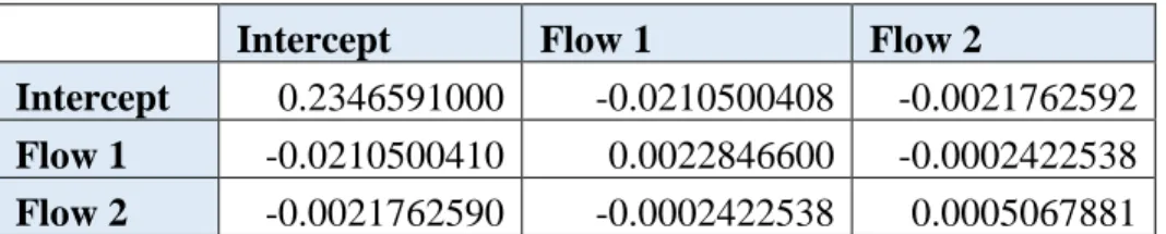
Table 9. Variance-covariance matrix for the Toronto 4-legged intersection model ... 37

Table 10. Summary of the results for Toronto 4-legged intersections based on first methodology and Shirazi et al. (2017) ... 38

Table 11. Model output for the Michigan 3-legged intersections ... 40

Table 12. Variance-covariance matrix for the Michigan 3-legged intersection model ... 40

Table 13. Summary of the results for Michigan 3-legged intersections based on first methodology and Shirazi et al. (2017) ... 42

Table 14. Model output for the Michigan 4-legged intersections ... 44

Table 15. Variance-covariance matrix for the Michigan 4-Legged intersection model ... 44

Table 16. Summary of the results for Michigan 4-legged intersections based on first methodology and Shirazi et al. (2017) ... 46

Table 17. Model output for the Michigan 2-lane undivided segments ... 48

Table 18. Variance-covariance matrix for the Michigan 2-lane undivided segment model ... 48

Table 19. Summary of the results for Michigan 2-lane undivided segments based on first methodology and Shirazi et al. (2017) ... 50

(12)

xii

Page Table 20. Model output for the Michigan 4-lane undivided segments ... 52 Table 21. Variance-covariance matrix for the Michigan 4-lane undivided segment model ... 53 Table 22. Summary of the results for Michigan 4-lane undivided segments based on first

methodology and Shirazi et al. (2017) ... 54 Table 23. Model output for the Michigan 4-lane divided segments ... 56 Table 24. Variance-covariance matrix for the Michigan 4-lane divided segment model ... 56 Table 25. Summary of the results for Michigan 4-lane divided segments based on first

methodology and Shirazi et al. (2017) ... 58 Table 26. Summary of the results for Toronto 4-legged intersections based on second

methodology ... 61 Table 27. Summary of the results for Michigan 3-legged intersections based on second

methodology ... 61 Table 28. Summary of the results for Michigan 4-legged intersections based on second

methodology ... 63 Table 29. Summary of the results for Michigan 2-lane undivided segments based on second

methodology ... 63 Table 30. Summary of the results for Michigan 4-lane undivided segments based on second

methodology ... 65 Table 31. Summary of the results for Michigan 4-lane divided segments based on second

(13)

1

CHAPTER I

INTRODUCTION

This chapter presents the problem statement and objectives of this study. This is followed by an overview of the thesis.

1.1PROBLEM STATEMENT

Traffic safety analysts often examine different alternatives to the design of a roadway or intersection to evaluate the safety associated with each of the designs. Moreover, they are also interested in identifying crash hotspots and the effects of traffic and geometric variables on the number of crashes and their severity. These analysts should be able to predict the frequency and severity of crashes beforehand to estimate the safety effects in the design before the different projects are ranked based on safety or sent into the construction phase. To achieve this, crash prediction models must be developed. There are several challenges associated with developing predictive models. First, analysts need to appropriately identify all the variables (geometric, traffic, human factors, etc.) that could potentially affect the number of crashes on a specific facility. Moreover, in addition to data quality, the sample size of the data should be large enough to develop a reliable model. All these activities require significant time and effort.

The first edition of the Highway Safety Manual (HSM) (AASHTO, 2010) was created to enable different safety analyses to be conducted in a simple manner. The current edition of the HSM summarizes safety performance functions (SPFs) for rural two-lane roads and multilane highways, urban/suburban arterials, freeways, and interchanges. The SPFs in the HSM were developed using a negative binomial (NB) regression model with data collected from a selected number of cities and states in the United States and Canada (Bahar, 2014). The SPFs in the HSM

(14)

2

refer to the safety performance of roadway segments or intersections for the base conditions (note: the base conditions vary by facility type and are described in more detail in the HSM). The base conditions usually refer to the most commonly used highway design and operational

characteristics, such as 12-ft lanes and no-turning lanes at intersections. The effect of variations from the base conditions (like an 11-ft lane) is considered in the SPFs using crash modification factors (CMFs). The value of the CMFs is an indication of the effectiveness of a treatment. A value of CMF greater than 1 indicates an increase in crash frequency due to the treatment, whereas a value less than 1 indicates a decrease.

The SPFs described in the HSM cannot be directly used for a particular jurisdiction since the SPFs do not directly consider factors such as driver behavior, weather, crash-reporting thresholds, and animal-related crashes, which are expected to vary from one jurisdiction to the next. Hence, the calibration of these SPFs to a local jurisdiction is necessary to better predict the number of crashes in a particular jurisdiction. Although this might be challenging, practitioners can also develop a jurisdiction-specific model instead of recalibrating the SPFs documented in the HSM. Similarly, even within the same jurisdiction, predictive models should be frequently recalibrated (or a new model fitted every few years); this is necessary since the frequency of crashes is expected to change with changes in driver behavior (further affected by changes in the demographics of a region, driver awareness programs by the DOTs), vehicle characteristics (advanced warning systems, better braking system), and roadway characteristics, among others.

Appendix A of part C of the HSM describes a method for calibrating SPFs through the multiplication of a scalar calibration factor by the SPFs. The same calibration methodology can be used to recalibrate the models over time. The HSM recommends that SPFs be recalibrated every 2 to 3 years. However, these guidelines are not supported by sound research or reliable

(15)

3

criteria. The HSM methodology recommends collecting data from 30 to 50 sites (which are randomly sampled from a population for a given facility) with a yearly total of at least 100 crashes. A practitioner adopting the HSM guidelines may experience one of the following unfavorable scenarios: 1) recalibrating the model and later realizing it was not necessary; 2) not recalibrating the model immediately after such a need arises. Research is needed in this area to give practitioners better knowledge regarding the frequency of recalibration.

This thesis aims to develop better guidelines for the recalibration of the models over time. The research uses the uncertainty associated with the predictive models and develops two

methodologies to decide when recalibration is needed. 1.2 THESIS ORGANIZATION

The thesis is organized into six chapters. Chapter 1 discusses the need for calibration of SPFs and the issues with the HSM methodology of calibration. Chapter 2 describes the HSM

methodology of calibration, and then summarizes the research studies related to the calibration of SPFs to the local conditions and the studies related to the calibration of models over time. This chapter also summarizes the issues and shortcomings that researchers have found regarding the HSM methodology. Chapter 3 describes the various tasks of the research, beginning with the introduction to theory behind the proposed methodologies of recalibration. The chapter also describes the characteristics of the datasets used in the study and the model forms used for segment and intersection safety performance functions. Next, Chapters 4 and 5 discuss the

results of the analysis after applying the proposed methodologies and compares these results with those obtained by applying the methodology proposed in Shirazi et al. (2017). Finally, Chapter 6 summarizes the results of the study, discusses its limitations, and proposes future research options in this area.

(16)

4

CHAPTER II

LITERATURE REVIEW

This chapter provides background information on the calibration of SPFs, reviews studies on the calibration of SPFs to local conditions, and discusses the methodologies developed by

researchers for the recalibration of models over time. First, Section 2.1 describes the HSM methodology for calibration of the SPFs. Section 2.2 then reviews the studies related to the calibration of SPFs to local jurisdictions. The section also describes the challenges faced by researchers in adopting the HSM methodology and the comparison of its performance to that of the methodologies developed by researchers. Subsequently, Section 2.3 reviews the studies on the recalibration of models over time and the methodologies developed by researchers regarding the frequency of recalibration. Finally, the chapter summarizes the limitations of the existing methodologies and issues that previous research has not addressed.

2.1 HSM METHODOLOGY FOR CALIBRATION OR RECALIBRATION OF SPFs The first edition of the HSM (AASHTO, 2010) specifies a common procedure for the recalibration of SPFs of all types of facility. Lord et al. (2016) reworded the five steps from Appendix A of part C of the HSM in simpler language, as follows:

1. Identifying the facility type: The first step of the calibration procedure is to identify the facility type. It should be noted that a separate calibration factor must be developed for SPFs of each of the facility types. The first edition of the HSM has the SPFs for rural two-lane roads and multilane highways, urban/suburban arterials, freeways, and interchanges.

(17)

5

2. Selection of sites to be used in the calibration: The HSM recommends using a random sample of 30-50 sites for a facility type that experiences a total of at least 100 crashes per year. The random sampling ensures that there is no bias towards sites that have a very large or very small number of crashes. The practitioner may use a larger sample in the same procedure, if readily available.

3. Obtaining data for the selected sites: The next step in the calibration procedure is to obtain the data for the sites selected in the second step. The data needed to conduct the recalibration is of two types: required data and desirable data. The required data is needed to conduct the recalibration. It varies by the type of facility but includes the AADT and the geometrics of the roadway for all facility types. The desirable data is not needed to conduct the calibration, but using it improves the estimation of the calibration factor. 4. Predicting crashes on the selected sites: Based on steps 1, 2, and 3, the appropriate

SPFs and CMFs should be applied and the number of crashes on each site should be predicted. The data points collected in the previous step are used as values of the

variables in the SPF, or appropriate CMFs are evaluated and multiplied as scalar factors by the base SPF.

5. Evaluating the calibration factor: An estimate of the calibration factor can be obtained as the number of observed crashes divided by the number of predicted crashes:

C = ∑ Nobs

∑ Npre……… (2.1)

where N_obs = Number of crashes observed on the selected sites N_pre = Number of crashes prediced on the selected sites

(18)

6

The recalibrated SPF is obtained by multiplying the base model by the calibration factor (as a scalar multiplicative factor).

𝑁_𝑝𝑟𝑒 = 𝑁_{𝑏𝑎𝑠𝑒}∗ 𝐶𝑀𝐹₁∗ 𝐶𝑀𝐹₂∗ 𝐶𝑀𝐹₃∗ … … … .∗ 𝐶𝑀𝐹_𝑛∗ 𝐶……… (2.2) The HSM methodology of recalibration is adopted from the research by Harwood et al. (2000). Theirs is the first report to discuss the issue of recalibration and its importance in accident prediction, and it provides an elaborate description of the data needed to this end. The HSM guidelines are an updated version of the guidelines specified in Harwood et al.’s study. The methodology described in Harwood et al. assumes that the base model form remains unchanged for the different jurisdictions, as do the coefficients of the explanatory variables. The calibration is done through multiplication of a scalar calibration factor.

Persaud et al. (2002) evaluated the methodology proposed by Harwood et al. to develop the calibration factors for signalized and unsignalized 3-legged and 4-legged intersections in Toronto. In their study, they first developed jurisdiction-specific models for the Toronto intersections. Then, models developed in Vancouver and California were calibrated for those Toronto intersections. The prediction capabilities of the jurisdiction-specific models (of Toronto) were compared to the recalibrated models. Persaud et al. (2002) indicate that Harwood et al.’s (2000) methodology considers a single calibration factor for the entire AADT range for a specific facility type, whereas the results of their own study indicate that developing a different calibration factor for the different AADT ranges may be more appropriate.

2.2 CALIBRATION OF SPFs TO LOCAL CONDITIONS

Several researchers have used the methodology described in the HSM to calibrate SPFs to their local jurisdictions, and have found several limitations to the HSM procedures. These will be

(19)

7

elaborated on later in the thesis. Lord et al. (2016) reviewed several studies related to the calibration of SPFs. Oregon was among the first states to calibrate the HSM SPFs to the local conditions, and the involved researchers indicated the following issues they faced when adopting the HSM methodology of calibration (Xie et al., 2011):

• Pedestrian volumes at urban intersections were not available in any of their databases. Similarly, the researchers could not find the signal phasing plan for the minor roads, and the AADT were only available for a few of the minor roads. Therefore, the researchers had to develop a methodology to calculate the minor road AADT values.

• The researchers found that for certain facility types, the target of a total of 100 crashes per year could not be reached. In these cases, they used the entire available sample.

• A significant amount of time and effort was required to evaluate the calibration factor, and even to obtain the minimum sample size.

Despite these limitations, other researchers have often used the HSM methodology to compare its results with the jurisdiction-specific models or calibration methodologies they have developed. Brimley et al. (2012) used the HSM methodology and calibrated the SPFs for rural two-lane two-way roads in the state of Utah. They also developed region-specific SPFs based on the NB regression and two variations: their first two models were conventional models without data transformations, while the other two considered a log transformation of AADT. The authors evaluated these four model outputs along with the output of calibrated HSM SPF (calibrated to Utah conditions) to find the model of best fit, using Bayesian information criteria (BIC). The researchers observed that four variables were significant in all four developed models: AADT,

(20)

8

speed limit, segment length, and Percentage of multi-unit trucks. In contrast, the HSM base SPFs only consider the AADT and segment length as significant variables, since these are the

variables with a maximum effect on crash frequency and this data is easily available (or can be collected). Furthermore, the researchers also found that the region-specific model considering the log transformation of AADT and the four significant variables was the best fit model.

In another study, Mehta and Lou (2013) calibrated the HSM SPFs in the state of Alabama for four-lane divided highways and rural two-lane two-way roads. The researchers first evaluated the calibration factors using two methodologies: the HSM methodology and a methodology considering a NB regression model with a constant calibration factor. They observed that the HSM methodology performed better than the second one. Next, they developed four region-specific SPFs for the rural two-lane two-way roads. The first model used the same form as the HSM base SPF, with AADT raised to a power and segment length as the offset. The second model considered the log transformation of both AADT and segment length and an additional term containing the number of minor junctions in a segment as a variable. The third model considered the log transformation of both AADT and segment length in addition to lane width and speed limit as variables, along with a dummy variable for effect of the year on intercept. Finally, the fourth model was formed like the HSM SPF but additionally considered lane width and shoulder width as variables. The researchers used the log-likelihood (LL) value, Akaike information criterion (AIC), median absolute deviance (MAD), mean square prediction error (MSPE), and mean prediction bias (MPB) to compare the models. They found the third model to be the best fit for Alabama (even better than the calibrated HSM model). This study indicates the significance of the lane width, speed limit, and year, which are not considered directly in the

(21)

9

base HSM model for this facility type (the effect of lane width is considered in the form of a CMF in HSM methodology).

Furthermore, Brown et al. (2014) calibrated the HSM SPFs in the state of Missouri. In their paper, they discuss some of the challenges they faced during the recalibration process, like the need to refer to several types of data sources, sample size requirements, and the tradeoff between minimum segment length and homogeneity of the sections.

In their study, Martinelli et al. (2009) developed the calibration factors for the SPFs of rural two-lane roads located outside the United States in the province of Arezzo, Italy. They considered two types of models: a full model, which considered all variables, and a base model, which incorporated the effect of variables in the form of CMFs. They further examined the effect of averaging the parameters instead of applying the model to every section. Thus, they studied a total of four models. Furthermore, they also investigated the following three ways of evaluating the calibration factors:

1. The observed number of crashes divided by the predicted number of crashes is the calibration factor (which is the HSM methodology).

2. The density of the observed number of crashes divided by the density of the predicted number of crashes is the calibration factor.

3. The weighted average (weights being the segment length) of the observed crashes divided by the weighted average of predicted number of crashes is the calibration factor.

Martinelli et al. (2009) thus evaluated a total of 12 calibration factors. They found that the model that considered the CMFs and used the stratified classes and used the third method (weighted average) was the best fit model.

(22)

10 2.3 RECALIBRATION OF THE SPFs OVER TIME

So far, this chapter has reviewed the work done by researchers to calibrate the SPFs in the HSM to their local jurisdictions. Even within the same jurisdiction, however, predictive models may need to be updated frequently because there is an expected change in driver behavior (due to changes in the demographics of the region, driver awareness programs by the DOTs, etc.), vehicle characteristics (advanced warning systems, better braking system, etc.), and roadway characteristics. Updating the predictive models can again be done through either scalar calibration (which is updated over time; this is the methodology described by the HSM) or refitting the model every few years, both of which are highly time-consuming tasks that require a great deal of effort. However, of the two methods, the evaluation of the scalar calibration is relatively easier. Researchers have examined both these approaches and developed different procedures to recalibrate the models over time.

In the first study, Connors et al. (2013) investigated the recalibration of the models over time through scalar recalibration and refitting of the models. The researchers considered five different goodness of fit (GOF) criteria: absolute value of mean error (AME), root mean square error (RMSE), root mean square relative error (RMSRE), scaled deviance (SD), and median absolute deviance (MAD). Finally, they found that the best scalar factor depends on the adopted GOF criteria. In other words, the same scalar factor does not satisfy all the GOF criteria.

In a subsequent study, Wood et al. (2013) first studied the impact of model complexity on its temporal transferability. They defined the complexity of a model based on the variables considered in that model. The most basic model considers only the traffic flow as a variable, while the more complex models differentiate between the types of accidents and relate each type to traffic flow and several other parameters. They found that it was easier to transfer the more

(23)

11

complex models over time compared to the less complex ones. Furthermore, the authors also examined two model-updating methods: the first considers the same model form as the initial fit model but recalculates the parameters using the latest data, while the second method entails scalar calibration of the models. Wood et al. (2013) conclude that both these strategies are better than developing a new crash prediction model.

More recently, Shirazi et al. (2017) developed a methodology for recalibration over time that requires the collection of very little information. This methodology has the following data requirements:

• For segment models: total number of crashes on the entire network for the specific facility type, the mean value of ADT/AADT, and total segment length.

• For intersection models: total number of crashes, average traffic flow for both major and minor streets, and total number of intersections.

The methodology involves calculating a parameter known as C-proxy, which is evaluated as

𝐶̌ = 𝑁𝑜𝑏𝑠 𝑇 𝑒𝑏0+𝑏1∗ln(𝐹̅)∗ 𝐿𝑇 (𝑠𝑒𝑔𝑚𝑒𝑛𝑡 𝑚𝑜𝑑𝑒𝑙𝑠) … … … (2.3) 𝐶̌ = 𝑁𝑜𝑏𝑠 𝑇 𝑒𝑏0+𝑏1∗𝑙𝑛(𝐹̅̅̅̅̅̅̅̅̅̅)+𝑏𝑚𝑎𝑗𝑜𝑟 2∗𝑙𝑛(𝐹̅̅̅̅̅̅̅̅̅̅)𝑚𝑖𝑛𝑜𝑟 _{∗ 𝑛} 𝑡𝑜𝑡𝑎𝑙 (𝑖𝑛𝑡𝑒𝑟𝑠𝑒𝑐𝑡𝑖𝑜𝑛 𝑚𝑜𝑑𝑒𝑙𝑠) … … … (2.4) where 𝐶̌ = 𝐶 − 𝑝𝑟𝑜𝑥𝑦 𝑁_𝑜𝑏𝑠𝑇 = 𝑡ℎ𝑒 𝑡𝑜𝑡𝑎𝑙 𝑛𝑢𝑚𝑏𝑒𝑟 𝑜𝑓 𝑐𝑟𝑎𝑠ℎ𝑒𝑠 𝑖𝑛 𝑛𝑒𝑡𝑤𝑜𝑟𝑘 𝐹̅ = 𝑡ℎ𝑒 𝑚𝑒𝑎𝑛 𝑣𝑎𝑙𝑢𝑒 𝑜𝑓 𝐴𝐴𝐷𝑇 𝑜𝑛 𝑎𝑙𝑙 𝑠𝑖𝑡𝑒𝑠 𝑐ℎ𝑜𝑠𝑒𝑛 𝐿𝑇 = 𝑡ℎ𝑒 𝑡𝑜𝑡𝑎𝑙 𝑐𝑜𝑚𝑏𝑖𝑛𝑒𝑑 𝑙𝑒𝑛𝑔𝑡ℎ 𝑜𝑓 𝑎𝑙𝑙 𝑠𝑖𝑡𝑒𝑠

(24)

12 𝐹_{𝑚𝑎𝑗𝑜𝑟} ̅̅̅̅̅̅̅̅ = 𝑡ℎ𝑒 𝑚𝑒𝑎𝑛 𝑣𝑎𝑙𝑢𝑒 𝑜𝑓 𝑡ℎ𝑒 𝑡𝑟𝑎𝑓𝑓𝑖𝑐 𝑓𝑙𝑜𝑤 𝑜𝑛 𝑚𝑎𝑗𝑜𝑟 𝑠𝑡𝑟𝑒𝑒𝑡𝑠 𝐹_{𝑚𝑖𝑛𝑜𝑟} ̅̅̅̅̅̅̅̅ = 𝑡ℎ𝑒 𝑚𝑒𝑎𝑛 𝑣𝑎𝑙𝑢𝑒 𝑜𝑓 𝑡ℎ𝑒 𝑡𝑟𝑎𝑓𝑓𝑖𝑐 𝑓𝑙𝑜𝑤 𝑜𝑛 𝑚𝑖𝑛𝑜𝑟 𝑠𝑡𝑟𝑒𝑒𝑡𝑠 𝑛𝑡 = 𝑡𝑜𝑡𝑎𝑙 𝑛𝑢𝑚𝑏𝑒𝑟 𝑜𝑓 𝑖𝑛𝑡𝑒𝑟𝑠𝑒𝑐𝑡𝑖𝑜𝑛𝑠 𝑖𝑛 𝑛𝑒𝑡𝑤𝑜𝑟𝑘

Shirazi et al. (2017) recommended evaluating the C-proxy periodically and calculating the percentage change in it compared to the C-proxy evaluated in the reference year (the year in which the model was recalibrated). The practitioner has the choice of choosing a threshold within which this value should lie; the authors set a threshold of 10% and validated the methodology using datasets from Texas and Michigan.

In another study, Saha et al. (2017) used the Bayesian estimation technique to establish guidelines for the frequency of recalibrating models. The authors’ primary hypothesis is to evaluate the variation in the calibration factors for different facility types computed once every year, once every 2 years, and once every 3 years to determine the frequency of updating. The results of their study indicate that when the variation between C-factors (evaluated considering the total crashes) is less than or equal to 0.01, the model for 4-legged signalized intersections should be recalibrated every year, and the models for other facilities should be recalibrated every 2 years. Their results further suggest that when the variation (evaluated considering the total crashes) is more than 0.01 and less than 0.05, the C-factors should be updated every year or every 2 years for 4-legged intersections, and every 3 years for other facility types. According to Saha et al. (2017), the limitations of their study include lack of transferability to other

jurisdictions and the fact that the data used only comes from arterial urban and suburban roads in Florida.

(25)

13 2.4 CHAPTER SUMMARY

In summary, this chapter has presented a review of literature on the HSM methodology of calibration, research conducted on calibration of SPFs to local jurisdictions and recalibration of SPFs over time. A key issue in adopting the HSM methodology for calibration of SPFs is the difficulty in meeting the required sample size for certain facility types. Moreover, collecting the required data for the recalibration of the models is difficult due to poor quality of crash data and lack of data for certain necessary variables. Several data sources should be considered, and some assumptions need to be made for some variables. This requires much man power and the process is time consuming.

The following are some of the issues that previous research has not been able to address:

1. Lack of transferability of the results, i.e. the results obtained in one jurisdiction cannot be directly applied to other jurisdictions.

2. Lack of sound statistical criteria while choosing a threshold of acceptable error in the prediction of the C-factor.

3. The studies always assume point estimates for the values predicted by SPFs. However, variance (uncertainty) is associated with the SPFs themselves, which needs to be considered for the recalibration guidelines.

Therefore, the objective of this thesis is to develop guidelines for recalibration of SPFs by accounting for the uncertainty associated with the SPF. These guidelines are based on statistical criteria.

(26)

14

CHAPTER III

METHODOLOGY

This section describes the methodology used to accomplish the study objectives. Section 3.1 describes the background theory used to evaluate the variance associated with SPFs. The section also describes the two methodologies developed for recalibration in this thesis. Section 3.2 provides details on the datasets (intersection and segment) used to apply these methodologies. Subsequently, Section 3.3 describes the model forms for the intersection and the segment model used in this study. Finally, Section 3.4 briefly describes the contents of the final chapter of the thesis.

3.1 DEVELOPING A METHODOLOGY FOR RECALIBRATION

In this study, guidelines were developed for the recalibration of models by considering the uncertainty associated with SPFs. SPFs serve to predict the number of crashes based on variables such as traffic and roadway characteristics. Researchers have studied several different models to identify the best fit model for the crash data; a summary of all these models can be found in the works of Lord and Mannering (2010) and Mannering and Bhat (2014).

The general nature of crash data is that it displays a high degree of randomness and usually exhibits over-dispersion. The most commonly used or popular model that can handle over-dispersion is the NB model. This is the model used for the predictive methodology described in the HSM. Hence, this is also the model used in the present study.

(27)

15

The probability mass function (pmf) of the NB distribution is:

𝑃(𝑌 = 𝑦, 𝜇, 𝜙) = 𝛤(𝜙 + 𝑦) 𝛤(𝜙)𝛤(𝑦 + 1)( 𝜙 𝜇 + 𝜙) 𝜙 ( 𝜇 𝜇 + 𝜙) 𝑦 … … … (3.1) where

Y= the observed crash count; = mean response; and

= inverse of the dispersion parameter of the NB distribution.

The NB model can be used to model the crash counts when a gamma distribution is assumed for the safety m between sites with similar flows along with the assumption of Poisson distribution (the mean of this distribution is m) for Y at a given site with safety m. The following section describes the procedure to evaluate the variance associated with the parameters of the NB model.

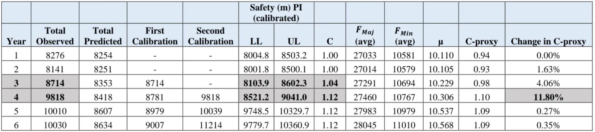
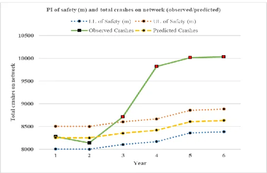
The two methodologies developed in the thesis use the uncertainty associated with the SPFs to develop the guidelines. The first methodology uses the PI of the safety (m) for the entire network and assess if the observed counts in a future year lie within the PI of the safety (m) in that year. If the observed counts are outside the PI, we need to recalibrate. The second

methodology uses the CV of the SPF and the calibration factor and evaluates the calibration factor every year. The main assumption here is that the CV of the calibration factor should not be larger than the CV of the predictive model. If it is, then the uncertainty of C is larger than that of the model, which is implies that the calibration factor is unreliable or biased. The recalibration is recommended when the calibration factor in any year is significantly different than 1. The theory behind the methodologies is described in the subsequent sections.

 

(28)

16

3.1.1 FIRST METHOD - PI OF THE SAFETY FOR THE ENTIRE NETWORK

Wood (2005) developed a methodology to calculate the confidence interval (CI) and prediction interval (PI) for a class of models known as generalized linear models (GLMs) with Poisson or NB errors. The NB model results when the safety m between sites with similar flows along with the assumption of Poisson distribution (the mean of this distribution is m) for y at a given site with safety m. This author documented a methodology for evaluating the following:

1. True accident rate μ (CI)

2. NB model – PI for safety at a new site (m) and crash rate at a new site (y). 3. Poisson model – PI for crash rate at a new site(y).

The GLMs in Wood’s study use a log link function, meaning that the logarithmic value of

μ can be expressed as a linear function of the model parameters. For example, for a model predicting the crashes with a single flow F (Wood, 2005):

𝜇 = 𝛽₀∗ 𝐹𝛽1………... (3.2) 𝜂 = log 𝜇 = log 𝛽₀+ 𝛽₁∗ 𝑙𝑜𝑔 (𝐹) = 𝛽₀′_{+ 𝛽}

1∗ 𝑙𝑜𝑔 (𝐹)……… (3.3)

Wood references the work of Dobson (1990) on the standard generalized model theory, which states that asymptotically, the estimates of 𝛽₀′ and 𝛽₁ denoted by of 𝑏₀′ and 𝑏₁ have a bivariate normal distribution.

[𝑏0

′

𝑏₁] ~ 𝑁( [ 𝛽₀′

𝛽₁] , 𝐼−1 )……….………..… (3.4)

The estimates are unbiased. The inverse of the information matrix I is the covariance matrix of the estimates. Based on the above theory, 𝜂 is asymptotically normally distributed, hence 𝜇 is approximately log normally distributed. Thus, the 95% confidence interval for 𝜂 can

(29)

17

be given by 𝜂̂ ± 1.96 ∗ √𝑉𝑎𝑟(𝜂̂) and the 95% confidence interval for 𝜇 is given by 𝑒𝜂̂±1.96∗√𝑉𝑎𝑟(𝜂̂) _: 𝑉𝑎𝑟(𝜂̂)= 𝑉𝑎𝑟(𝑏₀′ + 𝑏1 ∗ log 𝐹) = 𝑉𝑎𝑟(𝑏0′) + 2 ∗ log 𝐹 ∗ 𝐶𝑜𝑣(𝑏0′, 𝑏1) + (𝑙𝑜𝑔 𝐹)2∗ 𝑉𝑎𝑟(𝑏1) = 𝐼₁₁−1+ 2 ∗ log 𝐹 ∗ 𝐼₁₂−1+ (log 𝐹)2_{∗ 𝐼} 22−1 ……….…… (3.5) 𝜂̂ = (1, log 𝐹)(𝑏₀′, 𝑏1)𝑇 (𝑇 𝑑𝑒𝑛𝑜𝑡𝑒𝑠 𝑡𝑟𝑎𝑛𝑠𝑝𝑜𝑠𝑒)………... (3.6) 𝑉𝑎𝑟(𝜂̂) = (1, log 𝐹)𝐼−1_{(1, log 𝐹)}𝑇_{……….………... (3.7)}

where 𝐼−1 is the inverse of information matrix i.e. covariance matrix.

It should be observed that to evaluate 𝑉𝑎𝑟(𝜂̂) the covariance matrix needs to be obtained for the parameters. The statistical software used to develop the SPFs using NB regression like R, SAS have the capability of directly outputting the covariance matrix.

Wood (2005) uses the work of Maher and Summersgill (1996), who developed an approximate normal distribution for the lognormal distribution of 𝜇̂ as

𝜇̂ ~ 𝑁(𝜇0 = 𝜇, 𝜎02 = 𝜇2∗ 𝑉𝑎𝑟(𝜂̂))………...…….……… (3.8)

Wood (2005) developed the CI and PI for Poisson model and NB model. However, in the present study, only the NB model is used. Hence, only the development of CI and PI for NB is discussed.

3.1.1.1 Prediction interval for the safety (m)

Wood’s (2005) methodology uses the assumption of an approximate normal distribution of 𝜇̂, as described earlier. A gamma distribution is assumed for m; thus, to calculate the prediction interval, the gamma distribution should be mixed with a normal distribution. The mean and

(30)

18

variance of the resulting distribution are 𝜇0 and 𝜎02+ (𝜎02+ 𝜇02)/𝜙 where 𝜙 is the inverse of the

dispersion parameter. Again, assuming normality for the above distribution and substituting the values of mean and variance, the 95% PI for safety (m) is

𝜇̂ ± 1.96 ∗ √𝜇̂2_{∗ 𝑉𝑎𝑟(𝜂̂) +}𝜇̂2∗𝑉𝑎𝑟(𝜂̂)+𝜇̂2

𝜙 ………..……… (3.9)

3.1.1.2 Prediction interval for number of accidents (y)

Wood’s (2005) methodology uses the assumption of an approximate normal distribution of 𝜇̂, as described earlier. The prediction interval of the Y is calculated using a mixture of NB and a normal distribution. The mean and variance of the resulting distribution are 𝜇₀ and 𝜎₀2 +𝜎02+𝜇02

𝜙 +

𝜇₀. Wood (2005) uses Chebyshev’s one-sided inequality (Feller, 1966) to evaluate the PI for y:

𝑃(𝑌 − 𝜇_𝑌 ≥ 𝑡𝜎_𝑌) ≤_1+𝑡1₂ 𝑓𝑜𝑟 𝑡 > 0……….………. (3.10)

To evaluate the 95% confidence interval, the probability of Y exceeding the upper limit of CI should be less than 5%.

𝑡 = √19

𝑃(𝑌 ≥ 𝜇_𝑌+ √19𝜎𝑌) ≤ 1

20………... (3.11)

Lord (2008) developed a procedure for calculating the variance and CI of the product of the baseline prediction models and the CMF’s. The conventional form of the predictive model can be described as

(31)

19 where

𝜇𝑓𝑖𝑛𝑎𝑙 = 𝑓𝑖𝑛𝑎𝑙 𝑝𝑟𝑒𝑑𝑖𝑐𝑡𝑒𝑑 𝑛𝑢𝑚𝑏𝑒𝑟 𝑜𝑓 𝑐𝑟𝑎𝑠ℎ𝑒𝑠 𝑝𝑒𝑟 𝑢𝑛𝑖𝑡 𝑜𝑓 𝑡𝑖𝑚𝑒

𝜇_{𝑏𝑎𝑠𝑒𝑙𝑖𝑛𝑒} = 𝑃𝑟𝑒𝑑𝑖𝑐𝑡𝑒𝑑 𝑛𝑢𝑚𝑏𝑒𝑟 𝑜𝑓 𝑐𝑟𝑎𝑠ℎ𝑒𝑠 𝑤𝑖𝑡ℎ 𝑎𝑛 𝑆𝑃𝐹

𝐶𝑀𝐹₁∗ 𝐶𝑀𝐹₂… ∗ 𝐶𝑀𝐹_𝑛 = 𝑝𝑟𝑜𝑑𝑢𝑐𝑡 𝑜𝑓 𝐶𝑀𝐹𝑠 𝑎𝑠𝑠𝑢𝑚𝑒𝑑 𝑡𝑜 𝑏𝑒 𝑖𝑛𝑑𝑒𝑝𝑒𝑛𝑑𝑒𝑛𝑡

Lord (2008) references the work of Ang and Tang (1975) on the multiplication of the independent random variables. Let “p” be the product of the independent random variables 𝑦₁, 𝑦₂, 𝑦₃, … , 𝑦_𝑛.

𝑝 = 𝑦₁∗ 𝑦₂∗ 𝑦₃∗ … ∗ 𝑦_𝑛 Mean of the product p

𝑝 = 𝑦₁∗ 𝑦₂∗ 𝑦₃∗ … ∗ 𝑦_𝑛

𝐸[𝑝] = 𝐸[𝑦₁] ∗ 𝐸[𝑦₂] ∗ 𝐸[𝑦₃] ∗ … ∗ 𝐸[𝑦_𝑛]……… (3.13)

𝜆_𝑝 = 𝜆_𝑦1∗ 𝜆_𝑦2∗ 𝜆_𝑦3∗ … … ∗ 𝜆_𝑦𝑛

Variance of the product p

𝑝2 = 𝑦₁2∗ 𝑦₂2∗ … .∗ 𝑦_𝑛2 𝐸[𝑝2] = 𝐸[𝑦₁2] ∗ 𝐸[𝑦₂2] ∗ … .∗ 𝐸[𝑦𝑛2] (𝜆_𝑝2 _{+ 𝑣} 𝑝) = (𝜆2𝑦1+ 𝑣𝑦1) ∗ (𝜆2𝑦2+ 𝑣𝑦2) ∗ … . . (𝜆𝑦𝑛2 + 𝑣𝑦𝑛) 𝑣_𝑝 = (𝜆_𝑦12 + 𝑣_𝑦1) ∗ (𝜆_𝑦22 + 𝑣_𝑦2) ∗ … . . (𝜆_𝑦𝑛2 _{+ 𝑣} 𝑦𝑛) − 𝜆𝑝2……… (3.14)

(32)

20

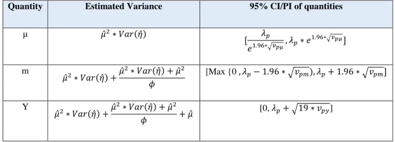
The variance of the parameters of the baseline model was evaluated earlier by Wood (2005), and the methodology to evaluate the variance with the CMFs is described in Lord (2008). In summary, the variance and the 95% PI of the parameters are given in Table 1.

Table 1. Summary of the estimated variance and 95% CI/PI for the quantities Reprinted with permission from Elsevier (Lord, 2008)

Quantity Estimated Variance 95% CI/PI of quantities

μ 𝜇̂2_{∗ 𝑉𝑎𝑟(𝜂̂)} [ 𝜆𝑝 𝑒1.96∗√𝑣𝑝μ, 𝜆𝑝∗ 𝑒 1.96∗√𝑣𝑝𝜇_] m 𝜇̂2_{∗ 𝑉𝑎𝑟(𝜂̂) +}𝜇̂ 2_{∗ 𝑉𝑎𝑟(𝜂̂) + 𝜇̂}2 𝜙 [Max {0 , 𝜆𝑝− 1.96 ∗ √𝑣𝑝𝑚), 𝜆𝑝+ 1.96 ∗ √𝑣𝑝𝑚] Y 𝜇̂2_{∗ 𝑉𝑎𝑟(𝜂̂) +}𝜇̂ 2_{∗ 𝑉𝑎𝑟(𝜂̂) + 𝜇̂}2 𝜙 + 𝜇̂ [0, 𝜆𝑝+ √19 ∗ 𝑣𝑝𝑦]

This methodology considers the entire network and evaluates the total number of observed crashes and predicted crashes (y). Similarly, it also evaluates the sum of the safety (m), the variance associated with the safety, and the variance of the predicted value y. The variance can be directly summed since the values of the parameters (m, y) at each site are independent of other sites.

(33)

21

The distribution of the sum of the parameters must be investigated to calculate the PIs of the sums. The central limit theorem (CLT) states that the mean and the sum of a random sample from an arbitrary distribution have an approximately normal distribution when the sample size is sufficiently large (Kwak and Kim, 2017). It can be represented as

𝑆𝑢𝑚 𝑜𝑓 𝑡ℎ𝑒 𝑚𝑒𝑎𝑛(𝑥𝑖)~𝑁𝑜𝑟𝑚𝑎𝑙(𝑆𝑢𝑚(𝑥𝑖), 𝑆𝑢𝑚(𝑉𝑎𝑟(𝑥𝑖))………. (3.15)

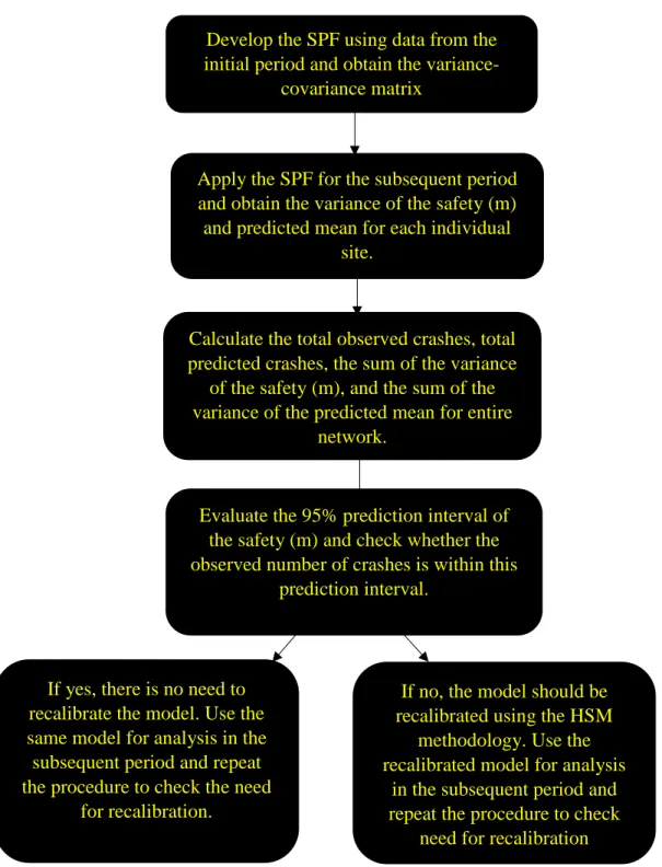
3.1.1.3Steps in the first method

Based on the above discussion, the first method is divided into the following four steps: • Develop the SPF (flow-only model ignoring the effect of other traffic and geometric

variables) using data from the initial period and obtain the variance-covariance matrix for this SPF.

• Apply the SPF to the entire network in the subsequent period and evaluate the variance of the safety (m) and the predicted number of crashes for each of the individual sites. • Compute the total observed number of crashes for the entire network, the total predicted

number of crashes (using the latest calibrated model), the sum of the variance of the safety (m), and the sum of the variance of the predicted mean for the entire network. • Evaluate the 95% PI of the safety (m). The model should be recalibrated when the

observed number of crashes is outside this PI. If it is not, use the same model in the subsequent analysis period.

• Repeat the same procedure for the subsequent time periods (using the model last recalibrated) to check the need for recalibration.

(34)

22

Figure 1. Flow chart for the first methodology proposed for recalibration Develop the SPF using data from the

initial period and obtain the variance-covariance matrix

Apply the SPF for the subsequent period and obtain the variance of the safety (m) and predicted mean for each individual

site.

Calculate the total observed crashes, total predicted crashes, the sum of the variance

of the safety (m), and the sum of the variance of the predicted mean for entire

network.

Evaluate the 95% prediction interval of the safety (m) and check whether the observed number of crashes is within this

prediction interval.

If yes, there is no need to recalibrate the model. Use the same model for analysis in the subsequent period and repeat the procedure to check the need

for recalibration.

If no, the model should be recalibrated using the HSM

methodology. Use the recalibrated model for analysis

in the subsequent period and repeat the procedure to check

(35)

23

3.1.2 SECOND METHOD: STATISTICAL DIFFERENCE OF C-FACTOR ESTIMATE The second method developed in this thesis requires an evaluation of the standard deviation of the C-factor estimate. The procedure to evaluate the coefficient of variation (CV) of the C-factor is adopted from the concept proposed by Dr. Hauer in the NCHRP report by Bahar (2014). The predicted value of the SPF can be expressed as a product of three factors:

𝑁_𝑃𝑟𝑒 = 𝑁_{𝐵𝑎𝑠𝑒}∗ 𝐶𝑀𝐹 ∗ 𝐶 𝑁 = 𝐴 ∗ 𝐵 ∗ 𝐶 𝑉{𝑁} ≅ (𝐵 × 𝐶)2∗ 𝑉{𝐴} + (𝐴 × 𝐶)2∗ 𝑉{𝐵} + (𝐴 × 𝐵)2∗ 𝑉{𝐶} … … … (3.15) Dividing by 𝑁2 𝑉{𝑁} 𝑁2 ≅ 𝑉{𝐴} 𝐴2 + 𝑉{𝐵} 𝐵2 + 𝑉{𝐶} 𝐶2 … … … (3.16) (𝑐𝑣 {𝑁_𝑝𝑟𝑒})2= (𝑐𝑣 {𝑁𝑏𝑎𝑠𝑒𝑆𝑃𝐹})2+ (𝑐𝑣{𝐶𝑀𝐹𝑠})2+ (𝑐𝑣{𝐶})2………... (3.17)

Flow-only models are developed in this methodology, and the effect of other traffic and geometric variables is ignored. Hence, the effect of the CMFs is ignored.

(𝑐𝑣 {𝑁_𝑝𝑟𝑒})2= (𝑐𝑣 {𝑁𝑏𝑎𝑠𝑒𝑆𝑃𝐹})2+ (𝑐𝑣{𝐶})2………. (3.18)

In the current methodology, the above equation condenses to when the base model is made equal to the predicted model (since the method does not use CMFs).

𝑉𝑎𝑟(𝑁_𝑝𝑟𝑒)

𝑁_𝑝𝑟𝑒2 =

𝑉𝑎𝑟(𝐶)

𝐶2 … … … (3.19)

The variance and the standard deviation of the C-factor estimate can be evaluated using the above equation.

(36)

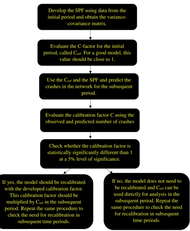
24 3.1.2.1Steps in the second method

The second method is divided into the following five steps:

• Develop the SPF (flow-only model, ignoring the effect of other traffic and geometric

variables) and calculate the C-factor for Year 1, called Cref. If a good model is developed, this

value is expected to be close to 1 (use the data of the entire network to evaluate the calibration factor).

• Adjust the estimates in Year 2 using Cref. Calculate the variances of the model estimate.

Assume that the entire variance in the model estimate is due to the variance of C. The

variance of the model estimates is obtained using the methodology proposed by Wood (2005) and Lord (2008). Estimate the calibration factor in Year 2, called 𝐶2.

• The CV of the C-factor in Year 2 is now known. Calculate the standard deviation in Year 2 as (CV of C-factor in Year 2) * (C-factor estimate of Year 2), called 𝜎.

• Test the hypothesis that the C-factor in Year 2 is significantly different than 1 at a 5% level of significance:

𝐻0: 𝐶−𝑓𝑎𝑐𝑡𝑜𝑟=1 𝐻1: 𝐶−𝑓𝑎𝑐𝑡𝑜𝑟≠1

𝑡 = 𝐶2− 1 σ

• If the null hypothesis cannot be rejected, repeat the same procedure for Year 3 using the C-factor developed in Year 1 (𝐶𝑟𝑒𝑓) for Year 3.

• If the null hypothesis is rejected, the model needs to be recalibrated in Year 2. Use the C-factor developed in Year 2 (𝐶2) and multiply it by𝐶𝑟𝑒𝑓to analyze the Year 3 data.

• Repeat the same procedure for the subsequent time periods to check the need for recalibration.

(37)

25

The flowchart in Figure 2 indicates the second methodology described in the thesis.

Figure 2. Flow chart for the second methodology proposed for recalibration Develop the SPF using data from the

initial period and obtain the variance-covariance matrix.

Evaluate the C-factor for the initial period, called Cref. For a good model, this

value should be close to 1.

Use the Cref and the SPF and predict the

crashes in the network for the subsequent period.

Evaluate the calibration factor C using the observed and predicted number of crashes

Check whether the calibration factor is statistically significantly different than 1

at a 5% level of significance.

If yes, the model should be recalibrated with the developed calibration factor.

This calibration factor should be multiplied by Cref in the subsequent

period. Repeat the same procedure to check the need for recalibration in

subsequent time periods.

If no, the model does not need to be recalibrated and Cref can be

used directly for analysis in the subsequent period. Repeat the same procedure to check the need

for recalibration in subsequent time periods.

(38)

26 3.2 SELECTING THE DATASETS

The selection of the datasets is critical in this study, since the first step involves developing an SPF with the base condition data. Moreover, the data should be available over several years to test the different calibration strategies to determine which one works the best. The methodology developed in the present study was tested using the following datasets.

Intersection Data

• Toronto 4-legged intersections (6-year dataset)

• Michigan 3-legged intersections (5-year dataset)

• Michigan 4-legged intersections (5-year dataset) Segment Data

• Michigan 2-lane undivided highways (5-year dataset)

• Michigan 4-lane undivided roads (5-year dataset)

• Michigan 4-lane divided roads (5-year dataset) 3.2.1 CHARACTERISTICS OF THE DATASETS

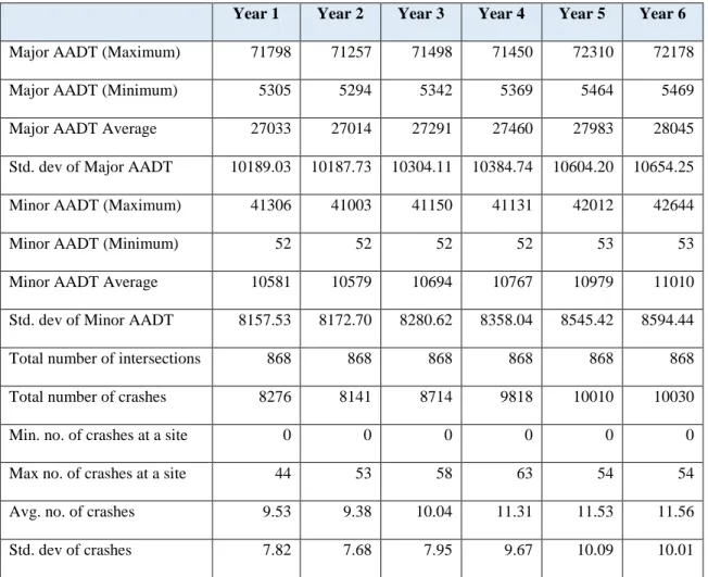
This section provides the summary statistics of the datasets used in the study 3.2.1.1 Toronto 4-legged intersections

Crash data and entering traffic flows were collected at 868 4-legged signalized intersections in Toronto for a period of 6 years. This dataset has been used extensively by other researchers (Lord, 2000; Miaou and Lord, 2003; Lord and Persaud 2004). The summary statistics for the Toronto 4-legged intersections are presented in Table 2.

(39)

27

Table 2. Summary statistics of the Toronto 4-legged intersections data Year 1 Year 2 Year 3 Year 4 Year 5 Year 6

Major AADT (Maximum) 71798 71257 71498 71450 72310 72178 Major AADT (Minimum) 5305 5294 5342 5369 5464 5469 Major AADT Average 27033 27014 27291 27460 27983 28045 Std. dev of Major AADT 10189.03 10187.73 10304.11 10384.74 10604.20 10654.25 Minor AADT (Maximum) 41306 41003 41150 41131 42012 42644

Minor AADT (Minimum) 52 52 52 52 53 53

Minor AADT Average 10581 10579 10694 10767 10979 11010 Std. dev of Minor AADT 8157.53 8172.70 8280.62 8358.04 8545.42 8594.44 Total number of intersections 868 868 868 868 868 868 Total number of crashes 8276 8141 8714 9818 10010 10030

Min. no. of crashes at a site 0 0 0 0 0 0

Max no. of crashes at a site 44 53 58 63 54 54

Avg. no. of crashes 9.53 9.38 10.04 11.31 11.53 11.56 Std. dev of crashes 7.82 7.68 7.95 9.67 10.09 10.01

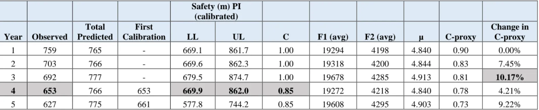
3.2.1.2 Michigan 3-legged intersections

The crash data along with the flows has been collected at 3-legged signalized intersections in Michigan for a period of five years. Entering traffic flow and crash data were collected at 174 intersections for each of the five years. The summary statistics for Michigan 3-legged

(40)

28

Table 3. Summary statistics for Michigan 3-legged intersections data

Year 1 Year 2 Year 3 Year 4 Year 5 Major AADT (Maximum) 61492 61662 61372 59046 62094

Major AADT (Minimum) 4652 4650 4625 4482 4391

Major AADT Average 19294 19318 19677 19272 19608 Std. dev of Major AADT 10196.28 10228.04 10269.17 9930.02 10349.57 Minor AADT (Maximum) 42413 42530 42330 40726 42828

Minor AADT (Minimum) 48 47 49 47 50

Minor AADT Average 4198 4200 4285 4218 4295

Std. dev of Minor AADT 5168.34 5180.83 5240.91 5107.57 5274.67 Total number of intersections 174 174 174 174 174

Total number of crashes 759 703 692 653 627

Min. no. of crashes at a site 0 0 0 0 0

Max no. of crashes at a site 30 20 21 22 27

Avg. no. of crashes 4.36 4.04 3.98 3.75 3.60

Std. dev of crashes 4.29 3.56 3.85 3.68 3.74

3.2.1.3 Michigan 4-legged intersections

The crash data along with the flows has been collected at 4-legged signalized intersections in Michigan for a period of five years. Entering traffic flow and crash data were collected at 349

(41)

29

intersections for each of the five years. The summary statistics for Michigan 4-legged intersections are presented in Table 4.

Table 4. Summary statistics for Michigan 4-legged intersections data

Year 1 Year 2 Year 3 Year 4 Year 5 Major AADT (Maximum) 120082 118318 118771 116295 117627

Major AADT (Minimum) 4033 4087 4265 4114 4164

Major AADT Average 20889 20997 21445 21078 21380 Std. dev of Major AADT 15243.17 15013.86 15223.39 15027.13 15248.81 Minor AADT (Maximum) 66148 66135 69321 68508 68487

Minor AADT (Minimum) 88 92 94 94 99

Minor AADT Average 8781 8832 9034 8870 8992

Std. dev of Minor AADT 7915.43 7905.12 8104.12 7978.87 8086.98 Total number of intersections 349 349 349 349 349 Total number of crashes 2925 2872 2989 2965 2914

Min. no. of crashes at a site 0 0 0 0 0

Max no. of crashes at a site 61 53 51 46 44

Avg. no. of crashes 8.38 8.23 8.56 8.49 8.35

(42)

30 3.2.1.4 Michigan 2-lane undivided segments

The crash data along with the flows, segment length has been collected on 2-lane undivided segments in Michigan for a period of five years. The summary statistics for Michigan 2-lane undivided segments are presented in Table 5.

Table 5. Summary statistics for Michigan 2-lane undivided segments data Year 1 Year 2 Year 3 Year 4 Year 5 Segment AADT (Maximum) 30145 28494 25327 26158 26786

Segment AADT (Minimum) 326 318 234 237 253

Segment AADT Average 8483 8202 8322 8362 8486 Std. dev of Segment AADT 5066.95 4858.89 4860.47 4977.79 5055.11 Segment Length (Max in mil.) 5.63 5.63 5.63 5.63 5.63 Segment Length (Min in mil.) 0.013 0.013 0.013 0.013 0.013 Segment Length Avg. (in mil.) 0.948 0.945 0.943 0.941 0.941 Std. dev of Segment Length 0.83 0.83 0.84 0.86 0.86

Total number of segments 471 458 450 397 397

Total Segment Length (in mil.) 446.64 432.86 424.7 373.4 373.4 Total number of crashes 1960 1680 1561 1443 1558

Min. no. of crashes/ segment 0 0 0 0 0

Max no. of crashes/ segment 65 34 32 28 80

Avg. no. of crashes 4.16 3.67 3.47 3.63 3.92

(43)

31 3.2.1.5 Michigan 4-lane undivided segments

The crash data along with the flows, segment length has been collected on 4-lane undivided segments in Michigan for a period of five years. The summary statistics for Michigan 4-lane undivided segments are presented in Table 6.

Table 6. Summary statistics for Michigan 4-lane undivided segments data Year 1 Year 2 Year 3 Year 4 Year 5 Segment AADT (Maximum) 40830 40013 36142 36612 43824 Segment AADT (Minimum) 3981 3961 3700 3748 3849 Segment AADT Average 14157 13925 13922 14013 14117 Std. dev of Segment AADT 6004.43 5687.75 5738.18 6007.46 6162.67 Segment Length (Max in mil.) 5.247 5.247 5.247 5.247 5.247 Segment Length (Min in mil.) 0.009 0.009 0.009 0.009 0.009 Segment Length Avg. (in mil.) 0.707 0.705 0.712 0.700 0.700 Std. dev of Segment Length 0.59 0.59 0.60 0.56 0.56

Total Segment Length (in mil.) 164.81 162.78 155.88 145.75 145.75

Total number of crashes 748 822 762 680 712

Avg. no. of crashes 3.21 3.56 3.48 3.27 3.42

(44)

32 3.2.1.6 Michigan 4-lane divided segments

The crash data along with the flows, segment length has been collected on 4-lane divided segments in Michigan for a period of five years. The summary statistics for Michigan 4-lane divided segments are presented in Table 7.

Table 7. Summary statistics for Michigan 4-lane divided segments data Year 1 Year 2 Year 3 Year 4 Year 5 Segment AADT (Maximum) 35184 35536 35820 34064 34881 Segment AADT (Minimum) 1855 1873 1888 1964 2011 Segment AADT Average 10071 9898 9989 10043 10185 Std. dev of Segment AADT 5683.05 5670.59 5603.15 5602.36 5575.98 Segment Length (Max in mil.) 5.143 5.143 5.143 5.143 5.143 Segment Length (Min in mil.) 0.016 0.016 0.016 0.016 0.016 Segment Length Avg. (in mil.) 0.99 0.99 0.99 0.96 0.96 Std. dev of Segment Length 0.75 0.75 0.75 0.73 0.73

Total Segment Length (in mil.) 369.49 368.82 367.95 334.63 334.63 Total number of crashes 1396 1354 1218 1334 1444

Avg. no. of crashes 3.74 3.64 3.28 3.84 4.16

(45)

33

3.3 APPLYING THE CALIBRATION METHODOLOGY

The first step of both the methodologies involves developing an SPF with flow-only data, which may or may not reflect the base conditions. The NB regression model is used to this end. The SPF can be developed using any statistical package, such as R (2014), SAS (2008), etc. In this study, it is necessary to obtain the covariance matrix between the parameters to calculate the variance associated with the SPFs. Furthermore, the inverse of the dispersion parameter is needed to evaluate the variance. The two methodologies described earlier are applied for the recalibration of the models over time. The results of both the methodologies are also compared to those of the methodology described in the HSM and the one described by Shirazi et al. (2017). 3.3.1 MODEL FORM OF THE SPFS

The initial step of both the methodologies described in the thesis is to develop an SPF for the specific facility type using the NB regression model. The selection of an appropriate model form is important since the relationship between the number of crashes and the predictive variables should be appropriately captured. Moreover, the model form also affects the results of the prediction, and thus the analysis. Researchers have studied different model forms for intersections and segments in the past.

3.3.1.1 Intersection predictive model form

Miaou and Lord (2003) indicate that several model forms for intersection SPFs are possible even when very few covariates are considered. They state that when an appropriate model form must be chosen several factors should be considered engineering logics, exploratory data analysis, the flow values available, the covariate data, and the crash data. The authors reference the work of Turner and Nicholson, who classified the intersection model forms into three types. The Type 1

(46)

34

models relate the total number of crashes to the traffic volumes entering the intersection; the Type 2 models relate the crashes to two flows approaching from the major and minor roads, respectively; and the Type 3 models the number of crashes involving conflicting movements of vehicles. The Type 3 models require the maximum amount of data with detailed turning flows and number of crashes by movement group.

The most commonly used are the Type 2 models. The authors indicated that the Type 2 models follow the logic of no flow, no crashes, and they allow a nonlinear relationship between crashes and flows (this relationship has been found to be representative based on several studies in the past). The model form in the HSM is also a Type 2 model. The present study uses a Type 2 model with the model form shown in Equation 25.

𝜇 = 𝛽₀∗ 𝐹_𝑀𝑎𝑗𝛽1 _{∗ 𝐹}

𝑀𝑖𝑛

𝛽2 _{… … … . (3.20)}

where FMaj, FMin are the entering flows (AADT) on major and minor streets, respectively.

In the present study, flow-only models are developed, ignoring the effects of the other traffic and geometric variables.

3.3.1.2 Segment predictive model form

The probability of a crash in a segment depends on the traffic flow and the length of the segment. The exploratory data analysis and engineering judgement based on several past studies indicate a nonlinear relationship between crashes and flow. For the selected functional form, the crash risk per unit length does not depend on the segment length, and the segment length (L) is therefore considered an offset in the modeling process. The model form is shown in Equation 26.

(47)

35 3.4 CHAPTER SUMMARY

This chapter has described the theory behind both the methodologies proposed for the recalibration procedure and described the steps that a practitioner or safety analyst needs to follow to apply both these methodologies. The chapter also presented a summary of the three intersection datasets and three segment datasets used to test the methodologies, and described the model form of the SPFs developed for intersections and segments.

(48)

36

CHAPTER IV

ANALYSIS RESULTS: FIRST METHOD

This chapter presents the results of applying the first method for recalibration to the datasets listed above. These results are compared to those of the methodology proposed in Shirazi et al. (2017). The chapter is divided into six sections. Section 4.1 describes the results of Toronto legged intersections. Sections 4.2 and 4.3 then describe the results of Michigan 3-legged and 4-legged intersections. Finally, Sections 4.4, 4.5, and 4.6 describe the results of Michigan 2-lane undivided, 4-lane undivided, and 4-lane divided segments, respectively.

4.1 TORONTO 4-LEGGED INTERSECTIONS

The statistical software R was used to fit the safety performance function using the NB

regression. The model was fit using the data of the first year, and was then recalibrated over time based on the two methodologies. The parameters of the model fit are presented in Table 8, and the variance-covariance matrix is presented in Table 9.

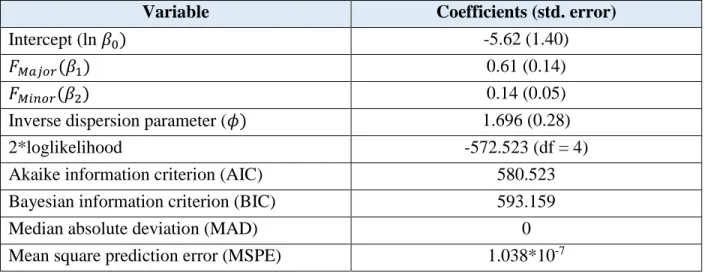
Table 8. Model output for the Toronto 4-legged intersections

Variable Coefficients (std. error)

Intercept (ln 𝛽0) -8.84 (0.48)

𝐹𝑀𝑎𝑗𝑜𝑟(𝛽1) 0.51 (0.05)

𝐹𝑀𝑖𝑛𝑜𝑟(𝛽2) 0.64 (0.02)

Inverse dispersion parameter (𝜙) 6.77 (0.62)

2*loglikelihood -4873.968 (df = 4)

Akaike information criterion (AIC) 4881.968 Bayesian information criterion (BIC) 4901.033

Median absolute deviation (MAD) 1.007