Extending the Human Connectome Project across ages: Imaging protocols for the Lifespan Development and Aging projects
Michael P. Harms*a, Leah H. Somerville*f,g, Beau M. Ances b, Jesper Anderssonh, Deanna M. Barcha,c,e, Matteo Bastianih, Susan Y. Bookheimerk, Timothy B. Brownc, Randy L. Bucknerf,g,m,n, Gregory C. Burgessa, Timothy S. Coalsond, Michael A. Chappell h,i, Mirella Daprettok, Gwenaëlle Douaudh, Bruce Fischlm,o, Matthew F. Glasserc,d,p , Douglas N. Grevem, Cynthia Hodgea, Keith W. Jamisonq, Saad Jbabdih, Sridhar Kandalaa, Xiufeng Li r, Ross W. Mairg,m, Silvia Mangiar, Daniel Marcusc, Daniele Mascalit, Steen Moellerr, Thomas E. Nicholsh,j,u, Emma C. Robinsonv, David H. Salatm, Stephen M. Smithh, Stamatios N. Sotiropoulos h,w, Melissa Terpstrar, Kathleen M.
Thomass, M. Dylan Tisdallx, Kamil Ugurbilr, Andre van der Kouwem,n, Roger P. Woodsk,l, Lilla Zölleim, David C. Van Essend, & Essa Yacoubr
* Equal first author contribution
Departments of Psychiatry a, Neurology b, Radiology c, and Neuroscience d, Washington University School of Medicine, St. Louis, MO USA
Department of Psychological and Brain Sciences e, Washington University in St. Louis, St. Louis, MO USA
Department of Psychologyf and Center for Brain Scienceg, Harvard University, Cambridge, MA USA Wellcome Centre for Integrative Neuroimaging, Oxford Centre for Functional Magnetic Resonance
Imaging of the Brain (FMRIB), Nuffield Department of Clinical Neurosciences h, University of Oxford, Oxford, UK
Institute of Biomedical Engineering, Department of Engineering Science i, University of Oxford, Oxford,
UK
Oxford Big Data Institute, Li Ka Shing Centre for Health Information and Discovery, Nuffield Department of Population Healthj, University of Oxford, Oxford, UK
Departments of Psychiatry and Biobehavioral Sciences k and Neurology l, David Geffen School of Medicine at UCLA, University of California, Los Angeles, CA USA
Athinoula A. Martinos Center for Biomedical Imaging, Department of Radiology m and Department of Psychiatryn, Massachusetts General Hospital, Harvard Medical School, Boston, MA USA
Computer Science and Artificial Intelligence Laboratory o, Massachusetts Institute of Technology, Cambridge, MA USA
St. Luke’s Hospitalp, St. Louis, MO USA
Department of Radiologyq, Weill Cornell Medical College, New York, NY USA
Center for Magnetic Resonance Imaging r and Institute of Child Development s, University of Minnesota, Minneapolis, MN USA
Centro Fermi - Museo Storico della Fisica e Centro Studi e Ricerche “Enrico Fermi”t, Rome, Italy Department of Statisticsu, University of Warwick, Coventry, UK
Department of Biomedical Engineeringv, King’s College London, London, UK
Sir Peter Mansfield Imaging Centrew, School of Medicine, University of Nottingham, Nottingham, UK Department of Radiology x, Perelman School of Medicine, University of Pennsylvania, Philadelphia, PA
US
Corresponding author: Michael Harms
Department of Psychiatry Campus Box 8134 660 South Euclid Ave. St. Louis, MO 63110
ABSTRACT
The Human Connectome Projects in Development (HCP-D) and Aging (HCP-A) are two large-scale brain imaging studies that will extend the recently completed HCP Young-Adult (HCP-YA) project to nearly the full lifespan, collecting structural, resting-state fMRI, task-fMRI, diffusion, and perfusion MRI in participants from 5 to 100+ years of age. HCP-D is enrolling 1300+ healthy children, adolescents, and young adults (ages 5-21), and HCP-A is enrolling 1200+ healthy adults (ages 36-100+), with each study collecting longitudinal data in a subset of individuals at particular age ranges. The imaging protocols of the HCP-D and HCP-A studies are very similar, differing primarily in the selection of different task-fMRI paradigms. We strove to harmonize the imaging protocol to the greatest extent feasible with the completed HCP-YA (1200+ participants, aged 22-35), but some imaging-related changes were motivated or necessitated by hardware changes, the need to reduce the total amount of scanning per participant, and/or the additional challenges of working with young and elderly populations. Here, we provide an overview of the common HCP-D/A imaging protocol including data and rationales for protocol decisions and changes relative to HCP-YA. The result will be a large, rich, multi-modal, and freely available set of consistently acquired data for use by the scientific community to investigate and define normative developmental and aging related changes in the healthy human brain.
Keywords: connectomics, resting-state, functional connectivity, task, diffusion, perfusion, development, aging, lifespan
Highlights:
● The Lifespan Human Connectome Projects in Development and Aging (HCP-D/A) are large-scale brain imaging projects that aim to characterize brain connectivity changes in human childhood and aging.
● Here, we report on the multimodal brain imaging protocol being used for both projects, and explain how the protocols differ from the related Human Connectome Project which focused on young adults.
● We report pilot and ancillary data that informed the selection of hardware and imaging parameters, which yield high quality data within the pragmatic constraints associated with imaging these populations.
● These data will be publicly released in unprocessed and minimally processed formats.
CONTENTS
1. INTRODUCTION 5
1.1. Relation to HCP-Young Adult Project 5
1.2. Harmonization across sites 6
2. MRI HARDWARE 7
3. IMAGE ACQUISITION 9
3.1. T1w and T2w structural imaging 13
3.2. BOLD imaging 14
3.2.1 Multiband multi-echo piloting 15
3.2.2. Resting state fMRI 18
3.2.3. Task fMRI 18
3.3. Diffusion imaging 19
3.4. Perfusion imaging 22
3.5. Ancillary data collected during scan session 25
3.5.1. Pulse oximetry and respiration 25
3.5.2. Eye monitoring 25
4. INFORMATICS AND PUBLIC RELEASE 25
5. CONCLUSION 27
1. INTRODUCTION
A growing number of large-scale neuroimaging studies have contributed to recent progress in deciphering human brain structure, function, and connectivity. One such endeavor is the Human Connectome Project (HCP), a pair of NIH-funded consortia that refined existing methods, developed new methods, and acquired foundational data to characterize brain networks in healthy young adults aged 22-35 {Fan, 2016 #3111;Glasser, 2013 #2892;Glasser, 2016 #3197;Glasser, 2016 #3211;Van Essen, 2013 #3347;Smith, 2013 #2815;Setsompop, 2013 #3404}. The success of this ‘Young-Adult’ HCP (HCP-YA), prompted NIH to launch the Lifespan Human Connectome Projects, which include three consortia that collectively target the human postnatal lifespan using “HCP-style” data acquisition, analysis, and sharing. Here, we provide an introduction and overview to the many aspects of the imaging protocols that are common to two of these projects -- the Lifespan Human Connectome Projects in Development (HCP-D) and in Aging (HCP-A) [ http://www.humanconnectome.org], which were both funded under the auspices of the NIH Blueprint for Neuroscience Research, starting in the summer of 2016 . We include analyses of imaging data that help to frame the imaging protocol in the1 context of HCP-YA and justify the protocol choices. Separate publications address aspects that are unique to the HCP-D project {Somerville, 2018 #3451} and the HCP-A project {Bookheimer, under review #3452}.
A major consideration in planning the imaging protocol for HCP-D/A was the challenges particular to scanning younger and older populations. These include an increased tendency for head motion at both younger {Satterthwaite, 2012 #2734} and older ages {Mowinckel, 2012 #3063;Geerligs, 2017 #3281}, coupled with a reduced tolerance for long individual scans and long overall scan sessions (e.g., due to boredom and reduced compliance at younger ages, and muscular or joint discomfort or other medical comorbidities at older ages). Key decisions about MRI hardware and protocol design were made with these challenges in mind. Thus, a common theme of this paper is how to manage the challenges of imaging a diverse span of ages in a harmonized but optimal manner.
1.1. Relation to HCP-Young Adult Project
The HCP-D and HCP-A protocols were strongly influenced by the original HCP Young Adult (HCP-YA) Project, for which data acquisition was conducted at Washington University (3T customized ‘Connectom’ scanner) and the University of Minnesota (7T scanner) from 2010-2016 {Van Essen, 2013 #3347}. Thus, many common data components exist between the HCP-D, HCP-A, and HCP-YA projects. First, both HCP-D and HCP-A include the same imaging modalities as collected in the HCP-YA: structural imaging (T1w and T2w; sMRI), diffusion imaging (dMRI), resting state functional connectivity (rfMRI), and task-based functional imaging (tfMRI). However, a different scanner platform was used and various
1 The third component of the NIH-funded Lifespan Human Connectome Project is the “Baby Connectome” project, which spans ages 0 to 5 years and uses data acquisition and analysis customized for very young children [http://babyconnectomeproject.org].
changes were made to the imaging protocols in order to customize the HCP-D/A projects to the scientific and pragmatic needs of their specific study populations (see Imaging Acquisition ). The HCP-YA imaging data were acquired over two days in four sessions of ~1-hour each, which exceeds the tolerance of many younger children and older adults. Hence, we shortened the duration for each modality. We modified the task fMRI to make the tasks maximally informative about functional domains of high interest for each lifespan stage. We also maximized the similarity of the HCP-D, HCP-A, and HCP-YA out-of-scanner assessments, although some of the behavioral assessments are only appropriate for limited age ranges {see \Somerville, 2018 #3451;Bookheimer, under review #3452} for details on the behavioral assessments of each individual project).
The NIH Funding Opportunity Announcements for HCP-D and HCP-A excluded the 22-35 years age range under the rationale that the young adult age range was already well sampled by the HCP-YA project. This poses challenges for bridging the full lifespan across the HCP-D, HCP-A, and HCP-YA projects, since the 3T data for HCP-YA were collected on a customized ‘Connectom’ scanner using a longer scan protocol and modestly different scan parameters. In contrast, scanning for HCP-D and HCP-A is conducted on standard Siemens 3T Prisma scanners. Thus, work is needed to determine the degree to which the data can be merged across projects, as well as with other large-scale projects. To aid in addressing this issue, we have acquired data on the HCP-D/A and HCP-YA platforms in the same 17 participants (see Section 2.1 , MRI Scanner ). These scans will be analyzed and made publicly available to enable systematic analysis of the impact of hardware and protocol differences, and to enable users to investigate approaches for maximally harmonizing and jointly analyzing HCP-D and HCP-A with the extensive young-adult data collected by the HCP-YA study. Additionally, data from more than 100 healthy subjects in the 22-35 age range, scanned using protocols very similar to ours, will be made available via the NIH-funded Connectomes Related to Human Disease projects. We will also facilitate harmonization with the brain imaging component of the UK Biobank prospective epidemiological study {Miller, 2016 #3200} [http://imaging.ukbiobank.ac.uk], which has an imaging target of 100,000 participants, by scanning 20 participants from the HCP-A project through the Biobank imaging protocol on a standard Siemens 3T Skyra scanner at the Athinoula A. Martinos Center for Biomedical Imaging at Massachusetts General Hospital (which is the same model scanner being used for the Biobank project).
1.2. Harmonization across sites
To meet the HCP-D/A recruitment and diversity goals, data are currently being acquired at four different institutions for each project . All scanning is conducted on a common platform 2 across sites running the same software version (E11C) using an electronically distributed protocol. One volunteer served as a “human phantom” who was scanned at each site twice
2 HCP-D data acquisition is conducted at Harvard University, University of California-Los Angeles, University of Minnesota and Washington University in St. Louis. For HCP-A, Massachusetts General Hospital serves as the 4 thacquisition site instead of Harvard. Additionally, investigators at the University of Oxford play a key role in guiding acquisition and data analytic approaches, as in HCP-YA.
(5-7 months apart); these data will be analyzed for site effects within a single individual. Additionally, using ongoing QC processes {Marcus, 2013 #3245;Hodge, 2016 #3138} we monitor for possible site differences in imaging measures and check for drifting or abrupt changes in measures as a function of time. Initial analyses of QC data indicate that less than 10% of variance is explained by site on QC measures derived from resting-state data such as temporal SNR, relative (frame-to-frame) motion, and image smoothness. Thus, even though there may ultimately be some statistically significant differences across sites (due to the power to detect even small differences with a large number of subjects), we anticipate that variability will be mainly attributable to non-site-specific factors. To ensure procedures are followed consistently and accurately across sites, we instituted a set of “standard operating procedures” (SOPs), training sessions, frequent cross-site communication, and evaluation visits to each site by the lead coordinator.
2. MRI HARDWARE
Scanning at all sites uses a Siemens 3T Prisma, a whole-body scanner with 80 mT/m gradients capable of a slew rate of 200 T/m/s. These gradients are the product variant of the 100 mT/m research gradients used in the customized 3T ‘Connectom’ (HCP-YA) scanner. High gradient strength is especially valuable for diffusion MRI (dMRI), as it achieves high diffusion weighting with high sensitivity {Sotiropoulos, 2013 #2991}, made possible by the much shorter echo times that can be achieved compared to previous generations of commercial gradient systems. The 32-channel head coil enables high acceleration factors via simultaneous multislice (SMS; i.e., “multiband”) acquisitions {Xu, 2013 #3115;Feinberg, 2010 #2535}, for which we are using the multiband EPI sequences available through the Center for Magnetic Resonance Research (CMRR) [ http://www.cmrr.umn.edu/multiband] . Together, these3 technologies enable whole brain imaging with submillimeter structural MRI, subsecond BOLD fMRI, high spatial resolution perfusion imaging, and high angular and spatial resolution diffusion imaging with higher signal to noise than is possible on more conventional 3T MRI scanners.
To enable analysis of the cumulative impact of hardware and protocol differences between the Prisma (HCP-D/A) and customized ‘Connectom’ (HCP-YA) scanners/protocols, 17 participants were scanned through the full HCP-YA protocol (prior to decommissioning the customized ‘Connectom’ scanner in 2016) and then enrolled in the HCP-A study. As an initial analysis of this data we computed the temporal SNR (tSNR) of the resting-state data. tSNR was very similar between the Prisma and ‘Connectom’ scanners (Figure 1), but with differences
3 Siemen’s VE11C software version introduced their implementation of SMS for fMRI and dMRI (with add-on SMS license). To our knowledge there has not yet been a rigorous comparison with the CMRR implementation. The CMRR version also includes useful features such as: (i) option to save the “single-band reference” image, (ii) option to automatically write the raw k-space data to a remote disk, (iii) more robust control of reversed phase encoding polarity, and (iv) dicom logging of physiological recordings. For these reasons, along with the breadth of experience with the CMRR sequences, including feedback from hundreds of independent investigators over the course of nearly a decade, we continue to use the CMRR implementation.
that will nonetheless need to be carefully considered for their potential to manifest as “group” differences in downstream analyses.
Figure 1 (color). Scatterplots of temporal SNR (tSNR) of surface vertices (left panel) and subcortical voxels (right panel) in the Prisma scanner (used for HCP-D and HCP-A) versus the customized ‘Connectom’ scanner (used for HCP-YA), colored according to the relative density of the points (black = low density; light yellow = highest density). tSNR maps (mean signal over time divided by the standard deviation over time) were computed for all four resting-state runs from 17 participants (age range 22-35 years; mean age=28.4; 10 females) who were scanned using both scanners/protocols (average interval: 6.4 months) after (i) processing with the HCP ‘minimal-preprocessing’ pipeline to yield a 2 mm standard grayordinate (CIFTI) representation (59412 surface vertices and 31870 ‘subcortical’ voxels, including cerebellum), (ii) truncation of the longer ‘Connectom’ rfMRI scans to a duration equivalent to the rfMRI scans collected on the Prisma (~6.4 min), and (iii) application of a Gaussian-weighted linear high-pass filter with a soft cutoff of 2000 s. Maps of tSNR were computed for every run, then median maps were computed across subjects within scanner and phase encoding direction. The resulting median maps were averaged across phase encoding directions for each scanner, and then plotted against each other here, separately for cortical vertices and subcortical voxels. Note the differing ranges of the axes between the two panels. The red diagonal line is the line of identity. The Prisma scanner data (HCP-D/A protocol) tends to have slightly higher tSNR, but also includes a slightly longer TR (see Section 3.2 BOLD Imaging), and thus more T1-recovery but fewer volumes for a given acquisition duration. tSNR was computed without any adjustment applied for these small protocol differences. The clusters of outliers both above and below the main diagonal in the subcortical panel arise from voxels at the edges of the subcortical structures that experienced different degrees of smoothing when mapping the volume into subcortical grayordinates, and should thus be ignored. Data and maps are available at https://balsa.wustl.edu/study/show/gjjZ, including tSNR maps computed separately for ‘AP’ and ‘PA’ phase encoding polarity (HCP-D/A protocol) and ‘LR’ and ‘RL’ polarity (HCP-YA protocol), which can be
visualized to appreciate the subtle spatial effects of phase encoding polarity on tSNR in the orbitofrontal and inferior temporal regions.
Participants 8-21 years old in HCP-D and all participants in HCP-A use the Siemens 32-channel Prisma head coil. See Supplemental Text for some additional details regarding this choice, including our plans for the head coil for scanning the 5-7 year olds.
3. IMAGE ACQUISITION
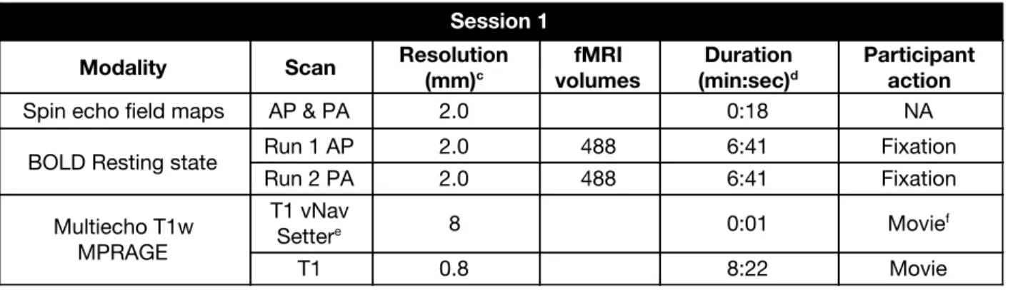
To promote consistently high data quality, to ensure participant satisfaction across the lifespan, and to accomplish that in the context of a large-scale study, it was important to reduce the total scanning from the 4 sessions of HCP-YA to 2 sessions for HCP-D/A. When designing the protocol, we targeted approximately 45 min of total scan time per session, so that most participants would be “in the bore” less than 60 min. The reduction of the alloted scanning duration by over 50% relative to HCP-YA necessitated some difficult choices. For example, while we added a perfusion scan to the HCP-D/A protocols (see below), some other potentially informative scans such as fluid attenuated inversion recovery (FLAIR) and susceptibility weighted imaging (SWI) were considered but in the end not included. Additionally, we targeted protocol adaptations that would help reduce the impact of an increased tendency for motion and/or discomfort in the youngest and oldest individuals. This includes the use of navigators and real-time motion correction in the T1w/T2w structural scans (see Section 3.1), use of a 2D (rather than 3D) sequence for ASL (Section 3.4), and generally shorter individual run durations relative to HCP-YA. Table 1 provides an overview of the imaging protocol in HCP-D and HCP-A, while Table 2 summarizes the main differences between the HCP-D/A and HCP-YA imaging protocols. The field-of-view for all scans is positioned automatically using Siemens’ AutoAlign feature (in conjunction with appropriate rotations and position offsets saved with each scan) to ensure consistent positioning and angulation across participants. A detailed listing of all scan parameters is available at http://protocols.humanconnectome.org, where an importable protocol file is also available for Siemens scanners.
Table 1. Imaging protocol for 8-100+ year-old participantsa,b
Session 1
Modality Scan Resolution (mm)
c volumes fMRI (min:sec)Duration d Participant action
Spin echo field maps AP & PA 2.0 0:18 NA
BOLD Resting state Run 1 AP 2.0 488 6:41 Fixation
Run 2 PA 2.0 488 6:41 Fixation
Multiecho T1w MPRAGE
T1 vNav
Settere 8 0:01 Movief
T2w SPACE T2 vNav Settere 8 0:01 Movie
T2 0.8 6:35 Movie
T2w TSE (HCP-A only) HighRes Hipp 0.4 x 0.4 x 2.0 3:31 Movie
Spin echo field maps AP & PA 2.0 0:18 NA
BOLD Task 1g
HCP-D: Guessing Run 1 PA 2.0 280 3:55 Task
Run 2 AP 2.0 280 3:55 Task
HCP-A: VisMotor Run 1 PA 2.0 194 2:46 Task
BOLD Task 2g
HCP-D: Go/NoGo Run 1 PA Run 2 AP 2.0 2.0 300 300 4:11 4:11 Task Task HCP-A: Go/NoGo Run 1 PA 2.0 300 4:11 Task
BOLD Task 3g
HCP-D: Emotion Run 1 PA 2.0 178 2:33 Task HCP-A: FaceName Run 1 PA 2.0 345 4:47 Task
Cumulative scan duration 45-48 min
Session 2
Modality Scan Resolution (mm)c volumes fMRI (min:sec)Duration d Participant action
Spin echo field maps AP & PA 2.0 0:18 NA
BOLD Resting state Run 1 AP 2.0 488 6:30 Fixation
Run 2 PA 2.0 488 6:30 Fixation
Spin echo field maps AP & PA 2.0 0:18 NA
Diffusion
Run 1
98 dir AP 1.5 5:38 Movie
Run 2
98 dir PA 1.5 5:38 Movie
Run 3
99 dir AP 1.5 5:42 Movie
Run 4
99 dir PA 1.5 5:42 Movie
ASL Field Map AP & PA 2.5h 0:18 NA
ASL PCASL 2.5h 5:29 Fixationi
Cumulative scan duration 43 min
a The youngest participants (5-7 years old) in HCP-D complete a slightly modified imaging protocol, which differs only in that it includes (i) three rfMRI runs per session (six in total), each consisting of 263 volumes, and (ii) a single run (PA polarity) of the Guessing and Go/NoGo tasks (which are otherwise identical).
b For conciseness, a “Localizer block”, consisting of brief localizer and AutoAlign scout scans is omitted. c Isotropic spatial resolution (voxel size), unless noted.
d Durations reflect what is listed on scanner, which includes calibration and discarded scans. For the T1w MPRAGE and T2w SPACE scans, the listed durations also include up to 80 s of k- space reacquisition.
e The “T1/T2 vNav setter” scans are very short scans that write the imaging parameters for the volumetric navigators to a file that is then read by the main T1w/T2w scans for setting the navigator parameters.
f Participant selects a movie/documentary from options provided by each site.
g HCP-D has two runs of the first two tasks (for its 8-21 year old participants), acquired with opposite phase encoding polarity; HCP-A has only a single run of all three tasks.
h Nominal slice thickness of 2.27 mm with a 10% gap (yielding 2.5 mm between slices). i The 5-7 year old participants are allowed to watch a movie during the ASL scan.
AP = anterior to posterior phase encoding direction; PA = posterior to anterior; TSE = turbo-spin-echo; ASL = arterial spin labeling; PCASL = Pseudo-continuous ASL.
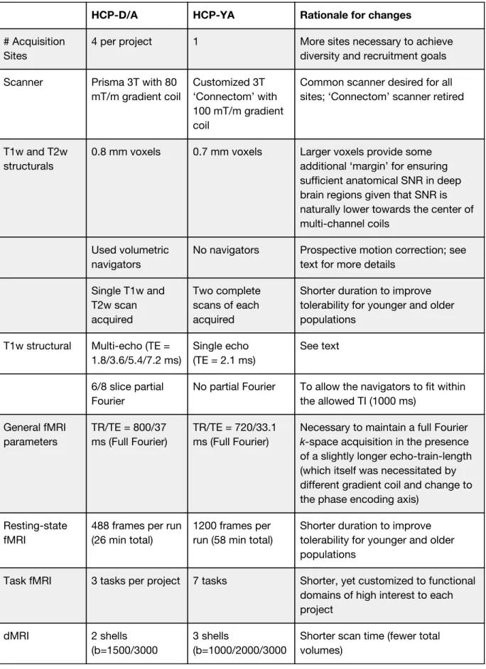
Table 2. Main differences between HCP-D/A and HCP-YA imaging protocols
HCP-D/A HCP-YA Rationale for changes
# Acquisition Sites
4 per project 1 More sites necessary to achieve diversity and recruitment goals Scanner Prisma 3T with 80
mT/m gradient coil
Customized 3T ‘Connectom’ with 100 mT/m gradient coil
Common scanner desired for all sites; ‘Connectom’ scanner retired
T1w and T2w structurals
0.8 mm voxels 0.7 mm voxels Larger voxels provide some additional ‘margin’ for ensuring sufficient anatomical SNR in deep brain regions given that SNR is naturally lower towards the center of multi-channel coils
Used volumetric
navigators
No navigators Prospective motion correction; see text for more details
Single T1w and T2w scan acquired Two complete scans of each acquired
Shorter duration to improve tolerability for younger and older populations
T1w structural Multi-echo (TE = 1.8/3.6/5.4/7.2 ms) Single echo (TE = 2.1 ms) See text 6/8 slice partial Fourier
No partial Fourier To allow the navigators to fit within the allowed TI (1000 ms) General fMRI parameters TR/TE = 800/37 ms (Full Fourier) TR/TE = 720/33.1 ms (Full Fourier)
Necessary to maintain a full Fourier k-space acquisition in the presence of a slightly longer echo-train-length (which itself was necessitated by different gradient coil and change to the phase encoding axis)
Resting-state fMRI
488 frames per run (26 min total)
1200 frames per run (58 min total)
Shorter duration to improve tolerability for younger and older populations
Task fMRI 3 tasks per project 7 tasks Shorter, yet customized to functional domains of high interest to each project
dMRI 2 shells
(b=1500/3000
3 shells
(b=1000/2000/3000
Shorter scan time (fewer total volumes)
s/mm2); 92-93 directions per shell
s/mm2); 90
directions per shell
MB=4; TR=3.23 s;
1.5 mm voxels
MB=3; TR=5.52 s; 1.25 mm voxels
Maintain sufficient diffusion SNR given the fewer total volumes (see text)
fMRI, dMRI, & Spin echo field maps
AP/PA phase encoding polarity
LR/RL polarity See text
High-resolution hippocampal
New to HCP-A
PCASL New to HCP-D and HCP-A
3.1. T1w and T2w structural imaging
The commonly used MPRAGE sequence {Mugler, 1990 #1337} was used for the T1w scan and a variable-flip-angle turbo-spin-echo (TSE) sequence (Siemens SPACE) {Mugler, 2000 #1621} for the T2w scan. High spatial resolution and the combined use of both T1w and T2w information improves the quality of surface reconstructions {Glasser, 2013 #2892;van der Kouwe, 2008 #2068} and enables generation of cortical estimates of myelin based on the T1w/T2w ratio {Glasser, 2011 #3362;Shafee, 2015 #3385}. However, for HCP-D/A we made two key changes to the acquisition methods.
First, the T1w scans use a multi-echo MPRAGE {van der Kouwe, 2008 #2068} in place of the conventional MPRAGE pulse sequence. The multi-echo version acquires 4 different echoes for each line of k -space within the same scan duration as a conventional single-echo MPRAGE scan of the same spatial resolution by using rapid switching of the readout gradient (higher bandwidth). The higher bandwidth reduces susceptibility-induced distortions, while the consequent lower SNR of the individual echo images is offset by combining the 4 echoes. The resulting root mean square (RMS)-averaged T1w image has contrast and SNR that is comparable to a normal MPRAGE. The high bandwidth also enables the bandwidth to be matched to the T2w scan, thus ensuring more precise voxel-wise registrations, benefiting cortical estimates of myelin {Shafee, 2015 #3385}.
Second, the HCP-D/A protocol includes embedded volumetric navigators (vNavs) in the T1w and T2w sequences for prospective motion correction and for selective reacquisition of the lines in k-space that are heavily corrupted by subject motion {Tisdall, 2012 #3323}. To this end, very short, low-resolution, 3D echo-planar imaging volumetric navigators are acquired once for every TR period (i.e., every ~2.5-3 s), registered in real-time, and the resulting positional information used to update the image FOV position during the scan in a similar manner to the prospective motion correction sometimes used for BOLD scanning {Thesen,
2000 #2388;Zaitsev, 2006 #3429}. Real-time motion correction can substantially reduce bias in brain morphometry results, where motion might induce measurable morphometric differences {Reuter, 2015 #2895;Tisdall, 2016 #3112}. In the HCP-D/A protocol, the vNavs are acquired with the body coil to yield a more homogenous image, and their initial position is set (automatically using AutoAlign) to exclude most of the neck, so that the registration is driven primarily by the brain. In the HCP-D/A protocols, up to 80 s of k-space reacquisition is allowed at the end of the vNav-enabled MPRAGE and SPACE scans to replace the motion-corrupted k-space lines in the final image reconstruction. This adds modestly to the maximum possible duration of the T1w and T2w scans, but is more efficient than having to re-collect an entire scan and choosing the one with less degradation due to motion. As of June 2018, fewer than 5% of the T1w and T2w scans for both HCP-D and HCP-A have been rated as ‘poor’ based on a manual quality inspection {Marcus, 2013 #3245}. The low incidence of poor structural scans in these cohorts is likely attributable to the use of the real-time motion correction and k -space reacquisition.
We also reduced the overall duration of the structural scanning by acquiring a single T1w and T2w scan, each with 0.8 mm isotropic voxels, in HCP-D/A (except when the initial scan is poor quality). Both structural scans use a sagittal FOV of 256 × 240 × 166 mm with a matrix size of 320 × 300 × 208 slices. Slice oversampling of 7.7% is used, as is 2-fold in-plane acceleration (GRAPPA) in the phase encode direction and a pixel bandwidth of 744 Hz/Px. For the T1w scan, other parameters include: TR/TI=2500/1000, TE=1.8/3.6/5.4/7.2 ms, flip angle of 8 deg, water excitation employed for fat suppression (to reduce signal from bone marrow and scalp fat), and up to 30 TRs allowed for motion-induced reacquisition. For the T2w scan, other parameters include TR/TE=3200/564 ms, turbo factor=314, and up to 25 TRs allowed for motion-induced reacquisition.
Last, given the central role of the hippocampus in studies of aging, for HCP-A we added a 2D, T2w, turbo-spin-echo scan with high in-plane resolution (0.39 x 0.39 mm) and 2 mm coronal-oblique slices oriented approximately perpendicular to the long axis of the hippocampus. This high in-plane resolution allows identification of hippocampal and amygdalar subregions {Iglesias, 2015 #3107;Saygin, 2017 #3386;Bookheimer, under review #3452}.
3.2. BOLD imaging
T2*-weighted scans sensitive to the BOLD contrast are used for resting and task-based functional MRI. The scan parameters used for the fMRI scans in HCP-D and HCP-A are very similar to those used in HCP-YA. Specifically, the fMRI scans are acquired with a 2D multiband (MB) gradient-recalled echo (GRE) echo-planar imaging (EPI) sequence (MB8, TR/TE=800/37 ms, flip angle=52 o) and 2.0 mm isotropic voxels covering the whole brain (72 oblique-axial slices). Except for certain task-fMRI acquired with a single run (see Table 1), functional scans are acquired in pairs of two runs, with opposite phase encoding polarity so that the fMRI data in aggregate is not biased toward a particular phase encoding polarity. For HCP-D/A we use anterior-to-posterior (“AP”) and posterior-to-anterior (“PA”) phase encoding rather than left-to-right (LR) and right-to-left (RL) phase encoding as used for HCP-YA {Smith, 2013 #2889}. This is because the allowable echo-spacings on the Prisma are such that one cannot
achieve a shorter overall echo-train-length when using LR/RL phase encoding compared to AP/PA, despite the smaller required L-R phase field-of-view. A pair of spin echo images with AP and PA phase encoding polarity with matching geometry and echo-spacing to the GRE scans are also acquired at the beginning and middle of each scanning session for mapping and correction of image distortions related to magnetic field inhomogeneities.
Additionally, for HCP-D/A all sites introduced Framewise Integrated Real-time MRI Monitoring (FIRMM) {Dosenbach, 2017 #3316} approximately 9 months after the onset of data collection in each project. We are using FIRMM with all BOLD scans (both resting-state and task) to provide valuable real-time feedback to the scanner operators regarding subject movement. Operators then use this information to provide feedback to participants between fMRI runs. If excessive motion is observed at the beginning of a run, that run is aborted, the participant asked if they are comfortable, and are reminded of the importance of staying still.
3.2.1 Multiband multi-echo piloting
Although the above-described parameters were ultimately adopted as the best compromise for harmonization with HCP-YA, in a piloting phase we evaluated a multi-echo (ME) fMRI sequence as an alternative to the single echo approach of the HCP-YA {Kundu, 2012 #3403;Kundu, 2013 #3369}. An ME sequence permits separation of fMRI data into TE dependent (hence a BOLD effect) and TE independent (presumed artifact) components, thereby facilitating the denoising process. However, to achieve the same spatial resolution, the acquisition of additional echoes typically necessitates in-plane acceleration to maintain a reasonable total readout time, which in turn (1) significantly reduces SNR and (2) limits the achievable slice acceleration factor, thereby resulting in longer TRs, which has implications for the robustness of certain denoising algorithms and multivariate-style analyses {Smith, 2013 #2889;Feinberg, 2010 #2535}. For the piloting, we were particularly interested in whether the standard single echo (MB only) acquisition (with shorter TRs) and the existing HCP denoising pipelines {i.e.`, FIX`; \Salimi-Khorshidi, 2014 #2870;Griffanti, 2014 #2966} overcomes the denoising benefits of a ME (plus MB) acquisition, which has longer TRs (and consequently fewer time points, but additional echoes per time point). Towards this goal, we developed and evaluated a Multiband Multi-echo (MB-ME) GRE-EPI imaging sequence and compared it with the standard single echo MB sequence, which was used in the HCP-YA protocol.
Twelve healthy participants, comprising 6 young (1M/5F, 29.7 ± 4.4 y.o.) and 6 older adults (4M/2F, 73.5 ± 8.0 y.o.), were recruited for the MB-ME piloting. We limited comparison to scans with 2.0 mm isotropic spatial resolution, to maintain compatibility with the resolution used for HCP-YA. Single-echo BOLD data (MB8-SE) were acquired using MB=8, TE=37.0 ms, TR=770 ms. ME acquisitions required in-plane GRAPPA acceleration (Siemen’s ‘iPAT’) and partial Fourier (pF) to achieve the desirable short initial TE. Two-echo data (MB5-ME2) used MB=5, iPAT=2, pF=6/8, TE=14.6/37.1 ms, TR=970 ms . Three-echo data (MB4-ME3) used 4 MB=4, iPAT=2, pF=6/8, TE=14.6/37.1/59.6 ms, TR=1650 ms. Ten minutes of eyes-open 4 Rather than keeping the total acceleration (i.e., product of the MB and iPAT factors) of the MB-ME scans fixed at 8, we decided to use MB=5 for the MB5-ME2 scans (yielding a total acceleration factor of 10) so that one of the two MB-ME scans could achieve a sub-second TR.
resting-state acquisitions were acquired using each of these three scans in each participant, with the order randomized across participants.
Scans were evaluated in terms of their ability to detect resting-state networks (RSNs), using an analysis very similar to that employed in Feinberg et al. {, 2010 #2535} to compare acquisitions with differing MB factors and TRs (see Figure 2 caption for further details). From the final mixture-model-corrected (MMC) spatial maps we computed the number of grayordinates above a threshold, the sum and mean of the MMC Z-stat values above that threshold, and the maximum MMC Z-stat value.
Results (Figure 2) indicated that for all four measures, for both the processing that did not (top row, A-E) and did (bottom row, F-J) have FIX applied, the highest median values were obtained with the MB8-SE data. The MB5-ME2 data -- which was appealing for its still competitive temporal resolution (TR < 1 sec), but with the disadvantage of not being compatible with the MEDN approach -- had lower median values than MB8-SE and the difference was statistically significant except for the mean measure of the non-FIX’ed data (Fig. 2C), and the count (Fig. 2F) and sum (Fig. 2G) measures of the FIX’ed data. Since the threshold (Zt, the equal probability threshold between activation and noise) itself differed across processing variants (Fig. 2E and 2J), we conducted additional analyses that quantified the sum and mean measures using a common spatial mask and the top 1% of Z-stat values (for each processing variant). Those results were broadly consistent in that the median values (across subjects) were again highest for the MB8-SE data (Supplemental Figure 2).
In the end, in the context of collecting fMRI with 2.0 mm spatial resolution, we did not find a compelling reason to switch to a ME protocol for HCP-D/A, especially given that the HCP-YA was acquired with the single echo approach. We acknowledge that at lower spatial resolutions (i.e., larger voxels) ME might become advantageous over single echo, since the required readout times decrease, allowing more echoes to be acquired without needing additional in-plane acceleration, or alternatively to acquire the data with shorter TRs. In addition, the relative SNR is higher with larger voxels, making the impact of in-plane acceleration less problematic.
Figure 2 (color). Evaluation of multiband multi-echo (MB-ME) scans from the perspective of resting-state
data. MB-ME scans, with two (MB5-ME2) and three (MB4-ME3) echoes, were compared to a standard
single-echo (MB8-SE) scan (all acquired with 2 mm isotropic voxels). Data processing started with the
standard HCP ‘minimal-preprocessing’ to yield a grayordinate (CIFTI) representation {Glasser, 2013 #2892}. For the ME scans, the HCP pipeline was run on the first echo, and the estimated spatial transformations were then applied to the subsequent echoes before recombining into a preprocessed ME time series. The multi-echo data were then combined via an optimal T2*-weighted average {Posse, 1999 #3405}. Multi-echo denoising (MEDN) {Kundu, 2012 #3403} was applied as a processing variant for the MB4-ME3 data . Data were analyzed both without (first row) and with (second row) 5 FIX denoising
{Salimi-Khorshidi, 2014 #2870;Griffanti, 2014 #2966} to remove structured-noise artifacts, with the accuracy of the FIX classification visually confirmed . As a convenience for comparison, the values for 6 MB4-ME3+MEDN are replicated in the second row . All analyses included high-pass filtering (using a Gaussian-weighted linear high-pass filter with a soft cutoff of 2000 s) and regression of 24 motion
parameters (filtered by the same high-pass filter) as a precursor to FIX in the case of the FIX’ed data, or
following MEDN for the MB4-ME3+MEDN analysis. Data were then processed similar to Feinberg et al. {,
2010 #2535} . Briefly, grayordinate-based spatial maps were derived using dual-regression from a
5 The multi-echo denoising approach of Kundu et al. {, 2012 #3403} requires 3 or more echoes. 6 We used the FIX trained-weights file derived from (and applied to) the HCP-YA data
(HCP_hp2000.RData) with a threshold setting of 10. The ensuing FIX classifications (into ‘signal’ and ‘noise’ components) were visually confirmed to be accurate for all processing variants in all subjects. Specifically, the true positive rate was 100% for nearly all subjects and processing variants, and the median true negative rate across subjects was higher than 98.5% for all processing variants.
canonical set of 100 resting-state networks (RSNs) , for each of 12 subjects and the displayed 7
acquisition/processing variants. Z-statistic maps from dual-regression were then
mixture-model-corrected (separately for each participant, RSN, and processing variant) to ensure valid and comparable null distributions across the different processing variants, thus correcting for the true (temporal) degrees of freedom of the different acquisitions. From those mixture-model-corrected (MMC) spatial maps we computed measures of the count (A,F), sum (B,G), and mean (C,H) MMC Z-stat above a threshold, and the maximum (D,I) MMC Z-stat values, where the threshold (E,J) was determined during the mixture modeling as the value where the null part of the modeled distribution crossed the ‘activation’ part (i.e., equal probability of activation vs. noise). Those were then averaged across the 100
resting-state networks to yield a value per subject per processing variant. The distribution of those
measures across 12 subjects (6 younger and 6 older) is shown for each processing variant via box plots,
which show the mean (open circle), median (horizontal line), and 25th/75th percentiles (the interquartile
range; edges of the box); the whiskers extend to the closest data point within 1.5 times the interquartile
range and the small closed gray circles show ‘outliers’ beyond those thresholds. Statistical comparison
between processing variants was performed using a paired t-test . * p < 0.05; ** p < 0.01, *** p < 0.001
(not corrected for multiple comparisons).
3.2.2. Resting state fMRI
For participants 8 years and older, HCP-D and HCP-A acquire 26 minutes of resting state scanning in four runs of 6.5 minutes each, consistent with recent findings and recommendations for obtaining robust connectivity estimates from rfMRI data {Glasser, 2016 #3197;Pannunzi, 2017 #3310;Laumann, 2015 #2918;Noble, 2017 #3325}. Though this is longer than in most rfMRI studies, it is less than half of the 58 total minutes of rfMRI data collected per participant in HCP-YA {Smith, 2013 #2889}. This reflects the need to reduce overall scan time, plus the fact that resting scans can be particularly difficult for children to tolerate as they are unstructured experiences compared to active task participation or movie watching. For the youngest ages (5-7 years) we reduced the individual runs to 3.5 min each because young children generally cannot tolerate viewing a fixation cross for 6.5 min, but we acquire six rfMRI runs instead of four, for a total of 21 minutes.
During rfMRI scanning, participants view a small white fixation crosshair on a black background. Participants are instructed to stay still, stay awake, and blink normally while looking at the fixation crosshair.
3.2.3. Task fMRI
HCP-D and HCP-A both include three fMRI tasks (Table 1; HCP-D: Guessing, Go/NoGo (“CARIT” task), and Emotion; HCP-A: VisMotor, Go/NoGo, and FaceName). Other than the number of frames collected per run, the acquisition parameters for tfMRI and rfMRI are identical. Because two of the three fMRI tasks are unique to each project, task details and 7 Specifically, the 812 subjects from the HCP-YA ‘S1200’ release with complete resting-state data that was generated using the ‘r227’ reconstruction. This should represent a good (i.e., “ground truth”) estimate of a 100-dimensional RSN given the very large quantity of data involved in its derivation. See http://humanconnectome.org/documentation/S1200/HCP1200-DenseConnectome+PTN+Appendix-July 2017.pdf for further details.
example data are provided in the project-specific papers (Bookheimer et al. {, under review #3452} and Somerville et al. {, 2018 #3451}). All tasks were programmed in PsychoPy {Peirce, 2007 #3374;Peirce, 2009 #3379} and are freely available at http://protocols.humanconnectome.org.
Participants receive guided instructions and practice for all tasks prior to entering the MRI scanner (see PsychoPy download package for details), which can be extended as needed until the participant demonstrates comprehension of the tasks. Participants also view brief instruction reminder screens in the MRI scanner immediately before each task begins. Scanner operators monitor participants’ button responses and accuracy in real-time (prompting reinstruction or early aborting of a scan when necessary).
During functional tasks, images are presented to the participant using site-specific, pre-existing projection systems viewable through a mirror mounted on the head coil housing. Because sites have different projection systems, we quantified the viewable visual field for each scanner and calibrated each site’s visual settings to match the on-screen stimulus dimensions at each site in units of visual degrees. Button response data are acquired using identical button boxes (2-button left and right; Current Designs, Inc. (Philadelphia, PA)).
3.3. Diffusion imaging
The HCP-YA protocol acquired 53 minutes of dMRI data per participant, providing in-vivo 3T data of unprecedented quality in terms of both spatial and angular resolution {Sotiropoulos, 2013 #2991}. However, collecting that much dMRI data was not feasible for HCP-D/A and, as such, the dMRI was reduced to approximately 21 minutes for both projects in order to accomodate all of the modalities in the shortened available scan time. To cope with this reduction in scan time, while also maintaining a high enough diffusion SNR for higher than typical spatial and angular resolutions, we increased the MB factor from 3 to 4, and increased the voxel size from 1.25 to 1.5 mm isotropic. With the increase in MB and the larger voxels (thus requiring fewer slices and also allowing for shorter readout durations), the TR for the dMRI of HCP-D/A was considerably shortened (3.23 s vs 5.52 s for HCP-YA), which allowed for more q-space samples to be acquired per unit time. While the overall duration for dMRI in HCP-D/A is 60% shorter than HCP-YA, we end up collecting only 31% fewer diffusion-weighted volumes in total for HCP-D/A and the same number of volumes per shell for the 2 shells (b=1500 and 3000 s/mm 2) acquired in the HCP-D/A protocol. During four consecutive dMRI runs, q-space is densely sampled with 185 diffusion-weighting directions, each acquired twice with opposite phase encoding direction (AP and PA) to facilitate robust correction of distortions. The directions are sampled on the whole sphere, with the shells interleaved within each dMRI run and 28 b=0 s/mm 2 volumes equally interspersed across the four runs . A partial Fourier factor of 6/8 and no in-plane acceleration is used (same as in 8 HCP-YA). We considered the use of even higher MB factors (5 and 6) for the dMRI to further
8 The actual diffusion vector tables specify 6 b=0 volumes per run, but due to a peculiarity of the Siemens interface an extra b=0 volume is acquired at the beginning of each run, yielding 28 b=0 volumes in total.
reduce the TR and either sample additional points in q-space or reduce the overall scan time (or some of both). However, the shorter TRs do introduce some SNR penalty due to T 1 relaxation effects (i.e., reduced recovery of magnetization). In addition, it was recently demonstrated that shorter TRs (< 3 s), or reduced effective time between successive excitations in dMRI (e.g., due to differing slice-ordering schemes), can result in movement artifacts related to spin-history effects {Andersson, 2017 #3251} that are currently not correctable. Given this, and the intrinsically low SNR of diffusion images at high b-values, the overall benefits, if any, of much shorter TRs are not as significant in the < 3s range, which would be achieved by MB=5 (TR min =2.6 s) and MB=6 (TR min =2.2 s). This is in contrast to fMRI where image SNR is inherently higher and the motion/spin-history effect is less of an issue for shorter TRs (due to the lack of large diffusion-sensitization gradients). Thus the optimization of fMRI using higher accelerations and shorter TRs involves different considerations {Feinberg, 2010 #2535}. It is possible that further shortening of the TR (higher accelerations) for diffusion MRI may be beneficial in certain scenarios. Realizing these benefits will depend on many factors, such as the intended diffusion analysis and corresponding models (which may be extremely sensitive to q-space sampling), cohort or subject specific effects (e.g., motion), or coil specific effects (e.g., g-factors).
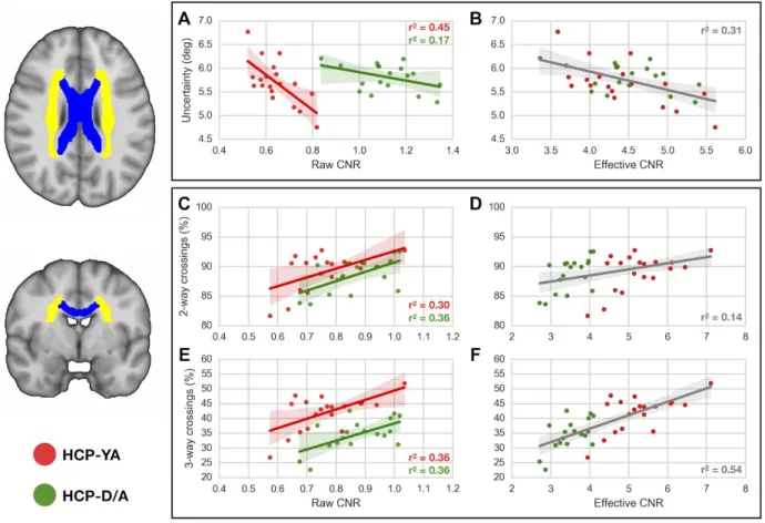
We compared the dMRI protocols for HCP-D/A and HCP-YA by quantifying their contrast-to-noise-ratio (CNR), uncertainty in estimating the main fiber orientation in the corpus callosum (CC), and their ability to estimate 2- and 3-way fiber crossings in the centrum semiovale (CSO). These particular measures were chosen because collectively they capture not only basic image quality (CNR) but also the impact of protocol choices such as voxel size and the specifics of the q-space sampling (e.g., number/distribution of shells) on some downstream measures derived during tractography. To investigate whether CNR is predictive of performance on the uncertainty and %-crossing measures we generated scatterplots of “Raw CNR” and “Effective CNR” versus those two measures (Figure 3; see caption for details). The HCP-D/A and HCP-YA protocols are similar in terms of fiber orientation uncertainty in the CC (Fig. 3A,B) and percentage of 2-way crossings detected in the CSO (Fig. 3C,D). However the percentage of 3-way crossings detected in the CSO is about 10 percentage points higher in the HCP-YA protocol compared to HCP-D/A (Fig. 3E,F), consistent with the increased total imaging time of the HCP-YA dMRI protocol. The scatterplots also indicate that Effective CNR is a reasonable single predictor of the uncertainty and %-crossing values across both protocols. The quantification in Figure 3 shows that the dMRI protocol for HCP-D/A has favorable properties relative to the dMRI protocol used for the HCP-YA study despite its 60% shorter overall acquisition duration. This sort of quantification is also valuable for situating the HCP-D/A and HCP-YA dMRI protocols in the context of other studies. Toward that goal, Supplemental Figure 3 contains a comparison of CNR that includes data from the UK Biobank project {Miller, 2016 #3200} (including quantification of CNR separately by b-value) and Supplemental Figure 4 is analogous to Figure 3, but with UK Biobank additionally included as part of the scatterplots.
Figure 3 (color). Comparison between HCP-D/A and HCP-YA dMRI protocols in terms of CNR, fiber orientation uncertainty, and detection of 2- and 3-way fiber crossings. For assessing the HCP-D/A protocol, we selected 18 older subjects from the Development (HCP-D) study, so that their mean age (18 years) would be reasonably close to the 19 selected HCP-YA subjects (mean age 28 years). “Raw CNR” was computed as part of FSL’s ‘eddy’ tool, which models and corrects for the effects of eddy currents and subject motion using a Gaussian Process (GP) model {Andersson, 2016 #3182}. For each subject, a CNR map was computed for each b-value shell as the ratio std(GP)/std(res) , where std(GP) is the standard deviation of the GP predictions from ‘eddy’ and std(res) is the standard deviation of the residuals (i.e., the difference between the observations and the GP predictions) for that b-value shell {Bastiani, 2018 #3433}. “Effective CNR” divides the raw (per image) CNR by the voxel volume, but multiplies it by the square root of the total number of volumes collected at a given b-value. Those normalizations reflect the presumption that CNR increases approximately linearly with voxel volume but by the square root of the number of (independent) samples when averaging. Two different analyses were run using two different ROIs in standard MNI space (left column): the corpus callosum (CC, blue) and the centrum semiovale (CSO, yellow). Uncertainty (expressed in degrees) in the estimation of the main fiber orientation in the CC was regressed onto the raw (A) and effective CNR (B) values (averaged across CC voxels and b-shells). Shaded area represents the 95% confidence region. For effective CNR we compute a single regression across the data from both protocols. The higher the CNR (i.e., higher angular contrast), the lower the uncertainty. Similarly, panels (C)-(F) show the dependency between raw and effective CNR values (averaged across CSO voxels and b-shells) and estimated sub-voxel fiber configuration complexity in the CSO, quantified as the percentage of voxels in the CSO mask where two
(C,D) or three (E,F) fiber populations were estimated. Up to three fiber compartments in each voxel were fitted using the multi-shell extension of the ball-and-stick model {Behrens, 2007 #2340;Jbabdi, 2012 #2928} using an automatic relevance determination prior weight of 1. Higher CNR results in the estimation of more crossing fibers, especially 3-way crossings.
3.4. Perfusion imaging
Arterial spin labeling (ASL) {Detre, 1992 #3356;Alsop, 2015 #3117} is a non-contrast-enhanced perfusion imaging method that provides quantitative measurements of cerebral blood flow (CBF) as a surrogate marker of brain metabolism and function, making it an informative complement to structural and functional connectivity measures. Cerebral blood flow is high during childhood and declines progressively during adolescence, stabilizing in later adolescence {Biagi, 2007 #3352}{Satterthwaite, 2014 #3375;Satterthwaite, 2014 #3375}. Age-associated alterations in vascular health are also important for understanding the basis of variation and disease in later life. Cerebral blood flow is a critical marker of neurovascular health that is altered across a range of conditions of aging including ‘typical’ aging {Chen, 2011 #3420;Zhang, 2017 #3421;Leenders, 1990 #3423;Parkes, 2004 #3424} and Alzheimer’s disease {Hays, 2016 #3467}. Despite recent progress, changes in CBF across the lifespan remain understudied. We accordingly included ASL in both the HCP-D and HCP-A imaging protocols to build foundational knowledge about this key aspect of brain function.
Although validated using 15O-water PET {Heijtel, 2014 #3364} and shown to be reproducible over time {Jain, 2012 #3368}, ASL imaging has a relatively low signal-to-noise ratio (SNR). Also, arterial transit time (ATT) -- the travel time of labeled blood from the labeling site to the imaged tissue -- is an essential parameter in CBF quantification, yet it changes during normal development and aging {Hutchins, 1996 #3367}. Thus, it is important to simultaneously measure ATT and CBF by performing ASL imaging acquisition with multiple post-labeling delays. We also strove to maximize spatial resolution for ASL to improve the ability to assess subtle perfusion changes in the cortical gray matter ribbon and in small subcortical brain regions.
Improving ASL resolution is challenging, especially for a multi-delay protocol and within the ~5 min acquisition time available in our overall protocol. Recently, several studies have reported improvements in the SNR efficiency of ASL. Pseudo-continuous arterial spin labeling (PCASL) can improve labeling efficiency and perfusion SNR {Wu, 2007 #2249;Dai, 2008 #3354}. Single-shot 3D imaging methods, such as 3D GRASE {Gunther, 2005 #3363}, have been applied for PCASL imaging to increase perfusion SNR, with segmented 3D imaging readouts used to reduce spatial blurring due to T 2 decay {Tan, 2011 #3376}. Segmented 3D PCASL has been recommended as a consensus choice for ASL in clinical applications {Alsop, 2015 #3117}. However, segmented 3D acquisitions to improve spatial resolution are highly sensitive to head motion common in young children and elderly subjects. Recently, multiband (MB)/simultaneous multislice (SMS) 2D EPI has been successfully applied for high resolution whole brain PCASL imaging with a demonstrated improvement in perfusion SNR efficiency {Li, 2015 #3116}. Compared to segmented 3D GRASE, 2D MB-EPI is less sensitive to subject motion due to its accelerated single-shot volume acquisition.
For HCP-D/A we evaluated two acquisition strategies for multi-delay PCASL imaging: single-shot 2D MB-EPI and segmented 3D GRASE with background suppression. The total acquisition time was limited to approximately 5 minutes for five post-labeling delays. An initial pilot study using low spatial resolution (3.5 mm isotropic voxels) and healthy young adults showed no significant differences between the 2D and 3D approaches on ATT and CBF quantified in 6 subjects (Figure 4) {Li, 2017 #3371}, indicating consistent quantification with either approach. However, significant T 2 blurring was present in 3D GRASE (collected with 4 segments) and 2D MB-EPI was less sensitive to subject motion, and thus suffered less from data loss compared to 3D GRASE. Compared to 2D MB-EPI, 3D GRASE acquires fewer perfusion measurements within the same scan duration, as the acquisition time per volume is longer due to the segmented acquisition. In particular, only a single measurement could be acquired for three of the post-labeling delays for the piloted multi-delay 3D GRASE protocol, thus potentially compromising ATT measurement if even just a single volume was corrupted due to motion, which is likely to be a common problem in the young and elderly populations of the HCP-D/A projects. Together these factors motivated us to choose 2D MB-EPI over 3D GRASE for multi-delay PCASL imaging.
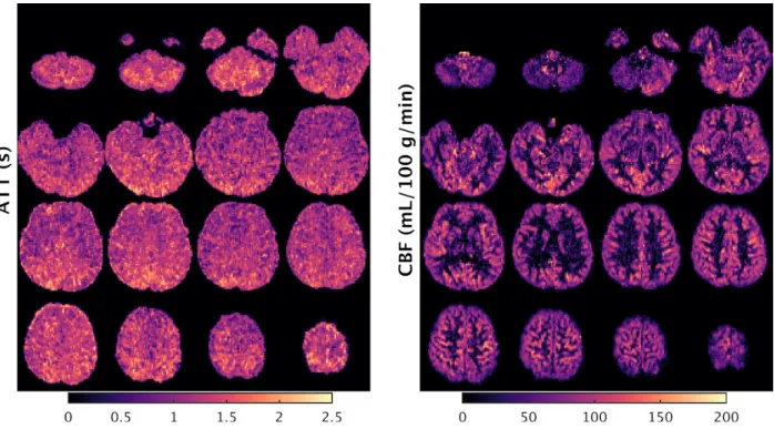
A second pilot study evaluated high spatial resolution PCASL scans (2.5 mm isotropic), closer to that of the other imaging modalities (and to our recommendations for ‘HCP-style’ paradigms) {Glasser, 2016 #3197}. Due to the prevalence of motion issues using 3D GRASE, this pilot study focused on 2D MB-EPI PCASL. Figure 5 shows ATT and CBF maps acquired using the high-resolution 2D MB-EPI protocol for one subject. This high-resolution multi-delay 2D MB-EPI PCASL protocol yielded high quality ATT and CBF maps, and provided plausible ATT and CBF estimates (Figure 4), thereby warranting its adoption for CBF quantification in both HCP-D and HCP-A.
Figure 4. Measurements of arterial transit time (ATT) and cerebral blood flow (CBF) in gray (GM) and white (WM) matter from the multi-delay PCASL pilot studies. A ‘low’ spatial resolution pilot study collected 3D GRASE (collected with four segments, in black) and 2D MB-EPI with an MB factor of 6 (in dark gray) in the same subjects (N=6, 3M/3F, mean age of 28 years), with 3.5 mm voxels over 4.5
minutes. A ‘high’ spatial resolution resolution pilot collected 2D MB-EPI with an MB factor of 6 and 2.5 mm voxels over 5.5 minutes (in light gray) in a different set of subjects (N=5, 2M/3F, mean age of 28 years). The error bars represent the standard deviations. For the low spatial resolution (3.5 mm) pilot, no significant differences were found between the ATT or CBF values in either GM or WM between the 2D and 3D approaches (paired t-test), indicating comparable ATT and CBF quantification with either approach {Li, 2017 #3371}. There were also no significant differences between the ATT or CBF values in either GM or WM between the low and high spatial resolution 2D MB-EPI acquisitions (t-test). Preprocessing of the ASL data for the ATT and CBF quantification was performed using SPM (i.e., GM/WM segmentation of a T1w anatomical scan, and motion correction and coregistration). ATT maps were generated based on the weighted delay approach {Dai, 2012 #3447}, and CBF maps generated using a single compartment perfusion model that took into account the estimated ATT {Wang, 2013 #3448} using custom Matlab scripts. Mean ATT and CBF within GM and WM was then computed for each subject.
Figure 5 (color). High spatial resolution 2D MB-EPI PCASL. An example subject’s (male, 21 years old) arterial transit time (ATT) and cerebral blood flow (CBF) maps acquired using 2D MB-EPI PCASL with high spatial resolution (2.5 mm in-plane resolution with sixty 2.27 mm thick slices with a 10% slice gap) and five post-labeling delays (0.2, 0.7, 1.2, 1.7 and 2.2 s) with a 5.5 minute overall duration. The axial slices displayed are spaced by 7.5 mm, with the left hemisphere of the brain on the left side of the image. See Figure 4 caption for details regarding the generation of the ATT and CBF maps.
During the ASL scan, participants 8 years and older view a small white fixation crosshair on a black background (same as for the rfMRI scans). However, the 5-7 year olds in HCP-D are allowed to watch a movie during the ASL scan, given concerns about asking the youngest children to view a fixation cross for 5.5 minutes. We avoid having the older children and adults