R E S E A R C H A R T I C L E
Open Access
A computational framework for
complex disease stratification from
multiple large-scale datasets
Bertrand De Meulder
1*†, Diane Lefaudeux
1†, Aruna T. Bansal
2, Alexander Mazein
1, Amphun Chaiboonchoe
1,
Hassan Ahmed
1, Irina Balaur
1, Mansoor Saqi
1, Johann Pellet
1, Stéphane Ballereau
1, Nathanaël Lemonnier
1, Kai Sun
3,
Ioannis Pandis
3,4, Xian Yang
3, Manohara Batuwitage
3, Kosmas Kretsos
5, Jonathan van Eyll
6, Alun Bedding
7,
Timothy Davison
4, Paul Dodson
8, Christopher Larminie
9, Anthony Postle
10, Julie Corfield
11,12, Ratko Djukanovic
10,
Kian Fan Chung
13, Ian M. Adcock
13, Yi-Ke Guo
3, Peter J. Sterk
14, Alexander Manta
15, Anthony Rowe
4, Frédéric Baribaud
16,
Charles Auffray
1*and the U-BIOPRED Study Group and the eTRIKS Consortium
Abstract
Background:
Multilevel data integration is becoming a major area of research in systems biology. Within this area,
multi-
‘
omics datasets on complex diseases are becoming more readily available and there is a need to set standards
and good practices for integrated analysis of biological, clinical and environmental data. We present a framework to
plan and generate single and multi-
‘
omics signatures of disease states.
Methods:
The framework is divided into four major steps: dataset subsetting, feature filtering,
‘
omics-based clustering
and biomarker identification.
Results:
We illustrate the usefulness of this framework by identifying potential patient clusters based on integrated
multi-
‘
omics signatures in a publicly available ovarian cystadenocarcinoma dataset. The analysis generated a higher
number of stable and clinically relevant clusters than previously reported, and enabled the generation of predictive
models of patient outcomes.
Conclusions:
This framework will help health researchers plan and perform multi-
‘
omics big data analyses to generate
hypotheses and make sense of their rich, diverse and ever growing datasets, to enable implementation of translational
P4 medicine.
Keywords:
Molecular signatures,
‘
Omics data, Stratification, Systems medicine
Background
Since the early days of medicine, practitioners have
always combined their observations from patient
exami-nations with their medical knowledge and experience to
diagnose medical conditions and find treatments tailored
to the patient [
1
]. Nowadays, this rationale includes the
integration of molecular, clinical, imaging information
and other data sources to inform diagnosis and
progno-sis [
2
] or in other words, personalised medicine.
Various data integration methods developed through
systems biology and computer science are now available
to researchers. These methods aim at bridging the gap
between the vast amounts of data generated in an
ever-cheaper way [
3
] and our understanding of biology
reflecting the complexity of biological systems [
4
].
Promises of data integration are the reduced cost of
clin-ical trials, better statistclin-ical power, more accurate
hypoth-esis
generation
and
ultimately,
individualised
and
cheaper healthcare [
2
].
However, a lack of communication exists between the
fields of clinical medicine and systems biology,
bioinfor-matics and biostatistics, as suggested by the reluctance
* Correspondence:[email protected];[email protected]†Bertrand De Meulder and Diane Lefaudeux contributed equally to this work.
1European Institute for Systems Biology and Medicine, CNRS-ENS-UCBL, EISBM, 50 Avenue Tony Garnier, 69007 Lyon, France
Full list of author information is available at the end of the article
© The Author(s). 2018Open AccessThis article is distributed under the terms of the Creative Commons Attribution 4.0
International License (http://creativecommons.org/licenses/by/4.0/), which permits unrestricted use, distribution, and reproduction in any medium, provided you give appropriate credit to the original author(s) and the source, provide a link to the Creative Commons license, and indicate if changes were made. The Creative Commons Public Domain Dedication waiver (http://creativecommons.org/publicdomain/zero/1.0/) applies to the data made available in this article, unless otherwise stated.
or distrust to recent developments of personalised
medi-cine by the medical community [
1
,
5
,
6
]. To address this
issue, we developed a computational/analysis framework
that aims at facilitating communication between
health-care
professionals,
computational
biologists
and
bioinformaticians.
Among several ways of integrating data across
bio-logical levels, one of the components is multi-omics data
integration. The identification of molecular signatures
has been a focus of the biology and bioinformatics
com-munities for over three decades. Early studies focused on
a small number of molecules, paving the way for larger
studies, eventually supporting the emergence of the
‘omics’
concept in the late 1990’s, starting with
‘genom-ics’
[
7
,
8
]. Owing to both technical and biological
ad-vances, many classes of molecules have been studied by
‘omics technologies such as transcriptomics [
9
–
11
],
pro-teomics [
12
,
13
], lipidomics [
14
,
15
], metabolomics (first
mentioned in [
16
,
17
]), the composition of the exhaled
breath by breathomics (first mentioned in [
18
]) [
19
], and
interactomics [
20
,
21
], among others.
Consequently, bioinformatics tools have been
devel-oped to analyse this new wealth of biological data, as
reviewed in [
22
]. The concept of systems biology was
de-veloped first in the 1960’s [
23
,
24
] to study biological
or-ganisms as complete and complex systems, integrating
various sources of information (phenotypic data,
mo-lecular data, etc.) in combination with pathway/network
analysis and mathematical modelling [
25
–
33
]. These
sys-tems approaches are highly suitable for the discovery of
disease phenotypes (based on empirical recognition of
observed characteristics) and so-called endotypes
(cap-turing complex causative mechanisms in disease) [
34
].
The logical next step was to apply systems biology tools
to improve clinical diagnosis, refine the endotypes
lead-ing to diseases, develop a comprehensive approach to
the human body and assess an individual’s health in light
of its
‘omics status. In this way the
‘systems medicine’
concept was born [
35
–
41
]. The systems medicine
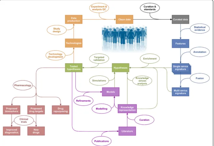
ration-ale is outlined in Fig.
1
.
Any meaningful experiment relies on a robust,
bias-controlled study design [
42
] using appropriate
technolo-gies, leading to the production of trustworthy
quality-checked data. Data curation then aims at organising,
annotating, integrating and preserving data from various
sources for reuse and further integration. The next step is
to identify relevant molecular features using statistical
evidence. A tremendous and constantly growing number
of methods is available for this purpose, making the
process of method selection a crucial and challenging task.
We provide some guidelines here but recommend that
the reader turns to specialised reviews (such as [
43
]) for
more insights on the relevance and appropriateness of
in-dividual methods. Once features are statistically selected,
their annotation is required to interpret results and
pro-duce a single
‘omic signature. Annotation is a complex
task that links identifiers from the technological platforms
to existing entities (i.e. genes, peptides, metabolites, lipids,
etc.) [
44
,
45
]. If the data permit, information from several
‘omics platforms is integrated into multi-‘omics signatures.
Single and multi
‘omics signatures ultimately serve to
identify molecular mechanisms driving pathobiology.
Contextualisation of signatures with existing
know-ledge is now standard practice (e.g. ontology, enrichment
and pathway analysis [
46
]), or performed with more
ad-vanced tools for data integration and visualisation such
as a disease map [
47
]. Exploratory analysis using
network-based information is valuable, with tools such
as the STRING database [
48
], among many others.
Hy-potheses can then be formulated and tested in two ways,
with external datasets and/or new experiments; or by
modelling and knowledge representation (see review in
[
49
] and disease maps examples in [
47
,
50
–
52
]). With
the help of systems pharmacology (see [
53
]), outcomes
of this whole exercise are enabling: (i) identification of
new potential drug targets associated with newly
identi-fied patient clusters, (ii) elucidation of potential
bio-markers for diagnosis, (iii) repurposing of existing drugs
and, ultimately, (iv) changes in diagnostic processes and
development of new drugs and treatments for disease
management. The key step in the systems medicine
process is pattern recognition, for which a robust and
step-wise framework is required.
Definitions
Our article focuses on the identification of disease
mechanisms through statistical analysis of raw data,
an-notation with up-to-date ontologies to generate
finger-prints
(biomarker signatures derived from data collected
from a single technical platform),
handprints
(biomarker
signatures derived from data collected within multiple
technical platforms, either by fusion of multiple
finger-prints or by direct integration of several data types) and
interpretation on a pathway level to identify
disease-driving mechanisms.
One way to better define the different endotypes is to
generate molecular fingerprints (e.g. blood cell
tran-scriptomics analysis yields genes differentially expressed
between clinical populations [
54
]) and handprints (e.g.
mRNA expression, DNA methylation and miRNA
expres-sion data fused to generate clusters of cancer patients
[
55
]). The latter can be combined to study patients e.g. at
the
‘blood biological compartment’
level, and linked with
specific disease markers to better define the underlying
biology, hence providing new avenues for therapy.
Despite the wealth of
‘omics analyses, little consensus
exist on which statistical or bioinformatics methods to
apply on each type of data set, nor on the
‘best’
integrative
methods for their combined analysis (although standards
exist for some data types, see [
22
]). Here, we present a
gen-eric framework to perform statistical and bioinformatics
ana-lyses of
‘omics measurements, starting from raw data
management to multi-platform data integration, pathway and
network modelling that has been adopted by the Innovative
Medicines Initiative (IMI) U-BIOPRED Consortium
(Un-biased BIOmarkers for the PREDiction of respiratory disease
outcomes,
http://www.ubiopred.eu
) and extended in the
eTRIKS Consortium (
https://www.etriks.org/
) to support a
large number of national and European translational
medi-cine projects. This article is not a review of the very large
body of literature on relevant bioinformatics methods.
In-stead it describes generic steps in
‘omics data analysis to
which many methods can be mapped to help
multidisciplin-ary teams comprising clinical experts, wet-lab researchers,
bioinformaticians, biostatisticians and computational systems
biologists share a common understanding and communicate
effectively throughout the systems medicine process [
56
].
We illustrate our pragmatic approach to the design
and implementation of the analysis pipeline through a
handprint analysis using the TCGA Research Network
(The Cancer Genome Atlas
–
http://cancergenome.nih.
gov
/) Ovarian serous cystadenocarcinoma (OV) dataset.
Data preparation: Quality control, correction for
possible batch effects, missing data handling, and
outlier detection
Quality Control (QC) comprises several important steps
in data preparation. First, the platform-specific technical
QC and normalisation are performed according to the
standards of the respective fields of each particular
technological platform.
Batch effects are a technical bias arising during study
design and data production, due to variability in
produc-tion platforms, staff, batches, reagent lots, etc. Their
im-pact can be assessed using descriptive methods such as
Principal Component Analysis (PCA) and graphical
dis-plays. Tools such as ComBat [
57
] and methodologies
de-veloped by van der Kloet [
58
] can be used to adjust for
batch effects when necessary.
Fig. 1Outline of the Systems Medicine rationale. Represented in orange are the steps linked to quality data production, followed by curation in grey, identification of interesting features through statistical analysis in blue and hypothesis generation and their validation in green. Modelling and knowledge representation methods can inform the hypotheses generated through statistical analysis of generated hypotheses on their own (in purple). Outputs of this exercise are represented in red: drug repurposing, new drugs and improved diagnostics, with the help of clinical trials
Missing data are features of all biological studies and
arise for a variety of reasons. If the source of the
miss-ingness is unrelated to phenotype or biology, the missing
data points can be classified as Missing Completely At
Random (MCAR). Such missing values may be handled
through imputation (to the mean, mode, mean of
near-est neighbours, or by multiple imputation etc.) or by
simple deletion [
59
].
Additional non-random missing data may arise due to
assay- or platform-specific performances. For example,
the measurement of abundances can fall below the lower
limit of detection or quantitation (LLQ) of the
instru-ment. In such instances, imputation is generally applied.
Common methods include imputation to zero, LLQ,
LLQ/2, or LLQ/
√
2; extrapolation and maximum
likeli-hood estimation (MLE) can also be used [
59
].
Particular difficulty occurs in the analysis of mass
spectrometry data, when it is impossible to distinguish
MCAR data points from those below the LLQ of the
technique. The combined levels of missing data often far
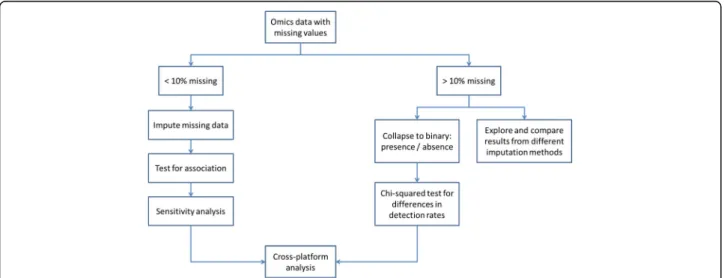
exceed 10%. For these, the process depicted in the Fig.
2
is proposed.
Critical appraisal of the pattern of missingness is
cru-cial. Where extensive imputation is applied, the
robust-ness of imputation needs to be assessed by re-analysis,
using a second imputation method, or by discarding the
imputed values.
Outliers are expected in any biological/platform data.
When these are clearly seen to arise due to technical
ar-tefacts (differences by many orders of magnitude, etc.),
they should be discarded. Otherwise and in general,
out-lying values in biological data should be retained, flagged
and subjected to statistical analysis.
When there is no community-wide consensus on a
specific quality threshold for a particular biological data
type, the research group generating the data applies
quality filters on the basis of their knowledge and
experi-ence. Precise description of each data processing step
should accompany each dataset to inform colleagues
performing downstream analysis.
Methods
The framework concept
Several key generic steps in data analysis were identified
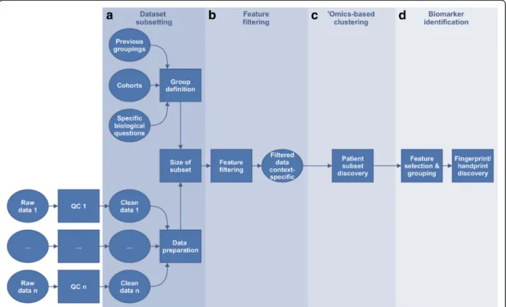
and are highlighted in Fig.
3
below.
Step 1: Dataset subsetting
This first box of Fig.
3
3 comprises two major steps: 1)
formulating the biological question to be addressed and
2) preparing the data.
Formulating the biological question
Several types of biological questions can be tackled,
leading to different partitions of the dataset(s) to study.
A partitioning scheme may rely on cohort definitions
based on current state of the art, a specific biological
question (e.g. comparing highly atopic to non-atopic
severe asthmatics), or clustering results, obtained with
clinical variables alone, distinct specific
‘omic or
multi-‘omics clustering, etc.
Data preparation
Depending on the question formulated at the previous
step, data are then subsetted when appropriate. Then, an
additional outlier detection check, data transformation
and normalisation step can be performed, with methods
Fig. 2Process proposed for handling high levels of non-random missing data. If there are less than 10% missing values, data imputation is used, then tested for association (artificial associations might arise from the imputation process, which would then skew the analysis downstream) and submitted to a sensitivity analysis. If there are more than 10% missing values, we either collapse the feature/patient to a binary (presence/absence) scheme and run aχ2test for difference in detection rates, or explore several imputation methods with highly cautious interpretation
described above. In this step, the statistical power that
the analyst can expect (or the effect size that can be
ex-pected to be discovered) can be investigated (for more
details on the computation of statistical power in
‘omics
data analysis, see [
60
]). A decision on whether to split
the datasets into training and validation sets is also made
at this point (see section 4, replication of findings).
Step 2: Feature filtering
Given the complexity and large amount of clinical and
‘omics data in a complex dataset, the number of features
measured is vastly superior to the number of replicates
creating various statistical challenges, i.e.. the
‘curse of
dimensionality’
[
61
,
62
]. Feature filtering (Fig.
3b
) is
therefore often used to select a subset of features
rele-vant to the biological question studied, remove noise
from the dataset and reduce the computing power and
time needed [
63
–
65
].
Features can be filtered according to specific criteria,
based for example on nominal
p
-values arising from
com-parison between groups. Indeed, several methods exist to
perform feature filtering, based on mean expression
values, p-values, fold changes, correlation values [
66
,
67
],
information content measures [
68
,
69
], network-based
metrics (connectivity, centrality [
70
,
71
]) or using a
non-linear machine learning algorithm [
72
]. We
redir-ect the reader to the following reviews for more details
[
33
,
73
–
75
]. As this step might introduce bias into the
downstream analyses, it is not always applied.
Step 3:
‘
Omics-based clustering
Clustering analysis groups elements so that objects in the
same group are more similar to each other than to those
in other groups (Fig.
3c
). All methods available rely on
similarity or distance measures and a clustering algorithm
[
76
–
78
]. The most classical clustering methods may be
categorized as
‘partitioning’
(constructing
k
clusters) or
‘hierarchical’
(seeking to build a hierarchy of clusters), and
either agglomerative (each observation starts in its own
cluster, and pairs of clusters are merged as one moves up
the hierarchy, ending in a single cluster) or divisive (all
ob-servations start in the same cluster and splits are
per-formed recursively as one moves down the hierarchy,
ending with clusters containing one single observation).
It is important to note that clustering techniques are
descriptive in nature and will yield clusters, whether they
Fig. 3Overview of the framework. Starting from quality-checked and pre-processed‘omics data, four key generic steps are highlighted: (a) dataset subsetting, including formulation of the biological question to be answered and data preparation, (b) feature filtering (optional step) where features that are uninformative in relation to the question can be removed, (c)‘omics-based unsupervised clustering (optional step) aiming at finding groups of participants arising from the data structure using the (optionally filtered) features, and finallyd) biomarker identification, including feature selection by bioinformatics means and machine learning algorithms for prediction
represent reality or not [
76
]. One way of finding out
whether clusters represent reality is to assess their
stabil-ity, with the consensus clustering approach [
79
] for
example. Using different stable clustering algorithms on
the same dataset and comparing them with the
meta-clustering rationale [
80
] is a further step to assess if
clus-ters represent accurately and reproducibly the biological
situation in the data.
When several
‘omics datasets on the same patients are
available, a handprint analysis can be performed with the
Similarity Network Fusion (SNF) method to derive a
patient-wise multi-‘omics similarity matrix [
55
]. Other
methods for data integration in the context of subtype
dis-covery are available such as iCluster [
81
], Multiple Dataset
Integration [
82
], or Patient-Specific Data Fusion [
83
], further
discussed in [
84
] or under development, for example by the
European Stategra FP7 project (
http://www.stategra.eu
).
Step 4: Biomarker identification
Steps 1 to 3 aim at finding groups of patients to best
describe the biological condition(s), with respect to the
questions addressed. Step 4 aims at 1) finding the
smallest set of molecular features whose difference in
abundance between these patient groups (Fig.
3d
) enable
their distinction (biomarkers) and 2) building
classifica-tion models through machine-learning techniques, some
of which use both feature reduction and classification
model building together. The outcome is a fingerprint or
handprint, depending on the number of different
‘omics
datasets included in the analysis.
Over-fitting and false-discovery rate control
As already mentioned,
‘omics technologies suffer from
what is known as the
‘curse of dimensionality’
, typically
due to the large number of features (p) and low number
of samples (n). As statistical methods were historically
developed for a situation where the dimensions were n
>> > p instead of the p >> > n situation, methods
adjust-ments had to be made. The main issue in statistical
analysis is the high type I error rate (false positives) in
null hypothesis testing. Several ways of correcting for
this have been developed, the most well-known and used
being the Bonferroni correction and the
Benjamini-Hochberg False Discovery Rate (FDR) controlling
procedure [
85
]. Discussions are still ongoing in the
sta-tistics community as to which method is best to control
the false positive rates in the context of
‘omics data
analysis [
46
,
86
,
87
]. We therefore advise to split the
data in testing and validation groups. Tests made
within each group are corrected for FDR with the
Benjamini-Hochberg’s procedure whenever possible or
advised by domain experts, and only features detected
in both groups should be considered for further
ana-lysis and interpretation.
Over-fitting may occur when a statistical model
includes too many parameters relative to the number of
observations. The over-fitted model describes random
error instead of the underlying relationship of interest
and performs poorly with independent data. In deriving
prediction models therefore, a guiding principle is that
there should be at least ten observations (or events) per
predictor element [
88
] while simple models with few
parameters should be favoured whenever possible.
All in all, the combination of internal replication, FDR
correction and conservative over-fitting considerations
allows the detection of interesting
‘omics features with a
reference statistical foundation.
Replication of findings
When a large number of statistical tests have been
planned, a comprehensive adjustment for multiple
test-ing can be detrimental to statistical power. Validation
and replication of findings is therefore essential in order
to avoid the widespread unvalidated biomarker
syn-drome that has plagued the vast majority of claimed
bio-markers. Indeed, fewer than 1/1000 have proved
clinically useful and approved by regulatory authorities
[
89
–
94
]. For each combination of platform and sample
type, an assessment can be made as to whether the data
should be split into training and validation sets, or
instead analysed as a single pool.
The predictive value of a biomarker identified after
proper internal replication applies to the dataset in
which it was discovered. Replication of findings in
add-itional sample sets is a crucial step in producing
clinic-ally usable biomarkers and predictive models [
95
,
96
]
and should thus always be sought.
Once the feature filtering step is performed, the next
step is to make sense of the results, either in a biological
or mathematical manner. Biological annotation can be
performed using pathways (see review in [
97
]) or
func-tional categories (reviewed in [
98
]); however, this kind of
analysis is hampered by factors such as statistical
consid-erations (which method to use, independence between
genes and between pathways, how to take into account
the magnitude of the changes) and pathway architecture
considerations (pathways can cross and overlap, meaning
that if one pathway is truly affected, one may observe
other pathways being significantly affected due to the set
of overlapping genes and proteins involved) [
99
]. One
way of overcoming those limitations is to use the
complete genome-scale network of protein-protein
inter-actions to define affected sub-regions of the network,
with available academic [
100
,
101
] and commercial
solu-tions (e.g. MetaCore™
Thomson Reuters, IPA Ingenuity
Pathway Analysis). A recent proposed solution is the
dis-ease map concept, following the examples of the
Parkin-son’s disease map [
47
], the Atlas of Cancer Signalling
Networks [
50
] and the AlzPathway [
51
,
52
] where an
ex-haustive set of relevant interactions to a particular
dis-ease are represented in details as a single network,
which can then be analysed biologically and
mathematic-ally, with the supervision of domain experts for coverage
and specificity [
102
].
Results
Application to a public domain dataset: TCGA OV dataset
for handprint analysis
The Cancer Genome Atlas (TCGA,
http://cancergenome.
nih.gov
/) is a joint effort of the National Cancer Institute
(NCI) and the National Human Genome Research
Insti-tute (NHGRI) in the USA. It aims to accelerate our
under-standing of the molecular basis of cancer through
application of genome analysis technologies. Among other
functionalities, TCGA offers a freely available database of
multi-‘omics datasets (including clinical data, imaging,
DNA, mRNA and miRNA sequencing, protein, gene exon
and miRNA expression, DNA methylation and copy
num-ber variation (CNV)) for several cancer types, with patient
numbers ranging from a few dozens to above a thousand.
As a use case, the ovarian cancer OV dataset was
chosen, as it comprises several
‘omics measurements for a
large group of patients; this dataset has already been well
characterized in several publications but without a data
fu-sion analysis, in contrast to the glioblastoma TCGA
data-set, for example [
55
]. It comprises data from a total of 586
patients, along with several
‘omics datasets (such as SNP,
Exome, methylation…), as shown in the Table
1
.
below.
All data matrices were downloaded using the Broad
Insti-tute FireBrowse TCGA interface (
http://firebrowse.org/
?cohort=OV&download_dialog=true
#); the results shown
here are based upon data generated by the TCGA
Re-search Network.
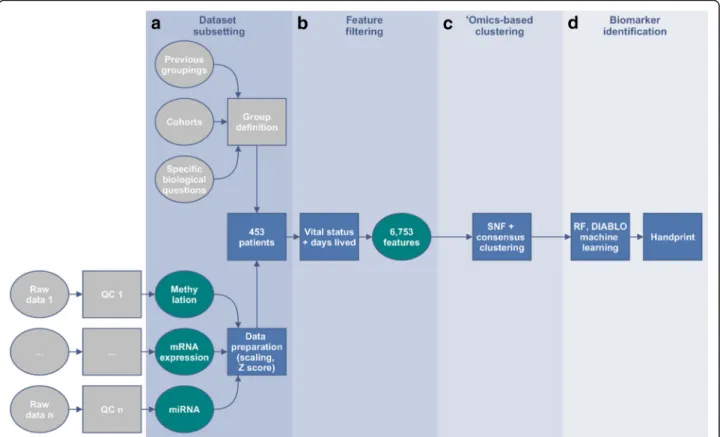
Data preparation
We used the clinical, methylation, mRNA and miRNA
data matrices from the 453 patients (out of a total of
586 patients) for which all four data types were available.
The overview of the analysis is summarized in the Fig.
4
.
Feature selection
Preliminary analysis without feature selection was
per-formed (data not shown). Briefly, this analysis led to the
identification of four stable clusters, mainly differentiated
by lymphatic and venous invasion status and clinical stage.
Biologically speaking, the comparison of clusters led to
the highlighting of well-known ovarian cancer biomarkers
and pathways.
In order to produce a handprint more focused on the
survival status of patients in the dataset, each
‘omics
dataset was treated separately to identify features
associ-ated with survival status at the end of the study and
overall survival time. The latter was obtained by
sum-ming the age (in days) of the participants at enrolment
in the study and the post-study survival time, both
values available in the clinical variables from the TCGA
website. After data preparation including imputation of
missing data in methylation and normalisation, linear
models testing for survival status with survival time as a
cofactor were fitted feature-wise and
p
-values for
differ-ential expression/abundance were derived. All features
with a nominal p-value < 0.05 were selected. This yielded
a total of 899 features in the methylation dataset, 37
miRNAs and 5817 probesets in transcriptomics.
‘
Omics-based clustering
Similarity matrices were derived from each filtered
‘omics dataset, which were fused with SNF, and spectral
clustering with a consensus clustering step was applied
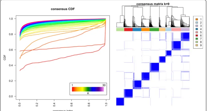
to detect stable clusters, as shown in Fig.
5
below. The
choice of the optimal number of stable clusters is based
on two mathematical parameters: the deviation from
ideal stability (DIS, a measure of the deviation from
horizontality of the CDF curves in the left panel of the
Fig.
5
, the formulation of which can be found in the
supplementary material of [
103
]), and the number of
pa-tients assigned in each cluster (clusters with fewer than
10 patients should be avoided [
58
]). The DIS across the
number of clusters can be found in the Additional file
1
.
The DIS shows a minimal value for k = 3 clusters, but
very similar values can be seen for k = 6, 7, 9, 10, 11 and
12. As it is clinically interesting to distinguish a higher
number of clusters and to define clusters with different
survival status, we chose the number of clusters
associ-ated with low DIS, no clusters with fewer than 10
pa-tients, and statistically significant differences in survival
status and survival time of patients, k = 9.
The clinical characteristics of the nine clusters are
shown in Table
2
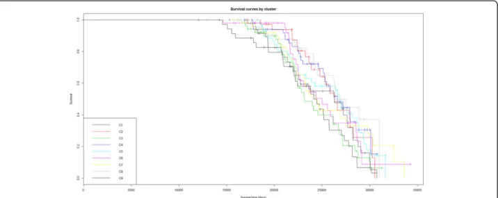
. Survival curves are also shown in
the Kaplan-Meyer plot (Fig.
6
). Survival status and
survival time differ between the nine clusters,
show-ing for example that patients in cluster 1 have a
higher mortality rate.
Table 1
This table shows the number of cases in each
‘
omics platform available for the TCGA Ovarian Serous Cystadenocarcinoma
dataset (source:
https://gdc.cancer.gov/
)
Ovarian serous cystadenocarcinoma Total Exome SNP Methylation mRNA miRNA Clinical
Biomarker identification
Enrichment analysis
In order to detect differentially expressed features that are
specific to one group, each of the nine clusters was
com-pared to the rest of the dataset. Table
3
shows the
sum-mary of statistically different features (
p
-value < 0.05, 5%
FDR correction) identified in each comparison.
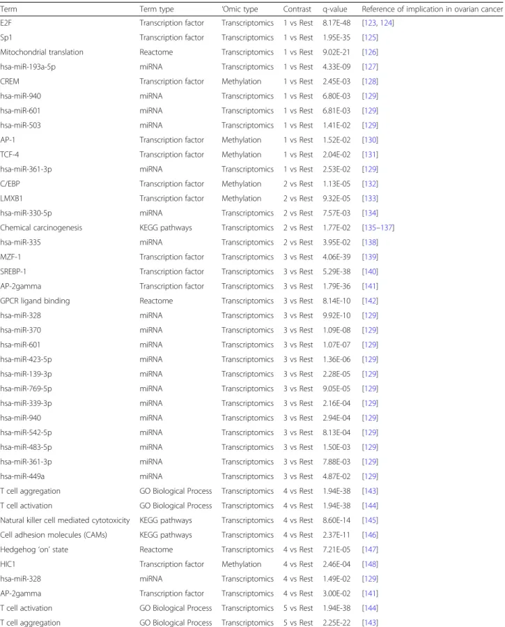
Enrichment analysis of features differentially expressed/
abundant between the clusters was then performed.
Complete results are presented in the Additional file
2
; an
overview of results for which there is already evidence in
the literature is presented below in Table
4
.
In short, the biological functions enriched in each
cluster are as follows: cluster 1 is mostly enriched in
mitochondrial translation and energy metabolism, cell
cycle regulation, negative regulation of apoptosis and
DNA damage response. In addition, several miRNAs and
transcription factors are enriched; the details can be
found in the Additional file
2
.
Cluster 2 is associated with chemical carcinogenesis,
miR-330-5p, miR-693-5p and the Pax-2 transcription
factor. Other transcription factors are also highlighted
through the methylation measurements.
Cluster 3 is associated with immune system regulation (T
cell-related processes, and more precisely CD4 and CD8-T
cells lineages-related processes…), cell-cell signalling,
cAMP signalling, cytokine-cytokine interaction, G-Protein
coupled receptor (GPCR) ligand binding and neuronal and
muscle-related pathways (potassium and calcium channels,
other ion channels and synapses). Again, several miRNAs
and transcription factors are highlighted.
Cluster 4 is also associated with the immune response,
and key functions such as lymphocyte activation, T cell
aggregation, differentiation, proliferation and activation,
adaptive immune system, regulation of lymphocyte
cell-cell activation, immune response-regulating signalling
pathway, cytokine-cytokine receptor interaction, antigen
processing and presentation, hematopoietic cell lineage
and hematopoiesis and B cell activation. Primary
im-munodeficiency pathway and cell adhesion molecules,
along with miR-938 and several transcription factors are
also enriched.
Fig. 4Framework outline for the TCGA handprint analysis with additional feature filtering. Each dataset was separately filtered based on nominal
p-values < 0.05 when comparing alive versus deceased patients at the end of the study taking into account the total amount of days alive. A total of 6753 features were selected: 899 differentially methylated genes, 37 miRNAs and 5817 differentially expressed probesets. Consensus clustering on the fused similarity matrices determined the number of stable clusters that were viewed in a Kaplan-Meyer plot and tested for differential survival. Machine learning was then performed to identify candidate features predicting the identified groups: Recursive Feature Elimination (RFE) on a linear Support-Vector-Machine (SVM) model to identify informative features, followed by a Random Forest (RF) model building in parallel with DIABLO sPLS-DA on those features
Cluster 5 is related to immune response, enriched in
lymphocyte activation, T cell aggregation, differentiation,
activation and proliferation, leukocyte differentiation,
ag-gregation and activation, positive regulation of cell-cell
adhesion, antigen processing and presentation, cytokine
production, inflammatory response, NK cell-mediated
cytotoxicity and cytokine-cytokine receptor interaction.
Other processes involved are NF-
κ
B signalling,
Jak-STAT signalling, Interferon
α
/
β
signalling, TCR
signal-ling, VEGF signalsignal-ling, VEGFR2-mediated cell
prolifera-tion, Hedgehog
‘off
’
state, along with several miRNAs
and transcription factors.
Cluster 6 is enriched in several signalling pathways,
such as cAMP, GPCR signalling, arachidonic acid
metab-olism and fatty acids metabmetab-olism, as well as positive T
cell selection, several miRNAs and transcription factors.
Cluster 7 is linked with respiratory metabolism, p53
and cell cycle regulation, splicing regulation as well as
signalling by NF-
κ
B and miRNAs and transcription
factors.
Cluster 8 is enriched with T cell lineage
commit-ment, potassium channels, miRNAs and transcription
factors.
Cluster 9 is associated with ion transport (including
syn-aptic, calcium and potassium channels), cAMP signalling,
nicotine addiction, as well as miRNAs and transcription
factors.
Each cluster is linked with one or several of the
well-known hallmarks of cancer such as regulation of the cell
cycle (clusters 1 and 7), energy metabolism (cluster 1 and 7),
immune system (clusters 3, 4, 5 and 8),
epithelial-to-mesenchymal transition (cluster 4) or angiogenesis
(cluster 5) [
104
–
106
]. Interestingly, our analysis based
on
‘omics profiles is able to identify clusters that seem to
separate some of those hallmarks out, while an analysis
taking into account only the clinical data cannot. As seen
above, cluster 6 is associated with a higher rate of survival.
It would therefore be interesting to further explore the
signalling networks enriched in the comparison between
cluster 6 and the other clusters to identify the molecular
mechanisms responsible for the extended survival.
Machine-learning predictive modelling
The next step in the analysis is to establish a model that
can predict which cluster a patient belongs to, based on
the
‘omics measurements alone. Machine-learning
tech-niques (reviewed in [
107
,
108
]), available in the caret R
package [
109
] and in the MixOmics R packages [
110
,
111
] were used.
Two models were built in parallel, on the same dataset.
1. A Recursive Feature Elimination (RFE) procedure
was performed to identify the smallest number of
features from the three
‘omics platforms that allow
Fig. 5Consensus clustering results for the handprint analysis with feature filtering. A number of stable clustering schemes are available (k = 3, 6, 7, 8, 9). Nine clusters were chosen as the most informative, while keeping a low value of the deviation from ideal stability index and with clinical characteristics of the clusters statistically different in both survival time and survival status between clusters
Table
2
Clinical
characteristics
of
the
nine
clusters
found
in
the
foc
used
handprint
analysis
Variables/ clusters C1 ( n = 49 ) C2 (n = 30) C3 ( n = 75) C 4 ( n =4 1) C 5 ( n = 47) C6 ( n = 52) C7 ( n = 46) C8 ( n =5 6) C 9 ( n =5 7) P -value Age at initial pathologic diagnosis (Yr) 57.6 ± 13.2 53.5 ± 8.16 59.8 ± 10.7 61.1 ± 12 60.2 ± 9.67 63.4 ± 11.8 59.8 ± 12.5 59.4 ± 11.6 60 ± 11.4 3.40E- 02 2 Days from birth (Days) − 21,200 ± 4830 − 19,700 ± 3030 − 21,900 ± 3870 − 22,700 ± 4260 − 22,200 ± 2580 − 23,300 ± 4290 − 22 ,0 00 ± 456 0 − 21,900 ± 4240 − 22,200 ± 4140 3.15E- 02 2 Days to death (Days (IQR)) 1220 (725 – 1490) 1480 (1210 – 2360) 997 (404 – 1230) 949 (563 – 1360) 787 (512 – 1340) 1090 (680 – 1580) 97 8 (5 3 6 – 14 50 ) 10 70 (3 40 – 14 40) 12 90 (7 31 – 17 00 ) 2.11E- 02 1 Days to last followup (Days (IQR)) 1090 (689 – 1460) 1200 (688 – 1550) 664 (238 – 1120) 763 (272 – 1820) 676 (185 – 1560) 804 (339 – 1560) 65 1 (3 4 7 – 1370) 816 (223 – 13 70 ) 128 0 (60 5 – 16 90 ) 3.74E- 02 1Initial pathologic diagnosis method
Cytology: 9; Excisional biopsy: 2; Fine needle aspiration biopsy: 2; Incisional biopsy: 4; Tumor resection: 32 Cytology: 3; Excisional biopsy: 0; Fine needle aspiration biopsy: 0; Incisional biopsy: 0; Tumor resection: 27 Cytology: 12; Excisional biopsy: 0; Fine needle aspiration biopsy: 3; Incisional biopsy: 0; Tumor resection: 59; NA: 1 Cytology: 2; Excisional biopsy: 0; Fine
needle aspiration biopsy:
2; Incisional biopsy: 1; Tumor resection: 36 Cytology: 9; Excisional biopsy: 2; Fine needle aspiration biopsy: 0; Incisional biopsy: 2; Tumor resection: 33; NA: 1 Cytology: 6; Excisional biopsy: 0; Fine
needle aspiration biopsy:
1; Incisional biopsy: 0; Tumor resection: 44; NA: 1 Cytology: 2; Excisional biopsy: 0; Fine
needle aspiration biopsy:
0; Incisional biopsy: 0; Tumor resection: 44 Cytology: 9; Excisional biopsy: 1; Fine
needle aspiration biopsy:
0; Incisional biopsy: 3; Tumor resection: 43 Cytology: 5; Excisional biopsy: 0; Fine
needle aspiration biopsy:
1; Incisional biopsy: 0; Tumor resection: 51 3.28E- 03 3 Lymphatic invasion No: 4; Yes: 9; NA: 36 N o :6 ;Y es :1 0; N A :1 4 No: 7; Yes: 19; NA: 49 No: 13; Yes: 5; NA: 23 No: 1; Yes: 17; NA: 29 No: 13; Yes: 6; NA: 33 No: 8; Yes: 21; NA: 17 No: 4; Yes: 8; NA: 44 No: 5; Yes: 14; NA: 38 2.43E- 02 3
Neoplasm histologic grade
G1: 1; G2: 13; G3: 33; G4: 0; Gb: 1; Gx: 1 G1: 0; G2: 5; G3: 24; G4: 0; Gb: 0; Gx: 0; NA: 1 G1: 0; G2: 5; G3: 70; G4: 0; Gb: 0; Gx: 0 G1: 0; G2: 5; G3: 36; G4: 0; Gb: 0; Gx: 0 G1: 0; G2: 6; G3: 39; G4: 0; Gb: 0; Gx: 2 G1: 0; G2: 6; G3: 44; G4: 1; Gb: 0; Gx: 1 G1: 0; G2: 8; G3: 38; G4: 0; Gb: 0; Gx: 0 G1: 0; G2: 1; G3: 53; G4: 0; Gb: 0; Gx: 2 G1: 0; G2: 6; G3: 49; G4: 0; Gb: 0; Gx: 1; NA: 1 1.89E- 02 1 Ethnicity American Indian or Alaska native: 1; Asian: 1; Black or African American: 3; White: 43; NA: 1 American Indian or Alaska native: 0; Asian: 1; Black or African American: 2; White: 27; NA: 0 American Indian or Alaska native: 0; Asian: 3; Black or African American: 2; White: 68; NA: 2 American Indian or Alaska native: 0; Asian: 1; Black or African American: 3; White: 37; NA: 0 American Indian or Alaska native: 1; Asian: 1; Black or African American: 0; White: 41; NA: 4 American Indian or Alaska native: 0; Asian: 2; Black or African American: 4; White: 44; NA: 2 American Indian or Alaska native: 0; Asian: 3; Black or African American: 1; White: 41; NA: 1 American Indian or Alaska native: 0; Asian: 3; Black or African American: 2; White: 49; NA: 2 American Indian or Alaska native: 0; Asian: 0; Black or African American: 4; White: 51; NA: 2 6.72E- 01 3 C lin ic al st ag e iia: 0; iib: 0; iic: 0; iiia: 1; iiib: 0; iiic: 38; iv: 10; NA: 0 iia: 0; iib: 0; iic: 1; iiia: 0; iiib: 1; iiic: 24; iv: 3; NA: 1 iia: 0; iib: 0; iic: 3; iiia: 1; iiib: 3; iiic: 51; iv: 16; NA: 1 iia: 0; iib: 0; iic: 3; iiia: 4; iiib: 4; iiic: 22; iv: 7; NA: 1 iia: 0; iib: 1; iic: 1; iiia: 0; iiib: 2; iiic: 33; iv: 9; NA: 1 iia: 0; iib: 0; iic: 2; iiia: 1; iiib: 5; iiic: 38; iv: 6; NA: 0 iia: 1; iib: 1; iic: 2; iiia: 0; iiib: 4; iiic: 34; iv: 4; NA: 0 iia: 0; iib: 0; iic: 1; iiia: 0; iiib: 1; iiic: 42; iv: 12; NA: 0 iia: 2; iib: 2; iic: 4; iiia: 0; iiib: 1; iiic: 41; iv: 7; NA: 0 2.65E- 02 1
Tumor residual disease
>2 0 m m :1 0; 1 – 10 mm: 2 6; 11 – 20 mm : 6; no macroscop ic disease: 4; NA: 3 > 20 mm: 5; 1 – 10 mm: 17; 11 – 20 mm: 5; no macroscopic disease: 12; NA: 4 > 20 mm: 17; 1 – 10 mm: 29; 11 – 20 mm: 5; no macroscopic disease: 12; NA: 12 > 20 mm: 6; 1 – 10 mm :1 8; 11 – 20 mm :1 ;n o ma cr o sco p ic d isease: 12; N A: 4 > 20 mm: 11; 1 – 10 mm: 21; 11 – 20 mm: 4; no macroscopic disease: 3; NA: 8 > 20 mm: 4; 1 – 10 mm: 24; 11 – 20 mm: 5; no macroscopic disease: 12; NA: 7 > 20 mm: 8; 1 – 10 mm: 15; 11 – 20 mm: 5; no macroscopic disease: 13; NA: 5 > 20 mm: 6; 1 – 10 mm: 29; 11 – 20 mm: 2; no macroscopic disease: 14; NA: 5 > 20 mm: 11; 1 – 10 mm: 25; 11 – 20 mm: 2; no macroscopic disease: 14; NA: 5 6.13E- 02 1
Table
2
Clinical
characteristics
of
the
nine
clusters
found
in
the
foc
used
handprint
analysis
(Continued)
Variables/ clusters C1 ( n = 49 ) C2 (n = 30) C3 ( n = 75) C 4 ( n =4 1) C 5 ( n = 47) C6 ( n = 52) C7 ( n = 46) C8 ( n =5 6) C 9 ( n =5 7) P -valueTumor tissue site
Omentum: 0; Ovary: 48; Peritoneum ovary: 1 Omentum: 0; Ovary: 30; Peritoneum ovary: 0 Omentum: 1; Ovary: 74; P eritoneum ovary: 0 Omentum: 0; Ovary: 41; Peritoneum ovary: 0 Omentum: 1; Ovary: 46; Peritoneum ovary: 0 Omentum: 0; Ovary: 52; Peritoneum ovary: 0 Omentum: 0; Ovary: 46; Peritoneum ovary: 0 Omentum: 0; Ovary: 56; Peritoneum ovary: 0 Omentum: 0; Ovary: 57; Peritoneum ovary: 0 5.01E- 01 3 Venous invasion No: 3; Yes: 3; NA: 43 No: 3; Yes: 10; NA: 17 N o :8 ;Y es :7 ;N A :6 0 No: 12; Yes: 3; NA: 26 No: 1; Yes: 10; NA: 36 No: 10; Yes: 5; NA: 37 No: 7; Yes: 20; NA: 19 No: 3; Yes: 1; NA: 52 No: 3; Yes: 10; NA: 44 7.24E- 02 3 Vital status Alive: 9; Dead: 40, NA: 0 Alive: 14; Dead: 16; NA: 0 Aliv e: 3 3 ;D ead: 42; NA :0 Alive: 18; Dead: 23; NA: 0 Alive: 20; Dead: 27; NA: Alive: 20; Dead: 31; NA: 1 Alive: 28; Dead: 18; NA: 0 Alive: 31; D ead : 25; N A: 0 Alive: 27; Dead: 30; NA: 0 1.90E- 03 3
Primary therapy outcome success
Comple te rem ission/ response: 24; P artial remission/ response: 12; P rogressive disease: 3; Stabl e disease: 1; NA: 9 Complete remission/ response: 17; Partial remission/response: 3; Progressive disease: 4; Stable disease: 2; NA: 4 Comp lete remi ss io n /r esponse: 4 1; Partial rem ission/ re sp onse: 7; Progressive disease: 2; Stable disease: 4; NA: 21
Complete remission/ response:
24; Part ial remission/ re sponse: 4; Progressive disease: 2; Stabl e d isease: 0; NA: 11
Complete remission/ response:
24; Partial remission/ response: 8; Progressive disease: 4; Stable disease: 3; NA: 8
Complete remission/ response:
29; Partial remission /response: 6; Progressive disease: 1; Stable disease: 5; NA: 11
Complete remission/ response:
27;
Partial remission/ response:
5; Progressive disease: 4; Stable disease: 6; NA: 4
Complete remission/ response:
36;
Partial remission/ response:
4; Progressive disease: 7; Stable disease: 2; NA: 7
Complete remission/ response:
35;
Partial remission/ response:
5; Progressive disease: 5; Stable disease: 1; NA: 11 5.08E- 01 1 Days lived known 22,300 ± 4750 21,100 ± 3150 22,800 ± 3930 23,800 ± 4050 23,300 ± 3840 24,500 ± 4140 23,000 ± 4490 22,800 ± 4430 23,400 ± 4240 3.85E- 02 2 Nominally statistically significant differences ( p < 0.05) are shown in italic. Interestingly, significant differences are detected in lymphatic invasion, clinical stage at diagnosis, vital status a nd the overall number of days alive
satisfactory separation of the clusters. This procedure
was controlled by Leave-Group-Out Cross Validation
(LGOCV) with 100 iterations (this number was
chosen to ensure convergence of the validation
procedure) and using between 1 and 50 predictors,
with the addition of the whole set of 6753 features. A
Random Forest (RF) model was built with the features
identified in the previous step. To avoid overfitting,
the RF model was built using LGOCV with 100
iterations and in three quarters of the samples
available (
N
= 300) and then tested in the remaining
quarter of samples (
N
= 153). More details can be
found in the Additional file
3
.
2. Concatenation-based integration of data combines
multiple datasets into a single large dataset, with the
aim to predict an outcome. However, this approach
does not account for or model relationships between
datasets and thus limits our understanding of
molecular interactions at multiple functional levels.
This is the rationale behind the development of
novel integrative modelling methods, such as the
DIABLO sPLSDA method [
112
]. A DIABLO model
was built using the same dataset as the SNF analysis
described above. A DIABLO model is a type of
partial least square (sparse PLS Discriminant
Analysis) regression model, which uses multiple
‘omics platform measurements on the same samples
to predict an outcome, with a biomarkers selection
step (sparse) to select necessary and sufficient
features to predict the groups (discriminant analysis)
within the outcome. Details of this analysis can be
found in the Additional file
4
. In short, this analysis
was run as follows: the datasets were split in 2/3
training and 1/3 testing sets. The DIABLO model
was then trained with boundaries set on the number
of features allowed per component (gene expression
and methylation between 50 and 110 features, and
between 5 and 35 miRNA features). The performances
were then estimated within the training model by 10
repeats of 10-fold validation and the prediction power
estimated in the testing set.
Topological data analysis
In order to visualize the patients’
relationships as
mea-sured by their
‘omics profiles, we used Topology Data
Fig. 6Kaplan-Meyer plot of survival for patients from the nine clusters revealed with the consensus clustering analysis. The x axis bears the total amount of days that patients have lived, i.e. the sum of their age at enrolment in the study plus the recorded amount of days they survived during the study, censored to the right by the end of measurements in the study (enrolment plus 4624 days)
Table 3
Number of statistically significant different features obtained when comparing each cluster against all other patients in the
dataset, for each platform.
P
-values were computed by a linear model in each
‘
omics platform independently, and Benjamini-Hochberg
FDR corrected
1 vs Rest (49 vs 404) 2 vs Rest (30 vs 423) 3 vs Rest (75 vs 378) 4 vs Rest (41 vs 412 5 vs Rest (47 vs 406 6 vs Rest (52 vs 401 7 vs Rest (46 vs 407 8 vs Rest (56 vs 397 9 vs Rest (57 vs 396) mRNA 1861 245 4101 1073 2480 3617 2557 4620 1843 Methylation 335 550 4 388 498 233 387 528 75 miRNA 18 0 1 9 24 1 8 14 11Table 4
Enrichment analysis for each comparison across all
‘
omics types, with q-values, and the literature references mentioning
involvement of the terms in ovarian cancer development. Q-values are the minimal false discovery rate at which the test may be
called significant, or in other words, the
p
-value threshold to satisfy the FDR criteria set by the Benjamini-Hochberg procedure
Term Term type ‘Omic type Contrast q-value Reference of implication in ovarian cancer E2F Transcription factor Transcriptomics 1 vs Rest 8.17E-48 [123,124]Sp1 Transcription factor Transcriptomics 1 vs Rest 1.95E-35 [125] Mitochondrial translation Reactome Transcriptomics 1 vs Rest 9.02E-21 [126] hsa-miR-193a-5p miRNA Transcriptomics 1 vs Rest 4.33E-09 [127] CREM Transcription factor Methylation 1 vs Rest 2.45E-03 [128] hsa-miR-940 miRNA Transcriptomics 1 vs Rest 6.80E-03 [129] hsa-miR-601 miRNA Transcriptomics 1 vs Rest 6.81E-03 [129] hsa-miR-503 miRNA Transcriptomics 1 vs Rest 1.41E-02 [129] AP-1 Transcription factor Methylation 1 vs Rest 1.52E-02 [130] TCF-4 Transcription factor Methylation 1 vs Rest 2.04E-02 [131] hsa-miR-361-3p miRNA Transcriptomics 1 vs Rest 2.53E-02 [129] C/EBP Transcription factor Methylation 2 vs Rest 1.13E-05 [132] LMXB1 Transcription factor Methylation 2 vs Rest 9.32E-05 [133] hsa-miR-330-5p miRNA Transcriptomics 2 vs Rest 7.57E-03 [134] Chemical carcinogenesis KEGG pathways Transcriptomics 2 vs Rest 1.77E-02 [135–137] hsa-miR-335 miRNA Transcriptomics 2 vs Rest 3.95E-02 [138] MZF-1 Transcription factor Transcriptomics 3 vs Rest 4.06E-39 [139] SREBP-1 Transcription factor Transcriptomics 3 vs Rest 5.29E-38 [140] AP-2gamma Transcription factor Transcriptomics 3 vs Rest 1.79E-36 [141] GPCR ligand binding Reactome Transcriptomics 3 vs Rest 8.14E-10 [142] hsa-miR-328 miRNA Transcriptomics 3 vs Rest 9.92E-10 [129] hsa-miR-370 miRNA Transcriptomics 3 vs Rest 1.09E-08 [129] hsa-miR-601 miRNA Transcriptomics 3 vs Rest 1.07E-07 [129] hsa-miR-423-5p miRNA Transcriptomics 3 vs Rest 1.36E-06 [129] hsa-miR-139-3p miRNA Transcriptomics 3 vs Rest 2.28E-05 [129] hsa-miR-769-5p miRNA Transcriptomics 3 vs Rest 9.05E-05 [129] hsa-miR-339-3p miRNA Transcriptomics 3 vs Rest 2.16E-04 [129] hsa-miR-940 miRNA Transcriptomics 3 vs Rest 2.94E-04 [129] hsa-miR-542-5p miRNA Transcriptomics 3 vs Rest 8.13E-04 [129] hsa-miR-483-5p miRNA Transcriptomics 3 vs Rest 1.50E-03 [129] hsa-miR-361-3p miRNA Transcriptomics 3 vs Rest 7.88E-03 [129] hsa-miR-449a miRNA Transcriptomics 3 vs Rest 4.87E-02 [129] T cell aggregation GO Biological Process Transcriptomics 4 vs Rest 1.94E-38 [143] T cell activation GO Biological Process Transcriptomics 4 vs Rest 1.94E-38 [144] Natural killer cell mediated cytotoxicity KEGG pathways Transcriptomics 4 vs Rest 8.60E-14 [145] Cell adhesion molecules (CAMs) KEGG pathways Transcriptomics 4 vs Rest 2.37E-11 [146] Hedgehog‘on’state Reactome Transcriptomics 4 vs Rest 7.21E-05 [147] HIC1 Transcription factor Methylation 4 vs Rest 2.46E-04 [148] hsa-miR-328 miRNA Transcriptomics 4 vs Rest 1.49E-02 [129] AP-2gamma Transcription factor Transcriptomics 4 vs Rest 3.00E-02 [141] T cell activation GO Biological Process Transcriptomics 5 vs Rest 1.94E-38 [144] T cell aggregation GO Biological Process Transcriptomics 5 vs Rest 2.25E-22 [143]
Table 4
Enrichment analysis for each comparison across all
‘
omics types, with q-values, and the literature references mentioning
involvement of the terms in ovarian cancer development. Q-values are the minimal false discovery rate at which the test may be
called significant, or in other words, the
p
-value threshold to satisfy the FDR criteria set by the Benjamini-Hochberg procedure
(Continued)
Term Term type ‘Omic type Contrast q-value Reference of implication in ovarian cancer Natural killer cell mediated cytotoxicity KEGG pathways Transcriptomics 5 vs Rest 8.60E-14 [145]
Antigen processing and presentation KEGG pathways Transcriptomics 5 vs Rest 4.33E-11 [149] Interferon alpha/beta signalling Reactome Transcriptomics 5 vs Rest 6.11E-08 [150] hsa-miR-423-5p miRNA Transcriptomics 5 vs Rest 3.09E-05 [129] hsa-miR-328 miRNA Transcriptomics 5 vs Rest 5.23E-04 [129] VEGFA-VEGFR2 Pathway Reactome Transcriptomics 5 vs Rest 2.57E-03 [151,152] Hedgehog‘off’state Reactome Transcriptomics 5 vs Rest 1.21E-02 [153] hsa-miR-139-3p miRNA Transcriptomics 5 vs Rest 1.35E-02 [129] NF-κB signalling pathway KEGG pathways Transcriptomics 5 vs Rest 1.53E-02 [154] hsa-miR-601 miRNA Transcriptomics 5 vs Rest 2.71E-02 [129] Jak-STAT signalling pathway KEGG pathways Transcriptomics 5 vs Rest 3.54E-02 [155] hsa-miR-375 miRNA Transcriptomics 5 vs Rest 3.74E-02 [129] Signalling by GPCR Reactome Transcriptomics 6 vs Rest 1.24E-14 [156] hsa-miR-328 miRNA Transcriptomics 6 vs Rest 1.47E-08 [129] hsa-miR-601 miRNA Transcriptomics 6 vs Rest 6.94E-07 [129] hsa-miR-370 miRNA Transcriptomics 6 vs Rest 2.46E-06 [129] hsa-miR-423-5p miRNA Transcriptomics 6 vs Rest 4.81E-06 [129] hsa-miR-423-3p miRNA Transcriptomics 6 vs Rest 1.77E-05 [129] cAMP metabolic process GO Biological Process Transcriptomics 6 vs Rest 9.22E-05 [157] hsa-miR-769-5p miRNA Transcriptomics 6 vs Rest 5.13E-04 [129] hsa-miR-139-3p miRNA Transcriptomics 6 vs Rest 2.70E-03 [129] hsa-miR-483-5p miRNA Transcriptomics 6 vs Rest 4.90E-03 [129] hsa-miR-940 miRNA Transcriptomics 6 vs Rest 5.05E-03 [129] T cell selection GO Biological Process Transcriptomics 6 vs Rest 1.41E-02 [158] Arachidonic acid metabolism KEGG pathways Transcriptomics 6 vs Rest 1.42E-02 [135] hsa-miR-542-5p miRNA Transcriptomics 6 vs Rest 1.73E-02 [129] Oxidative phosphorylation KEGG pathways Transcriptomics 7 vs Rest 9.49E-13 [159] Stabilization of p53 Reactome Transcriptomics 7 vs Rest 1.06E-07 [160] Spliceosome KEGG pathways Transcriptomics 7 vs Rest 1.59E-07 [161] NF-kB signalling pathway Reactome Transcriptomics 7 vs Rest 3.97E-05 [154] hsa-miR-542-5p miRNA Transcriptomics 7 vs Rest 2.53E-03 [129] hsa-miR-601 miRNA Transcriptomics 7 vs Rest 2.62E-03 [129] hsa-miR-423-5p miRNA Transcriptomics 7 vs Rest 5.88E-03 [129] hsa-let-7c miRNA Transcriptomics 7 vs Rest 2.67E-02 [129] Regulation of HIF by oxygen Reactome Transcriptomics 7 vs Rest 3.32E-02 [162] hsa-miR-361-3p miRNA Transcriptomics 7 vs Rest 4.16E-02 [129] hsa-miR-328 miRNA Transcriptomics 8 vs Rest 9.25E-15 [129] hsa-miR-370 miRNA Transcriptomics 8 vs Rest 3.60E-11 [129] hsa-miR-940 miRNA Transcriptomics 8 vs Rest 1.37E-10 [129] hsa-miR-423-5p miRNA Transcriptomics 8 vs Rest 4.29E-10 [129] hsa-miR-423-3p miRNA Transcriptomics 8 vs Rest 7.47E-09 [129] hsa-miR-139-3p miRNA Transcriptomics 8 vs Rest 5.08E-07 [129]
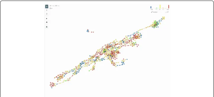
Analysis (TDA), a general framework to analyse
high-dimensional, incomplete and noisy data in a manner that
is less sensitive to the particular metric that is chosen,
and provides dimensionality reduction and robustness to
noise. TDA is embedded in the software produced by
the Ayasdi company to which the data were uploaded
[
113
]. As shown in Fig.
7
, the network of patients’
simi-larities obtained through TDA analysis and then colored
by the vital status of the patients at the end of the study
shows a higher level of complexity than is identified by
the clustering analysis, suggesting that statistical and/or
technical limitations of the clustering methods prevent
us to accurately represent reality.
Discussion
Multi-omics data integration is, among other
compo-nents of biological data integration, a very promising
and emerging field. We show a structured and effective
way to combine
‘omics data from multiple sources to
search for molecular profiles of patients. This process
allowed for the classification of a well-studied dataset of
OV. Other studies have been performed, either on this
same dataset [
114
–
118
], or on the same disease [
119
].
Tothill et al. in 2015 identified six clusters of patients,
based on mRNA, immunohistochemistry and clinical
data from a cohort of 285 Australian and Dutch
partici-pants, with a consensus clustering analysis of mRNA
data alone. The TCGA consortium produced their own
dataset in 2011, identifying four clusters based on
com-bined mRNA, miRNA and DNA methylation data (data
combined by summarising to the gene-level all datasets
through a factor analysis) and using a non-negative
matrix factorisation to identify clusters [
120
]. Further
analysis of the same dataset was then performed by
Zhang et al. [
118
], Jin et al. [
115
] and Kim et al. [
116
]
(with some variations), but these authors did not look
for new phenotypes in their analysis, rather comparing
data based on clinical endpoints (survival time,
histo-logical grades and stage of disease). Gevaert et al. [
114
]
used an original algorithm to combine DNA
methyla-tion, Copy Number Variation (CNV) and gene
expres-sion data, using the clusters defined in the TCGA
Table 4
Enrichment analysis for each comparison across all
‘
omics types, with q-values, and the literature references mentioning
involvement of the terms in ovarian cancer development. Q-values are the minimal false discovery rate at which the test may be
called significant, or in other words, the
p
-value threshold to satisfy the FDR criteria set by the Benjamini-Hochberg procedure
(Continued)
Term Term type ‘Omic type Contrast q-value Reference of implication in ovarian cancer hsa-miR-601 miRNA Transcriptomics 8 vs Rest 9.47E-07 [129]
hsa-miR-542-5p miRNA Transcriptomics 8 vs Rest 4.72E-04 [129] hsa-miR-361-3p miRNA Transcriptomics 8 vs Rest 1.07E-03 [129] hsa-miR-483-5p miRNA Transcriptomics 8 vs Rest 1.32E-03 [129] hsa-miR-769-5p miRNA Transcriptomics 8 vs Rest 1.68E-03 [129] Potassium signalling pathway Reactome Transcriptomics 8 vs Rest 1.15E-02 [163] hsa-miR-99b miRNA Transcriptomics 8 vs Rest 1.93E-02 [129] hsa-miR-339-3p miRNA Transcriptomics 8 vs Rest 2.28E-02 [129] T cell lineage commitment GO Biological Process Transcriptomics 8 vs Rest 3.80E-02 [164] hsa-miR-139-3p miRNA Transcriptomics 9 vs Rest 3.58E-09 [129] hsa-miR-423-5p miRNA Transcriptomics 9 vs Rest 5.89E-09 [129] hsa-miR-328 miRNA Transcriptomics 9 vs Rest 2.32E-08 [129] hsa-miR-370 miRNA Transcriptomics 9 vs Rest 4.83E-08 [129] hsa-miR-423-3p miRNA Transcriptomics 9 vs Rest 3.89E-06 [129] hsa-miR-940 miRNA Transcriptomics 9 vs Rest 5.37E-06 [129] hsa-miR-769-5p miRNA Transcriptomics 9 vs Rest 1.07E-04 [129] hsa-miR-339-3p miRNA Transcriptomics 9 vs Rest 0.000173 [129] hsa-miR-601 miRNA Transcriptomics 9 vs Rest 2.05E-04 [129] hsa-miR-483-5p miRNA Transcriptomics 9 vs Rest 7.33E-03 [129] Calcium signalling pathway KEGG pathways Transcriptomics 9 vs Rest 1.55E-02 [165] hsa-miR-542-5p miRNA Transcriptomics 9 vs Rest 1.69E-02 [129] cAMP signalling pathway KEGG pathways Transcriptomics 9 vs Rest 2.33E-02 [166] Ion transfer GO Biological Process Transcriptomics 9 vs Rest 3.43E-02 [167]
original paper. Those studies showed different ways of
analysing the data, leading to the identification of
clinic-ally relevant clusters in the case of Tothill and TCGA
original paper [
117
,
119
]. It is however the first time in
this paper that TCGA mRNA, miRNA and methylation
data were fused with an advanced data integration
method to identify robust subtypes of disease.
The number of clusters found in the same dataset
dif-fers between the TCGA analysis and our analysis. We
believe that the higher number of clusters we found is
the result of more up-to-date and powerful methods for
subtype discovery, as shown in the SNF original paper
[
55
]. Moreover, the subtypes identified in this analysis
do allow for a more in-depth classification of patients
linked with specific molecular subtypes than was
previ-ously reported. Building predictive models based on
multiple
‘omics profiles also contributes to the novelty
of this approach as other reported studies did not
pro-duce such a model, with the exception of the Tothill et
al. study [
119
] in which the authors developed a class
prediction model based on transcriptomics data only.
Clinically speaking, classifications are most useful when
they allow the identification of a subset of patients with a
clinically relevant outcome, such as low or high survival
rate, thus indicating where efforts may be focused to
de-velop new drugs, therapies and procedures. In our
ana-lysis, the groups identified after feature reduction are
statistically different in terms of survival rate and time.
For example, cluster 6 shows the highest rate of survival
among the 9 clusters identified and is associated with the
GPCR signalling pathway, cAMP, ion channels,
arachi-donic acid metabolism and a number of miRNAs (see
Table
4
or the Additional file
2
for more details).
Interestingly, while the two sets of groups defined with
or without feature reduction show differences in
inva-sion and clinical stage, statistically significant differences
in vital status are only detected amongst groups defined
with feature reduction. The reduced data also allows for
the definition of a higher number of stable groups (9
in-stead of 4), thereby pointing to the usefulness of
per-forming feature reduction prior to clustering analysis.
The biological functions highlighted by enrichment
analysis between the clusters indicate that these are
associated with different biological mechanisms leading
to the development of cancer in patients, ranging from
immune system disorders, cell cycle dysregulation,
im-paired response to DNA damage, modified energy
me-tabolism, etc.
The predictive models that were trained and tested
with two different methods gave mixed power results. In
the Random Forest case, the model could predict quite
well when patients did not belong to the clusters, but
not so well when patients did belong to them; in other
words, the model is specific but not sensitive. In the case
of the DIABLO PLS, the model is able to predict fairly
accurately the clusters 4 and 8 and less accurately cluster
5. Moreover, in the case of the DIABLO analysis, the
model showed that the clusters have different
‘omics
Fig. 7Network of patients shown in the TDA platform. The network is constructed as‘bins’grouping patients who are similar based on their‘omics profiles. Each dot in the network represents a bin. The bins are overlapping by an adaptable percentage, and if at least one patient is present in the overlap of two bins, the two bins will be linked in the network. The survival status of the patients is then translated as a color scheme (blue representing deceased patients and red alive patients). Using this technique, it is easy to identify‘islands’of good and poor survival among the patients, and equally easy to acknowledge that there are more such islands than is identified through the clustering technique. Thorough analysis of such networks can lead to insights into biology, as detailed in [168]