Heat Exchanger Network Cleaning Scheduling: From Optimal Control to
1
Mixed-Integer Decision Making
2
Riham Al Ismailia, Min Woo Leeb, D. Ian Wilsona, Vassilios S. Vassiliadisa,∗
3
aDepartment of Chemical Engineering and Biotechnology, University of Cambridge, Pembroke Street,
4
Cambridge CB2 3RA, United Kingdom
5
bDepartment of Chemical Engineering, Keimyung University, 1095 Dalgubeol-daero, Dalseo-gu, Daegu
6
42601, South Korea
7
Abstract
8
An approach for optimising the cleaning schedule in heat exchanger networks (HENs) subject
9
to fouling is presented. This work focuses on HEN applications in crude oil preheat trains
10
located in refineries. Previous approaches have focused on using mixed-integer nonlinear
11
programming (MINLP) methods involving binary decision variables describing when and
12
which unit to clean in a multi-period formulation. This work is based on the discovery that
13
the HEN cleaning scheduling problem is in actuality a multistage optimal control problem
14
(OCP), and further that cleaning actions are the controls which appear linearly in the system
15
equations. The key feature is that these problems exhibit bang-bang behaviour, obviating the
16
need for combinatorial optimisation methods. Several case studies are considered; ranging
17
from a single unit up to 25 units. Results show that the feasible path approach adopted is
18
stable and efficient in comparison to classical methods which sometimes suffer from failure
19
in convergence.
20
Keywords: Optimal control problem; Bang-bang control; Fouling; Optimisation;
21
Scheduling; Heat exchanger networks
22
1. Introduction
23
Fouling of heat transfer surfaces is a long-established problem and has been described
24
as “the major unresolved problem in heat transfer” (Taborek et al., 1972). It is one of the
25
most significant issues affecting heat exchanger operation and thus has been depicted as “a
26
nearly universal problem in heat exchanger equipment and design” (Watkinson, 1988). Heat
27
exchanger fouling accounts for 0.25% of gross national product (GNP) in highly industrialised
28
countries (Pugh et al., 2001).
29
This major industry-wide problem is caused by the deterioration in heat transfer resulting
30
from fouling and leads to the loss of efficiency in heat exchangers which must be offset. This
is achieved through process turndown, increased utility consumption with affiliated surge
32
in greenhouse gas emissions until operation requirements such as temperature and
pump-33
around targets are met, or in extreme cases plant shutdown. The reduction of production
34
rates and increased energy consumption lead to economic losses which are more significant
35
in larger networks of heat exchangers that require long continuous operational times between
36
shutdowns, particularly crude distillation unit preheat trains (PHT) on oil refineries (Smaïli
37
et al., 2001).
38
Based on 1995 figures, the costs associated specifically with crude oil fouling in PHT
39
worldwide were estimated to be of the order of 4.5 billion USD (Pugh et al., 2001).
Foul-40
ing mitigation techniques include addition of antifoulant chemicals, using more robust heat
41
transfer equipment, and regular cleaning of fouled units. Cleaning of heat exchangers has
42
a negative impact on operating costs due to the unit being taken offline, however with the
43
development of optimisation strategies such as those proposed by Casado (1990), Smaïli et al.
44
(1999),Georgiadis and Papageorgiou (2000), Lavaja and Bagajewicz (2004), Ishiyama et al.
45
(2009b), Gonçalves et al. (2014), among others, these costs can be minimised resulting in
46
overall gains due to improved heat transfer of the network over time.
47
The cleaning scheduling problem is a discrete decision making problem where a decision
48
must be made as to whether cleaning should be performed, and which unit is to be cleaned.
49
It consists of continuous as well as binary decision variables and hence it has combinatorial
50
complexity that is handled traditionally by Branch and Bound (B&B) methods of one form
51
or another. Due to its combinatorial nature and the existence of nonlinear models,
mathem-52
atical programming (MP) techniques have been used to solve this mixed integer nonlinear
53
programming (MINLP) problem based on time discretisation (Smaïli et al., 2001).
Addi-54
tionally this problem has been solved by formulating certain models from a MINLP model
55
to a mixed integer linear programming (MILP) model (Georgiadis and Papageorgiou, 2000).
56
Stochastic optimisation frameworks using distinctive modifications of simulated annealing
al-57
gorithms have been implemented (Smaïli et al., 2002a) as well as heuristic schemes composed
of a set of movements according to a greedy rationale (Gonçalves et al., 2014).
59
This problem has been addressed in the literature through extending the formulation
60
of the general cleaning scheduling problem in a multitude of ways. Rodriguez and Smith
61
(2007) combined the conventional cleaning scheduling problem with optimisation of operating
62
conditions such as wall temperature and flow velocity in a comprehensive mitigation strategy
63
while Ishiyama et al. (2010) considered the addition of the problem of controlling the desalter
64
inlet temperature by using hot stream bypassing within a PHT fouling mitigation strategy
65
based on heat exchanger cleaning.
66
Certain formulations include constraints set by pump-around operation (Smaïli et al.,
67
2002a) and pressure drop (Smaïli et al., 2001), while both thermal and hydraulic impacts of
68
fouling were considered by Ishiyama et al. (2009b) where variable throughput and control
69
valve operation are implemented on the cleaning scheduling problem.
70
A cleaning operation will ideally remove all fouling deposits from a heat transfer surface.
71
In practice the effectiveness of a cleaning operation depends on the nature of the deposit and
72
the method of cleaning. Ishiyama et al. (2011) presented a framework for incorporating this
73
complexity into the scheduling problem. The replacement of the single layer fouling model
74
with a dual layer consisting of a soft exterior deposit (gel) and a harder interior layer (coke)
75
was investigated by Pogiatzis et al. (2012). They considered the case where two cleaning
76
methods were available: (a) cleaning-in-place methods and (b) off-line mechanical cleaning.
77
An extra decision variable is added to the scheduling model, capturing the choice of cleaning
78
method. The current paper addresses a single layer fouling model where the fouling kinetics
79
exhibit linear and asymptotic behaviour.
80
Current solution methods for the cleaning scheduling problem still present limitations.
81
Due to the complexity of networks and the nonlinearity in the models, MINLP approaches
82
sometimes suffer from failure in convergence (Georgiadis and Papageorgiou, 2000; Smaïli
83
et al., 2001) whereas MILP techniques may be computationally expensive (Lavaja and
Baga-84
jewicz, 2004) and involve the introduction of approximations to models. For example,
giadis and Papageorgiou (2000) used the arithmetic temperature difference instead of the
86
logarithmic mean temperature difference, which is not suitable for large networks that
fea-87
ture extensive feedback of hot (and/or cold) streams (Smaïli et al., 2001).
88
Stochastic optimisation methods may not be capable of handling problems involving many
89
variables of similar effect (Fouskakis and Draper, 2002). Furthermore, these approaches can
90
be very dependent on parameter tuning (Gonçalves et al., 2014). Solutions found by heuristic
91
schemes such as greedy algorithms are not guaranteed to be optimal. For the scheduling
92
problem, such simple strategies consider cleaning actions only in the current period and may
93
be inefficient (Smaïli et al., 2001). Therefore, there is a need to develop robust, reliable and
94
inexpensive methods to solve the scheduling cleaning problem.
95
In this paper we show for the first time that the heat exchanger network (HEN)
clean-96
ing scheduling problems are in actuality mixed-integer optimal control problems (MIOCPs)
97
which exhibit a nearly bang-bang solution. This paper is arranged as follows: section 2
de-98
scribes the formulation as a multi-period optimal control problem (OCP), including the proof
99
of linearity of the control resulting in this bang-bang optimal solution behaviour. The
formu-100
lation considered for the general HEN cleaning scheduling problem is presented in section 3.
101
Implementation and solutions to a number of case studies for crude oil PHT obtained using
102
a commercial optimisation software are presented in sections 4 and 5, including comparison
103
of solutions to those produced through MP techniques.
104
2. HEN Scheduling Optimisation as Multi-period Optimal Control
105
This section will demonstrate that the HEN cleaning scheduling problem is in actuality
106
a MIOCP. In this problem the controls, i.e. cleaning decisions occur linearly in the system,
107
thus resulting in a bang-bang solution. Hence, integrality of the solution can be obtained by
108
solving only the relaxed MIOCP as a standard nonlinear programming (NLP). Furthermore,
109
proof of linearity in the control is shown in this section.
110
The basic formulation for an OCP is expressed in equations (1a) to (1d) where the
formance index is minimised by selection of controls u(t)subject to differential and algebraic
112
equations involving differential and algebraic state variablesx(t)andy(t), respectively.
Equa-113
tions (1b) to (1c) describe an index-1 differential algebraic equation (DAE) system given the
114
initial conditionx0, and a fixed final timetF. It is noted that the problem considered involves
115
binary control variables, u(t), thus constituting a MIOCP.
116 min u(·)O =φ[x(tF)]+ tF ˆ 0 L[x(t), y(t), u(t), t]dt (1a) subject to 117 ˙ x(t) = f[x(t), y(t), u(t), t], x(t0) =x0, (1b) g(x(t), y(t), u(t), t) = 0, (1c) u(t)∈ U, U ∈ {0,1} ∀t ∈[0, tF] (1d)
The OCP solution is obtained through discretisation of time into periods, where the
118
control profiles are allowed to be discontinuous at a finite number of points, tp, termed
119
junctions. Period lengths have not been specified. Vassiliadis (1993) gives a general form of
120
junction conditions between stages (i.e. periods) p and p+ 1. This is shown in equation 2
121
for the sake of clarity.
122
Jp( ˙xp+1(tp+), xp+1(t+p), yp+1(t+p), up+1(t+p),x˙p(t−p), xp(t−p), yp(t−p), up(t−p), tp) = 0 ∀p= 1,2, . . . , N P−1
(2)
The basic formulation of a multi-period OCP over time periods, p = 1, . . . , N P, t ∈
123
[tp−1, tp] with tN P =tF is shown in equations (3a) to (3g).
min u(·) O = N P X p=1 φ(p)x(tp), y(p)(tp), u(p), t(p) + tp ˆ tp−1 L(p)x(p)(t), y(p)(t), u(p), t dt (3a) subject to 125 ˙ x(p)(t) = f(p)(x(p)(t), y(p)(t), u(p), t) (3b) 0 =g(p)(x(p)(t), y(p)(t), u(p), t) (3c) tp−1 ≤t≤tp, p= 1,2, . . . , N P (3d) x(1)(t0) =I(1)(u(1)) (3e) x(p)(tp−1) = I(p)(x(p−1)(tp−1), y(p−1)(tp−1), u(p)) ∀p= 2,3, . . . , N P (3f) u(t)∈ U, U ∈ {0,1} (3g)
For the HEN cleaning problem the controlsu(p)t are considered to be piecewise constant
126
so as to reflect the on/off nature of having a unit cleaning or not. The stage switching times
127
tp are fixed in this initial derivation. The collective vector of controls over all stages is:
128
u= ((u(1))T,(u(2))T, . . . ,(u(N P))T)T (4)
At the junctions, conditions are set where differential state variables are allowed to be
129
reinitialised based on the control variable value:
xp(tp−1) = up(t)·xp−1(tp−1) ∀p= 2, . . . N P (5)
Proof that the control in the relaxed multistage MIOCP for cleaning scheduling is linearly
131
related to the process variables is provided as follows:
132
This multistage adjoint system is a linear time-varying coefficient semi-explicit index-1
133
DAE system. The performance index in equation (3a) is modified such that the
Euler-134
Lagrange multipliers are introduced:
135 ¯ O = N P X p=2 ( φ(p)(x(p)(tp), y(p)(tp), u(p), t(p)) + λ(p)(tp−1) T · I(p)(x(p−1)(tp−1), y(p−1)(tp−1), u(p))−x(p)(tp−1) + ˆ tp tp−1 L(p)(x(p)(t), y(p)(tp), u(p), t)dt + ˆ tp tp−1 λ(p)(t)T · f(p)(x(p)(t), y(p)(tp), u(p), t)−x˙(p)(t) dt + ˆ tp tp−1 µ(p)(t)T · g(p)(x(p)(t), y(p)(t), u(p), t) dt ) +φ(1)(x(1)(t1), y(1)(t1), u(1), t(1)) + λ(1)(t0) T · I(1)(u(1))−x(1)(t0) + ˆ t1 t0 L(1)(x(1)(t), y(1)(t), u(1), t)dt + ˆ t1 t0 λ(1)(t)T · f(1)(x(1)(t), y(1)(t), u(1), t)−x˙(1)(t) dt + ˆ t1 t0 µ(1)(t)T · g(1)(x(1)(t), y(1)(t), u(1), t) dt (6)
Variations on the parameter set of stagep0, of the formδu(p0) are considered, which result
136
in variations in the state values at all times as shown in equation (7). Clearly, the state vector
of stagep , wherep < p0, will not be influenced. This results inδx(p)(t),0andδy(p)(t),0. 138 δO¯ = N P X p=2 ( ∂φ(p) ∂x(p)(t p) δx(p)(tp) + ∂φ(p) ∂y(p)(t p) δy(p)(tp) + ∂φ(p) ∂u(k)δu (p) + λ(p)(tp−1) T · ∂I(p) ∂x(p−1)(t p−1) δx(p−1)(tp−1) + ∂I(p) ∂y(p−1)(t p−1) δy(p−1)(tp−1) + ∂I(p) ∂u(p)δu (p)−δx(p)(t p−1) + ˆ tp tp−1 ∂L(p) ∂x(p)(t)δx (p)(t) + ∂L (p) ∂y(p)(t)δy (p)(t) + ∂L (p) ∂u(p)δu (p)dt + ˆ tp tp−1 λ(p)(t)T · ∂f(p) ∂x(p)(t)δx (p)(t) + ∂f(p) ∂y(p)(t)δy (p)(t) + ∂f(p) ∂u(p)δu (p)−δx˙(p)(t) dt + ˆ tp tp−1 µ(p)(t)T · ∂g(p) ∂x(p)(t)δx (p)(t) + ∂g(p) ∂y(p)(t)δy (p)(t) + ∂g(p) ∂u(p)δu (p) dt ) + ∂φ(1) ∂x(1)(t 1) δx(1)(t1) + ∂φ(1) ∂y(1)(t 1) δy(1)(t1) + ∂φ(1) ∂u(1)δu (1) + λ(1)(t0) T · ∂I(1) ∂u(1)δu (1)−δx(1)(t 0) + ˆ t1 t0 ∂L(1) ∂x(1)(t)δx (1)(t) + ∂L(1) ∂y(1)(t)δy (1)(t) + ∂L(1) ∂u(1)δu (1)dt + ˆ t1 t0 λ(1)(t)T · ∂f(1) ∂x(1)(t)δx (1)(t) + ∂f (1) ∂y(1)(t)δy (1)(t) + ∂f (1) ∂u(1)δu (1)−δx˙(1)(t) dt + ˆ t1 t0 µ(1)(t)T · ∂g(1) ∂x(1)(t)δx (1)(t) + ∂g(1) ∂y(1)(t)δy (1)(t) + ∂g(1) ∂u(1)δu (1) dt (7)
Integration by parts for the last term in the integrals involving δx˙(p) is used to obtain
139
equation (8):
δO¯ = N P X p=2 ( ∂φ(p) ∂x(p)(t p) δx(p)(tp) + ∂φ(p) ∂y(p)(t p) δy(p)(tk) + ∂φ(p) ∂u(p)δu (p) + λ(p)(tp−1) T · ∂I(p) ∂x(p−1)(t p−1) δx(p−1)(tp−1) + ∂I(p) ∂y(p−1)(t p−1) δy(p−1)(tp−1) + ∂I(p) ∂u(p)δu (p)−δx(p)(t p−1) + ˆ tp tp−1 ∂L(p) ∂x(p)(t)δx (p)(t) + ∂L(p) ∂y(p)(t)δy (p)(t) + ∂L(p) ∂u(p)δu (p)dt + ˆ tp tp−1 λ(p)(t)T · ∂f(p) ∂x(p)(t)δx (p)(t) + ∂f(p) ∂y(p)(t)δy (p)(t) + ∂f(p) ∂u(p)δu (p) dt + ˆ tp tp−1 ˙ λ(p)(t) T δx(p)(t)dt + λ(p)(tp−1) T ·δx(p)(tp−1)− λ(p)(tp) T ·δx(p)(tp) + ˆ tp tp−1 µ(p)(t)T · ∂g(p) ∂x(p)(t)δx (p)(t) + ∂g(p) ∂y(p)(t)δy (p)(t) + ∂g(p) ∂u(p)δu (p) dt ) + ∂φ(1) ∂x(1)(t 1) δx(1)(t1) + ∂φ(1) ∂y(1)(t 1) δy(1)(t1) + ∂φ(1) ∂u(1)δu (1) + λ(1)(t0) T · ∂I(1) ∂u(1)δu (1)−δx(1)(t 0) + ˆ t1 t0 ∂L(1) ∂x(1)(t)δx (1) (t) + ∂L (1) ∂y(1)(t)δy (1) (t) + ∂L (1) ∂u(1)δu (1) dt + ˆ t1 t0 λ(1)(t)T · ∂f(1) ∂x(1)(t)δx (1)(t) + ∂f(1) ∂y(1)(t)δy (1)(t) + ∂f(1) ∂u(1)δu (1) dt + ˆ t1 t0 ˙ λ(1)(t) T δx(1)(t)dt + λ(1)(t0)T ·δx(1)(t0)− λ(1)(t1)T ·δx(1)(t1) + ˆ t1 t0 µ(1)(t)T · ∂g(1) ∂x(1)(t)δx (1)(t) + ∂g (1) ∂y(1)(t)δy (1)(t) + ∂g (1) ∂u(1)δu (1) dt (8)
For a stationary point, infinitesimal variations in the right hand side should yield no
141
change to the performance index, i.e. δO¯ = 0, and hence related terms must be chosen so
that they always guarantee this. This leads to the following set of Euler-Lagrange equations
143
and the Pontryagin et al. (1962) maximum (minimum) principle.
144
To cancel the δx(1)(t) and δx(1)(t1) terms, the differential equations and final time stage
145
conditions as shown in equations (9a) to (10) must hold, respectively:
146 ˙ λ(1)(t) =− ∂f(1) ∂x(1)(t) T λ(1)(t)− ∂g(1) ∂x(1)(t) T µ(1)(t)− ∂L(1) ∂x(1)(t) T (9a) t0 ≤t≤t1 (9b) λ(1)(t1) = ∂φ(1) ∂x(1)(t 1) T (10) Algebraic equations and final stage conditions (11a) to (11b) must hold in order to cancel
147
the δy(1)(t) and δy(1)(t
1) terms; 148 ∂f(1) ∂y(1)(t) T λ(1)(t) + ∂g(1) ∂y(1)(t) T µ(1)(t) + ∂L(1) ∂y(1)(t) T = 0 (11a) t0 ≤t≤t1 (11b) ∂φ(1) ∂y(1)(t 1) T + ∂I(2) ∂y(1)(t 1) T ·λ(2)(t1) = 0 (12)
The δx(p)(t) and δx(p)(tp) terms are cancelled through the condition that the following
dif-149
ferential equations and final time stage conditions are held;
150 ˙ λ(p)(t) =− ∂f(p) ∂x(p)(t) T λ(p)(t)− ∂L(p) ∂x(p)(t) T (13a) 151 tp−1 ≤t ≤tp ∀p= 2,3, . . . N P (13b)
λ(p)(tp) = ∂φ(p) ∂x(p)(t p) T + ∂I(p+1) ∂x(p)(t p) T ·λ(p+1)(tp) ∀p= 2,3, . . . , N P −1
To cancel δy(p)(t)and δy(p)(tp) terms, the following algebraic equations must hold:
152 ∂f(p) ∂y(p)(t) T λ(p)(t) + ∂g(p) ∂y(p)(t) T µ(p)(t) + ∂L(p) ∂y(p)(t) T = 0 tp−1 ≤t ≤tp ∀p= 2,3, . . . N P ∂φ(p) ∂y(p)(t p) T + ∂I(p+1) ∂y(p)(t p) T ·λ(p+1)(tp) = 0 ∀p= 2,3, . . . , N P −1
The terms δu(1) and δu(p) are cancelled on the condition that equations (15a) to (16b) hold.
153
These are equivalent to the Hamiltonian gradient condition:
154 ∂φ(1) ∂u(1)(t1) T + ∂I(1) ∂u(1) T ·λ(1)(t0) + ˆ t1 t0 ( ∂L(1) ∂u(1)(t) T + ∂f(1) ∂u(1)(t) T ·λ(1)(t) + ∂g(1) ∂u(1)(t) T ·µ(1)(t) ) dt= 0 (15a) t0 ≤t≤t1 (15b) ∂φ(p) ∂u(p)(tp) T + ∂I(p) ∂u(p) T ·λ(p)(tp−1) + ˆ tp tp−1 ( ∂L(p) ∂u(p)(t) T + ∂f(p) ∂u(p)(t) T ·λ(p)(t) + ∂g(p) ∂u(p)(t) T ·µ(p)(t) ) dt = 0 (16a)
tp−1 ≤t ≤tp ∀p= 2,3, . . . N P (16b)
When the functions appearing in equations (15a) and (16a) are linearly related to the
155
control, the optimal control for the relaxed MIOCP will exhibit bang-bang behaviour (with
156
potential singular arcs). Bang-bang solutions occur when the optimal control action is at
157
either bound of the feasible region (Bryson and Ho, 1975). Controls that are not
bang-158
bang, where the control lies between the bounds, are called singular. In this case, singular
159
arcs exist. Pure bang-bang controls are demonstrated in minimum-time problems for linear
160
systems (Bellman et al., 1956) and bilinear systems (Mohler, 1973), optimal control of batch
161
reactors (Blakemore and Aris, 1962), optimal thermal control (Belghith et al., 1986), etc.
162
For nonlinear optimisation systems, this bang-bang principle does not always hold. Zandvliet
163
et al. (2007) investigated reservoir flooding problems, where the control is linear in relation
164
to the continuous variables, and showed that if the only constraints are upper and lower
165
bounds on the control, then due to their particular structure, these problems will sometimes
166
have bang-bang optimal solutions. This is advantageous since bang-bang solutions can be
167
implemented with simple on–off control valves.
168
Approaches for optimal control of nonlinear dynamical systems with binary controls (on/off)
169
were reviewed by Sager (2009). To satisfy requirements for bang-bang behaviour, the general
170
OCP is reformulated such that the binary controls are presented linearly in the system
171
dynamics. Solutions in this case may require use of heuristics e.g. rounding up or a sum
172
up rounding strategy, or algorithms such as Branch and Bound when singular arcs appear
173
(Sager, 2009).
174
For the scheduling cleaning problem, reformulation is not necessary as the controls involved
175
already have linear presentation in the system. More importantly, the formulation of this
176
problem as an OCP facilitates the solution of the relaxed nonlinear programming (NLP)
177
problem through the feasible path approach, obviating the need to discretise the system
178
equations. This otherwise leads to a very large scale optimisation problem with a strongly
nonlinear system of equality constraints. This approach avoids failures of convergence
pro-180
duced by direct solutions of MINLPs resulting from discretisation, such as in previous work
181
of Georgiadis and Papageorgiou (2000) and of Smaïli et al. (2001).
182
3. HEN Scheduling Optimisation Formulation
183
The effect of fouling on heat transfer performance is often quantified in lumped parameter
184
models of process heat transfer via the fouling resistance, Rf.
185 186 1 U = 1 Uc +Rf (17)
Equation (17) expresses the overall heat transfer coefficient U in relation to the fouling
187
resistance and Uc, its value when clean.
188
The impact of fouling resistance is more severe for heat exchangers with a high overall
189
heat transfer coefficient. Both linear (equation (18)) and exponentially asymptotic fouling
190
behaviour (equation (19)) are considered in this paper , which are quantified via
191
˙
Rf =a (18)
Rf=R∞f (1−exp(−t0/τ)) (19)
where a is the linear fouling constant for a particular heat exchanger, R∞f is the asymptotic
192
fouling resistance, τ is the decay constant, andt0 is the operating time elapsed since the last
193
cleaning action.
194
The heat duty of a single-pass shell and tube heat exchanger operating in counter-current
195
mode is given by equation (20), which is based on the log-mean temperature difference
196
method.
197 198
Q=U A4Tlm (20)
Here A is the area and 4Tlm is the logarithmic mean temperature difference.
The heat duty,Q, is also linearly related to the stream inlet and outlet temperatures through
200
the energy balances outlined in equations (21) and (22):
201 202
Q=FcCc(Tcout−Tcin) (21)
203
Q=FhCh(Thin−Thout) (22)
where Fh and Fc are the mass flow-rates of the hot and cold streams respectively, and Ch
204
and Cc are their specific heat capacities.
205
The cleaning scheduling problem is a multi-period OCP where a decision must be made
206
regarding when, i.e. in which period(s), cleaning should occur, and which unit is to be
207
cleaned. The control action is discretised into time periods of equal length, where each
208
period is discretised further into a cleaning and operating sub-period. This is represented by
209
binary variable ynp which is used to describe the cleaning status of each exchanger in each
210
cleaning sub-period, where
211 ynp =
0 if the nth heat exchanger is cleaned in periodp
1 otherwise ∀n, p (23)
Within an operating sub-period, this binary variable is fixed to 1 for all n i.e. all units are
212
online. The objective is to minimise the operating and cleaning costs due to fouling over
213
a specified horizon of time tF. The objective function is given by equation (24). The form
214
of this objective function is generally common to all approaches. Local considerations may
215
give slightly different mathematical expressions. However, the differences lie in the solution
216 approach. 217 218 Obj = tF ˆ 0 CEQF(t) ηf dt+ N P X p=1 N E X n=1 Cc(1−ynp) (24)
The extra furnace energy consumption is described by the term QF(t) which is determined
219
based on the temperature of the crude oil entering the furnace, i.e. the crude inlet
temper-220
ature (CIT). CE represents the cost of fuel, ηf is the furnace efficiency, N E is the number
of exchangers considered for cleaning, N P is the number of periods, and Cc is the cost per
222
cleaning action. For the purpose of attaining results that can be compared to published ones
223
from case studies in the open literature, Cc is taken to be independent of the exchanger size
224
and duty. In industrial practice this is not the case, as larger exchangers take more effort to
225
clean and will thus have a higher value of Cc and vice versa. The amount of time taken to
226
clean depends on the installation: if the exchanger must be isolated, removed and relocated
227
for cleaning, these operations can determine the cleaning time. Furthermore, different
clean-228
ing methods will have different durations, but this is not considered in this work. Through
229
incorporation of binary variable ynp, equations (18) and (19) can be rewritten as:
230 ˙ Rf =ynpa ∀n, p (25) Rf=R∞f (1−exp(−t0/τ)) (26a) ˙ t0 =y np ∀n, p (26b)
The HEN optimisation is started from a clean condition,i.e. the initial fouling resistance
231
is 0 for the first period for all heat exchangers. In consecutive periods, the initial fouling
232
resistance is related to the fouling resistance at the end of the previous period by integration
233
in time and this value is allowed to be reset through a junction condition when cleaning
234
occurs.
235
The number of transfer units (NTU) effectiveness method is used to assess the performance
236
of each heat exchanger. This is achieved by rearranging equation (20) in terms of a rating
237
calculation. The units are modelled as simple countercurrent exchangers. The effectiveness
238
term denoted by α and the ratio of capacity flow-ratesP defined by equations (27) and (28)
239
are reproduced from Smaïli et al. (2001) :
240 241
α= U A
P = FhCh
FcCc (28)
Through combination and rearrangement of equations (20), (21) and (22) the temperature
242
of the hot and cold streams leaving each exchanger can be calculated. The temperatures of
243
the cold and hot streams leaving an exchanger are determined by:
244 245 Tcout =Tcin+P Thin−Thout (29) 246 Thout = ynp (1−P)Thinexp(−α(1−P)) +Tcin(1−exp(−α(1−P))) 1−P exp(−α(1−P)) (30) +(1−ynp)Thin ∀n, p
The above equations are applicable to most preheat configurations which feature P < 1. If
247
the alternative case arises, these equations must be amended.
248
4. Implementation
249
The implementation is performed in MATLAB®R2016b with its Optimisation ToolboxTM
250
and Parallel Computing ToolboxTM(The MathWorks Inc., 2016). It is noteworthy that this
251
methodology cannot be implemented in current commercial simulators directly. For example,
252
gPROMSTM(Process Systems Enterprise, 2017), which is one of the most advanced
commer-253
cial simulators, does not facilitate multi-period optimal control problem solutions as it does
254
not allow for junction conditions.
255
The MATLAB® code works as a standard multi-period optimal control problem solver
256
using the feasible path approach (i.e. sequential approach) by linking together the Ordinary
257
Differential Equation (ODE) solver ode15s with the optimiser fmincon. The default
set-258
tings for ode15s are used, with absolute tolerance of 10-6 and relative tolerance of 10-3. The
259
optimiser fmincon is used with the Sequential Quadratic Programming (SQP) algorithm
op-260
tion whilst keeping the remaining settings at their default values: constraint, optimality and
261
step tolerances of 10-6 using a forward finite difference scheme for the estimation of
ents. Gradient evaluations conducted via finite differences are costly and require repeated
263
simulations of the dynamic process model.
264
Additionally, since this problem is non-convex, multiple runs with different starting points
265
are performed and the best solution is reported. A test was run using the Parallel Computing
266
ToolboxTMto compare the computational time between parallelisation of the gradient
evalu-267
ations versus parallelising a loop of multiple starting points. On a 4GHz Intel Core i7, 16 GB
268
RAM iMac running on macOS Sierra the latter was faster than the former. Parallelisation
269
of a loop of 50 runs is performed using a parfor loop. For cases where singularities appear in
270
the control, a rounding up scheme is employed.
271
5. Case Studies
272
Computation experiments for the scheduling of cleaning actions for HENs located in
273
crude oil distillation unit PHTs undergoing fouling are considered here. We present case
274
studies appearing in the work of Lavaja and Bagajewicz (2004): a single heat exchanger
275
unit; 4 units in series, a network of 10 units; and the more complex network of 25 units
276
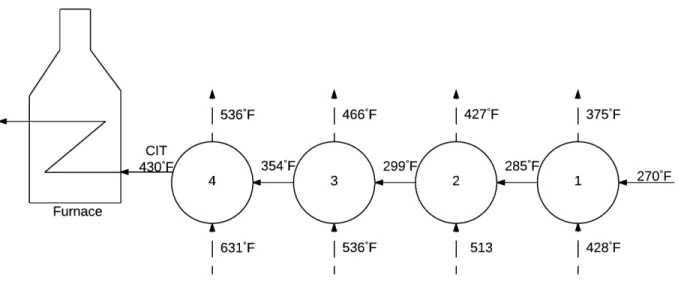
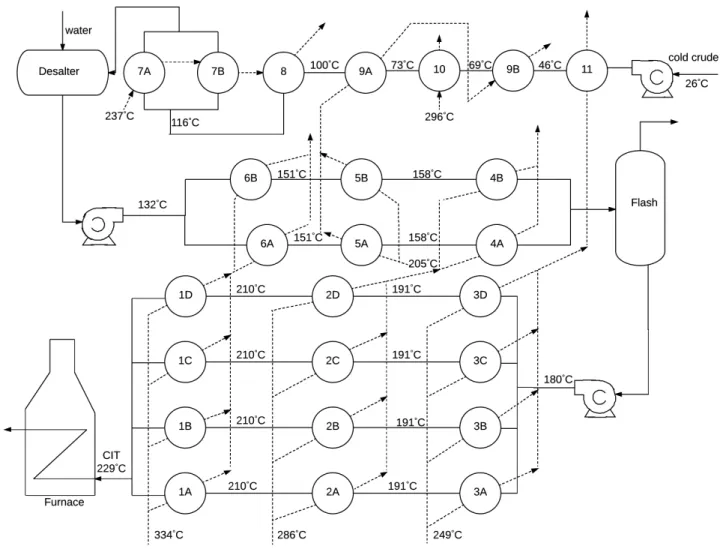
presented by Smaïli et al. (2002a). These are shown in figures 1 to 3. Stream data for each
277
model are presented in tables 1 to 3 and 5. For the 10 unit HEN case study presented in
278
the Lavaja and Bagajewicz (2004) formulation and the 25 unit HEN case study presented
279
in the Smaïli et al. (2002a) formulation, the selection and operational constraints imposed
280
through consideration of performance targets or acceptable operating practice are shown in
281
tables 4 and 6, respectively. These constraints are based only on exchanger cleaning actions.
282
However, in practice temperature bounds on the performance of exchangers are required to
283
be applied, for example in the case of desalter temperature control considered by Ishiyama
284
et al. (2010). For the purpose of achieving results that can be compared to published ones
285
from case studies in the open literature, only the constraints shown in tables 4 and 6 are
286
imposed on the corresponding case studies.
287
The number of periods considered is N P = 24 for the single unit and N P = 18 for the
10 unit HEN case studies while this is N P = {12,18} for the 4 unit heat exchanger case 289
study. A longer duration is considered for the 25 unit HEN, withN P = 36. Both linear and
290
asymptotic fouling models are considered in the single unit and 10 unit HEN cases whilst
291
only linear fouling is modelled in the 4 units and 25 unit HEN case studies. This is done for
292
comparison purposes.
293
The extra energy cost required due to fouling CE in the objective function displayed in
294
equation (24) is £0.34/kW day for the 25 unit HEN case. There is no mention of the furnace
295
fuel cost in the work of Lavaja and Bagajewicz, so a cost of £2.93/MM Btu is used here based
296
on the value reported by Smaïli et al. (2002b). The work of Smaïli et al. is the source of
297
data for Lavaja and Bagajewicz’s models where they compared the solutions from their MILP
298
approach with those obtained by Smaïli et al. using the OA/ER algorithm. Although Lavaja
299
and Bagajewicz stated that they accounted for the decay in the heat transfer coefficient in
300
each sub-period, expressed by ηc, there is no mention of the value of this parameter in their
301
work. Hence, we considered the value of parameter ηc to be 1 in our model. This decay
302
parameter is also fixed at the value of 1 in the 25 unit HEN case study along with the
303
furnace efficiency ηf. Smaïli et al. (2002b) did not consider these parameters in their model.
304
The cleaning cost incurred for cleaning operations,Cc, is £5000 per cleaning action in the 25
305
unit HEN case and £4000 for all other cases. For the former case, the duration of the cleaning
306
and operating sub-periods are equal with 4tcl = 4top = 15 days. If the cleaning time did
307
depend on the size of the exchanger, these durations would have to be unit dependent.
308
The scheduling problem was reformulated into a MILP problem by Lavaja and Bagajewicz
309
(2004) whereas Smaïli et al. (2002a) solved the MINLP problem directly using two methods:
310
a Backtracking Threshold Accepting (BTA) algorithm and the Outer Approximation (OA)
311
method.
Figure 1: Four heat exchanger case. Temperature values are given for initial, clean condition. Adapted from Lavaja and Bagajewicz, 2004.
Figure 2: 10 unit HEN case. Temperature values are given for initial, clean condition. Adapted from Lavaja and Bagajewicz, 2004.
Figure 3: 25 unit HEN case. Solid lines, cold (crude) streams; dashed lines, hot streams; CIT, crude inlet temperature to furnace. Temperature values are given for initial, clean condition. Adapted from Smaïli et al., 2002a.
The cleaning schedules featuring the best objective, i.e. lowest overall cost, are reported
313
for each case. The optimal cleaning schedules are presented in tables 11 to 16 alongside
314
those obtained by Lavaja and Bagajewicz (2004) and Smaïli et al. (2002a). In the economic
315
comparison, we placed the cleaning schedules obtained by Lavaja and Bagajewicz (2004) and
316
Smaïli et al. (2002a) into our model to evaluate the cost. Tables 7 to 10 show the economic
317
comparison.
318
Fouling rates directly impact the performance of heat exchangers. The asymptotic fouling
319
cases have larger initial fouling rates, causing a rapid decay in the hot stream temperatures
320
through the network, resulting in a much larger objective value for the uncleaned case (e.g.
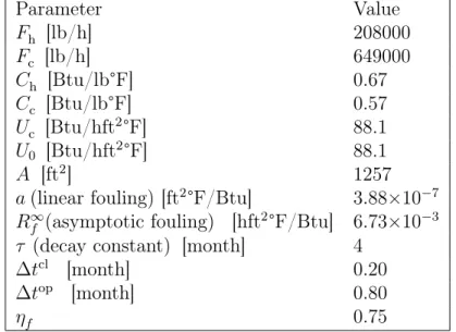
Table 1: Data for single heat exchanger case. Adapted from Lavaja and Bagajewicz, 2004. Parameter Value Fh [lb/h] 208000 Fc [lb/h] 649000 Ch [Btu/lb°F] 0.67 Cc [Btu/lb°F] 0.57 Uc [Btu/hft2°F] 88.1 U0 [Btu/hft2°F] 88.1 A [ft2] 1257
a(linear fouling) [ft2°F/Btu] 3.88×10⁻⁷
Rf∞(asymptotic fouling) [hft2°F/Btu] 6.73×10⁻³
τ (decay constant) [month] 4
∆tcl [month] 0.20
∆top [month] 0.80
ηf 0.75
£317k vs. £203k for the single unit case shown in table 7). Consequently, one would expect
322
more cleaning actions in all the asymptotic fouling model cases than the corresponding linear
323
ones due to the early loss of exchanger efficiencies. This is evident in table 11 with the cleaning
324
actions increasing from 3 to 5 in both this work’s solution and the solution of Lavaja and
325
Bagajewicz (2004). Similar observations to Lavaja and Bagajewicz (2004) are seen in the
326
single unit case, where cleaning actions are cyclic (table 11). For linear fouling, the number
327
of cleaning actions as well as the schedules are very similar: however the cleanings in our
328
model are performed 1 month earlier than in Lavaja and Bagajewicz ’s schedule.
329
For the four heat exchanger case, the number of cleaning actions are the same as Lavaja
330
and Bagajewicz ’s model and the schedule for the 12 month operating horizon is the same,
331
meanwhile the schedule for the 18 month duration differs. No pattern is evident when the
332
schedules are compared, with some cleaning actions occurring earlier in some cases and later
333
in others.
334
In the majority of our cases our model produced similar overall costs to those reported
335
by Lavaja and Bagajewicz (2004), the only differences being (i) the 4 heat exchanger case
336
over 18 months, where the cost of our schedule is slightly smaller than that reported, with
337
the difference in savings being only <1.5%; and (ii) the 10 unit HEN case with asymptotic
T able 2: Data for four heat exc hangers case. Repro duced from La v a ja and Baga jewicz, 2004. Parameter Heat Exc hanger 1 2 3 4 Fh [lb/h] 141000 73800 423000 429000 Ch [Btu/lb °F] 0.67 0.70 0.62 0.62 A [ft 2 ] 465 287 1192 1488 a ( linear fouling, × 10 7 ) [ft 2 °F/Btu] 3.07 3.27 3 . 68 3.88 Fc [lb/h] 721000 Cc [Btu/lb °F] 0.46 Uc [Btu/hft 2 °F] 88.1 U0 [Btu/hft 2 °F] 88.1 ∆ t cl [mon th] 0.20 ∆ t op [mon th] 0. 80
T able 3: Data for 10 unit HEN case. A dapted from La v a ja and Ba ga jewicz, 2004. Parameter Heat Exc hanger 1 2 3 4 5 6 7 8 9 10 Fh [lb/h] 141000 73800 423000 429000 208000 423000 210000 141000 283000 208000 Fc [lb/h] 721000 721000 721000 721000 721000 721000 721000 649000 649000 649000 Ch [Btu/lb °F] 0 . 67 0 . 70 0 . 62 0 . 62 0 . 67 0 . 62 0 . 69 0 . 67 0 . 69 0 . 67 Cc [Btu/lb °F] 0 . 46 0 . 46 0 . 46 0 . 46 0 . 55 0 . 55 0 . 55 0 . 57 0 . 57 0 . 57 A [ft 2 ] 465 287 1192 1488 183 546 492 437 885 1257 a ( linear fouling, × 10 7 ) [ft 2 °F/Btu] 1 . 23 1 . 84 1 . 23 1 . 64 3 . 07 2 . 25 3 . 07 3 . 27 3 . 68 3 . 88 R ∞ (asymptoticf fouling, × 10 3 ) [hft 2 °F/Btu] 1 . 61 2 . 41 1 . 61 2 . 14 4 . 02 2 . 95 4 . 02 4 . 29 4 . 82 5 . 09 Uc [Btu/hft 2 °F] 88 . 1 U0 [Btu/hft 2 °F] 88 . 1 ∆ t cl [mon th] 0.20 ∆ t op [mon th] 0.80 τ (deca y constan t) [mo nth] 4 ηf 0 . 75
Table 4: Operational constraints for 10 unit HEN case.
only one unit of exchangers 1-4 can be cleaned in each period y1p+y2p +y3p+y4p ≥3∀p
only one unit of exchangers 5-7 can be cleaned in each period y5p+y6p+y7p ≥2∀p
temperature drop across desalter Tcin,5p =Toutc,4p−18∀p
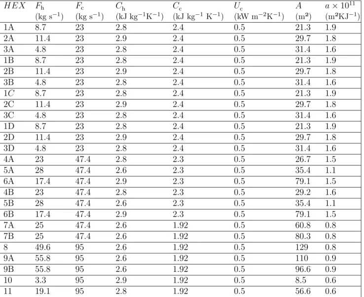
Table 5: Data for 25 unit HEN case. Adapted from Smaïli et al., 2002a. HEX Fh (kg s−1) Fc (kg s−1) Ch (kJ kg−1K−1) Cc (kJ kg−1 K−1) Uc (kW m−2K−1) A (m²) a×1011 (m²KJ−1) 1A 8.7 23 2.8 2.4 0.5 21.3 1.9 2A 11.4 23 2.9 2.4 0.5 29.7 1.8 3A 4.8 23 2.8 2.4 0.5 31.4 1.6 1B 8.7 23 2.8 2.4 0.5 21.3 1.9 2B 11.4 23 2.9 2.4 0.5 29.7 1.8 3B 4.8 23 2.8 2.4 0.5 31.4 1.6 1C 8.7 23 2.8 2.4 0.5 21.3 1.9 2C 11.4 23 2.9 2.4 0.5 29.7 1.8 3C 4.8 23 2.8 2.4 0.5 31.4 1.6 1D 8.7 23 2.8 2.4 0.5 21.3 1.9 2D 11.4 23 2.9 2.4 0.5 29.7 1.8 3D 4.8 23 2.8 2.4 0.5 31.4 1.6 4A 23 47.4 2.8 2.3 0.5 26.7 1.5 5A 28 47.4 2.6 2.3 0.5 35.4 1.1 6A 17.4 47.4 2.9 2.3 0.5 79.1 1.5 4B 23 47.4 2.8 2.3 0.5 29.2 1.6 5B 28 47.4 2.6 2.3 0.5 35.4 1.1 6B 17.4 47.4 2.9 2.3 0.5 79.1 1.5 7A 25 47.4 2.6 1.92 0.5 60.8 0.8 7B 25 47.4 2.6 1.92 0.5 80.3 0.8 8 49.6 95 2.6 1.92 0.5 129 0.8 9A 55.8 95 2.6 1.92 0.5 110 0.9 9B 55.8 95 2.6 1.92 0.5 96.6 0.9 10 3.3 95 2.9 1.92 0.5 8.5 0.6 11 19.1 95 2.8 1.92 0.5 56.6 0.6
T able 6: Op erational cons tr ain t for 25 unit HEN case. vacuum residue rundo wn temp erature target y1A,p + y1B ,p + y1C ,p + y1D ,p + y6A,p + y6B ,p ≥ 5 atmospheric middle pump-around target y2A,p + y2B ,p + y2C ,p + y2D ,p + y4A,p + y4B ,p ≥ 5 side-stream rundo wn temp erature target y3A,p + y3B ,p + y3C ,p + y3D ,p + y11 ,p ≥ 4 atmospheric top pump-around target y5A,p + y5B ,p + y9A,p + y9B ,p ≥ 3 vacuum pump-around target y7A,p + y7B ,p + y8,p ≥ 2 one hot end exc hanger is allo w ed to be cleaned at a time y1A,p + y2A,p + y3A,p ≥ 2 y1B ,p + y2B ,p + y3B ,p ≥ 2 y1C ,p + y2C ,p + y3C ,p ≥ 2 y1D ,p + y2D ,p + y3D ,p ≥ 2 flash temp erature is required to be main tained y4A,p + y5A,p + y6A,p ≥ 2 y4B ,p + y5B ,p + y6B ,p ≥ 2 main tenance of the desalter temp erature y7A,p + y7B ,p + y8,p + y9A,p + y9B ,p + y10 ,p + y11 ,p ≥ 6 temp erature dr op across desalter T in c,6p = T out c,7p − 10
fouling, where there is an insignificant difference in savings. This is because of the existence
339
of multiple local optima. It is noteworthy that Lavaja and Bagajewicz’s (2004) MILP model
340
is solved to global optimality whereas our model, being a non-convex MINLP model, is not.
341
Despite this, we still obtain similar results.
342
For the 10 unit HEN (tables 14 and 15), although a general relation is seen in Lavaja
343
and Bagajewicz’s schedule where cleaning actions increase in the asymptotic fouling case vs.
344
the linear one (from 10 to 11 cleanings), this drops down by 4 cleaning actions in our model
345
as shown in tables 14 and 15. Only the last 3 units are cleaned here whilst there is a more
346
distributed cleaning of units in the schedule of Lavaja and Bagajewicz, with half the units
347
in the network undergoing cleaning during the operational horizon. Consequently, the cost
348
of their schedule is slightly less than ours (£484k versus £493k as shown in table 9). This is
349
a small difference of just over 1.5% in savings.
350
For all reported schedules there is an absence of cleaning actions near the start and the end
351
of the operating horizon as there is little incentive to clean a relatively clean unit and there is
352
little time for the cost of cleaning to be recovered towards the end of the operating horizon.
353
If one were to increase the cost of cleaning further, this would limit the number of cleaning
354
actions even more and increase the objective further. This can be used to determine which
355
cleaning actions and/or exchangers are more important. For the 10 unit HEN, from tables
356
14 and 15, it can be seen that exchangers 9 and 10 are cleaned most frequently, indicating
357
that these exchangers are more important in the network, while exchangers 1 and 2 in the
358
linear and asymptotic models are not cleaned at all. Exchangers 9 and 10 are cleaned more
359
often as they have the highest fouling rates as shown in table 3. The fouling rate is not the
360
only criterion that determines how often cleaning is done. For instance as shown in table 3
361
in Lavaja and Bagajewicz’s (2004) schedule, despite the similar asymptotic fouling rates of
362
exchangers 5 and 7, the former is not cleaned at all while the latter is cleaned twice during
363
the operating horizon. This is due to network sensitivity.
364
An important point to note is the bang-bang nature of these problems. The solutions
of the relaxed models are completely integer i.e. a bang-bang control solution. Thus, the
366
proposed rounding up scheme was not performed here. A number of schedules with similar
367
objective values but different order of cleaning actions are obtained where very few fractional
368
binary variables occur. These solutions are termed bang-singular. For the majority of cases,
369
the range of objective values obtained in the 50 runs is quite narrow as shown in table 17,
370
where the objective values only vary from as little as £3k up to £15k in the first 5 case
371
studies. For the 10 unit asymptotic HEN case study, this range widens up to to £42k with a
372
minimum of £493k to a maximum of £535k, and up to £28k for the 25 unit HEN case study
373
with a variation of £902k to £930k. Hence, for less complex networks and/or fouling models
374
many runs at different starting points are not required to obtain a good solution.
375
A cost comparison only makes sense in the case studies appearing in Lavaja and
Baga-376
jewicz (2004) where the objective value for the no cleaning scenarios are similar (see tables
377
7 to 9). For the 25 unit HEN case studies, Smaïli et al. (2002a) reported a lower objective
378
associated with the no cleaning scenario representing <11% difference (see table 10). This is
379
partly attributed to our model retaining the fouling expressions in their dynamic form, which
380
is more accurate. Smaïli et al. (2002a) discretised the system equations and thus assumed
381
that variables such as temperature of hot and cold stream are fixed within each sub-period
382
which is not a good approximation for large complex networks with extensive feedback of
383
hot/cold streams. Temperatures in our model are interpreted continuously over time. The
384
difference in the objective for the no cleaning scenario in the 25 unit HEN is also attributed
385
to the different numerical methods used to the solve the equation sets.
386
For the 25 unit HEN case study our solution yields a saving of 36.2% with an overall
387
cost of £902k, whereas the best reported cost produced by Smaïli et al. (2002a) using their
388
BTA algorithm is £917k. Smaïli et al. (2002a) were unable to generate a solution using the
389
OA method. Our schedules have a small number of cleaning actions, in common with that
390
of Smaïli et al.. As in the 4 units over 18 months case study, no pattern is evident in the
391
cleaning actions for the Smaïli et al. (2002a) method. More cleaning actions are performed
in our schedule (37 versus 34, table 16). Some features in common are that most exchangers
393
are cleaned the same number of times as our schedule and certain exchangers are not cleaned
394
at all (e.g. exchanger 10).
395
In terms of the distribution of the objective values for the 50 runs performed in each case,
396
the results for each of the cases is narrowly dispersed around its associated mean value. The
397
relative standard deviation (RSD) of the local optima for each of the cases considered lies in
398
a narrow range of 0.8 to 1.5% (table 17). Furthermore, the difference between the maximum
399
and minimum cost value is only £3k for the 4 unit heat exchanger case over a 12 month
400
operating horizon, whereas this difference is the highest for the 10 unit HEN case subject to
401
asymptotic fouling, at £42k. For the 10 unit HEN case subject to asymptotic fouling, the
402
worst run results in a saving of 3.6% compared to 11.2% for the best solution achieved, while
403
for the 4 unit heat exchanger case over a 12 month length of operation this is a saving of
404
19.3% in the worst case compared to 21.5% in the best case scenario.
405
The resource usage varies depending on fouling type, method used and problem size.
406
Reasonable time for convergence is achieved for cases studies appearing in Lavaja and
Baga-407
jewicz (2004) and resource usage is practical even for the worst case: the 10 unit HEN with
408
asymptotic fouling model required 942 CPU s (15.7 CPU min), with the corresponding best
409
case for this model being a modest 91 CPU s. Lavaja and Bagajewicz (2004) stated that the
410
time to solve the 10 unit HEN case was impractical, therefore in addition to reformulating
411
their model into a MILP problem they used a decomposition procedure to decrease the
com-412
putational time. They also stated that they kept the linearity of the expressions with the
413
aim of having better chances of capturing the global optimum. From our findings, neither of
414
these are required. In comparison, the resource usage becomes expensive for the 25 unit HEN
415
case study. This required 55,243 CPU s (15.3 CPU hr) with 38,603 function evaluations in
416
the worst case. This is due to the implementation approach whereby gradients are estimated
417
using finite differences in the MATLAB® optimiser.
418
The computational cost is proportional to the number of finite difference calculations
required, with each finite difference calculation requiring a full dynamic system simulation;
420
for larger problems, this leads to a significant computational cost. For example, for the single
421
heat exchanger case under linear fouling for an operating horizon of 24 periods, an average of
422
11 gradient calculations is required with each one requiring 24 finite difference calculations,
423
as shown in Table 17. This accounts for the average computational cost of 30 CPU s. In
424
the case of the 25 unit heat exchanger network under linear fouling over 36 periods results
425
in a much larger average computational time of 39,611 CPU s (11 CPU hr). In this case,
426
there is an average of 31 gradient calculations each of them requiring 900 finite difference
427
calculations.
428
Future applications of the multistage optimal control approach will include the reduction
429
of CPU time such that it becomes significantly smaller in larger and more complex networks.
430
This will be achieved through gradient estimation using sensitivity equations. Furthermore,
431
future work will involve extending the range of case studies in HENs to include pressure
432
drop constraints, variable throughput, and optimisation of operating conditions such as the
433
consumption of utilities. This approach is not limited to HENs, and future work will focus
434
on the optimisation of general scheduling maintenance problems.
435
6. Critique
436
This work has demonstrated that the heat exchanger cleaning scheduling problem as
437
posed, considering all potential cleaning actions, can be solved for large networks and larger
438
numbers of actions than previously achieved through the recognition of the task as an optimal
439
control problem where the solutions fit bang-bang characteristics. We here review which
440
aspects of the scheduling problem which may be encountered in practice have been included
441
in the work, and those which have not, in order to identify the scope and potential for further
442
development.
443
Aspects which have been included are the distribution of heat duties within networks in
444
response to cleaning actions, and their evolution; linear and nonlinear (asymptotic) fouling
T able 7: Economic chart for the single heat exc hanger case. All v alues in k£. Case This w ork’s mo del La va ja and Baga jewicz’s (20 04) mo del This w ork’s solution (relaxed MIOCP) La va ja and Baga jewicz’s (2004) solution La va ja and Baga jewicz’s (2004) solution No cleaning, linear fouling 203 203 20 3 No cleaning, asymptotic fouling 317 317 316 Cleaning cost=£4k, linear fouling 103 (103*) 102 102 Cleaning cost=£4k, asym ptot ic fouling 226 (226*) 225 225 * relaxed MI OCP completely in teger i.e. feasible solution
T able 8: Economic chart for the four heat exc hangers case. All v alues in k£. Case This w ork’s mo del La va ja and Baga jewicz’s (2004) mo del This w ork’s
solution (relaxed MIOCP)
La va ja and Baga jewicz’s (2004) solution La va ja and Baga jewicz’s (2004) solution No cleaning, linear fouling, 12 mon th s 135 135 Not rep orted No cleaning, linear fouling, 18 mon th s 289 289 Not rep orted Cleaning cost = £4k, linear fouling, 12 mon ths 106 (106*) 106 106 Cleaning cost = £4k, linear fouling, 18 mon ths 179 (179*) 183 183 * relaxed MIO CP completely in teger i.e. feasible solution
T able 9: Economic chart for the 10 unit HEN cas e. All v alues in k£. Case This w ork’s mo del La va ja and Baga jewicz’s (2004) mo del
This work’s solution (relaxed MIOCP)
La va ja and Baga-jewicz’s (2004) solution La va ja and Baga jewicz’s (2004) solution No cleaning, linear fouling 361 361 361 No cleaning, asymptotic fouling 555 555 554 Cleaning cost = £4k, linear fo uling 259 (259*) 258 258 Cleaning cost = £4k, asymptotic foulin g 493 (493*) 48 4 48 2 * relaxed MI OCP completely in teger i.e. feasible solution
T able 10: Economic chart for the 25 unit HEN case . All v alues in k£. Case This w ork’s m odel Smaïli et al.’s (2002a) mo del This w ork’s solution (relaxed MIOCP) Smaïli et al.’s (2002a) O A metho d solu tion Smaïli et al.’s (2002a) BT A algorithm solution Smaïli et al.’s (2002a) O A metho d solution Smaïli et al.’s (2002a) BT A algorithm solution No cleaning, 36 mon ths 1413 1413 1413 Not rep orted 1261 Cleaning cost = £5k, 36 m on ths 902 (902*) Smaïli et al. unable to solv e 917 Smaïli et al. unable to solv e 819 * relaxed MI OCP completely in teger i.e. feasible solution
T able 11: Cleaning sc hedule for the single heat exc hanger case (line a r and asymptotic fouling). Case Time (mon ths) No. of cleaning actions 1 2 3 4 5 6 7 8 9 10 11 12 13 14 15 16 17 18 19 20 21 22 23 24 + , Linear fouling, cleaning cost=£4000 + , + , + , 3 3 Asymptotic fouling, cleaning cost=£4000 ⊕ ⊕ ⊕ , ⊕ ⊕ 5 6 cleaning actions: + this w ork; , La va ja and Baga jewicz; ⊕ common
T able 12: Cleaning sc hedule for the four heat exc hanger case (duration 12 mon ths, linear fouling, cleaning cost = £4000) Exc hanger No. Time (mon ths) No. of cleaning actions 1 2 3 4 5 6 7 8 9 10 11 12 + , 1 0 0 2 0 0 3 ⊕ 1 1 4 ⊕ 1 1 cleaning actions: + this w ork; , La va ja and Baga jewicz; ⊕ common 2 2
T able 13: Cleaning sc hedule for the four heat exc hanger case (duration 1 8 mon ths, linear fouling, cleaning cost = £4k) Exc hanger No. Time (mon ths) No. of cleaning actions 1 2 3 4 5 6 7 8 9 10 11 12 13 14 15 16 17 18 + , 1 + , 1 1 2 ⊕ 1 1 3 , + , + 2 2 4 ⊕ ⊕ 2 2 cleaning actions: + this w ork; , La va ja and Baga jewicz; ⊕ common 6 6
T able 14: Cleaning sc hedule for the 10 unit HEN case (linear fouling, cleaning cost = £4k). Exc hanger No. Time (mon ths) No. of cleaning actions 1 2 3 4 5 6 7 8 9 10 11 12 13 14 15 16 17 18 + , 1 0 0 2 0 0 3 ⊕ 1 1 4 ⊕ 1 1 5 , + 1 1 6 , + 1 1 7 + , 1 1 8 ⊕ 1 1 9 ⊕ ⊕ 2 2 10 ⊕ ⊕ 2 2 cleaning actions: + this w ork; , La va ja and Baga jewicz; ⊕ common 10 10
T able 15: Cleaning sc hedule for the 10 unit HEN case (asymptotic fouling, cleaning cost = £4k ). Exc hanger No. Time (mon ths) No. of cleaning actions 1 2 3 4 5 6 7 8 9 10 11 12 13 14 15 16 17 18 + , 1 0 0 2 0 0 3 0 0 4 , 0 1 5 0 0 6 0 0 7 , , 0 2 8 , + , 1 2 9 , + , + , 2 3 10 + , + , + , 3 3 cleaning actions: + this w ork; , La va ja and Baga jewicz; ⊕ common 6 11
T able 16: Cleaning sc hedule for the 25 unit HEN case (linear fouling, cleaning cost = £5k). H E X Time (mon ths) No. of cleaning actions 1 2 3 4 5 6 7 8 9 10 11 12 13 14 15 16 17 18 19 20 21 22 23 24 25 26 27 28 29 30 31 32 33 34 35 36 + , 1A , + + , 2 2 1B + , ⊕ 2 2 1C + , , + 2 2 1D , + , + 2 2 2A + , + , 2 2 2B + , ⊕ 2 2 2C , + , + 2 2 2D + , ⊕ 2 2 3A + 1 0 3B + 1 0 3C + , 1 1 3D , + 1 1 4A , + ⊕ 2 2 4B + , , + 2 2 5A + , 1 1 5B , + 1 1 6A , + , + 2 2 6B + , + 2 1 7A + , 1 1 7B + , 1 1 8 ⊕ 1 1 9A ⊕ 1 1 9B , + , + 2 2 10 0 0 11 , + 1 1 cleaning actions: + this w ork; , Smaïli et al. BT A algorithm; ⊕ common 37 34
T able 17: Solution metrics for all case studies. Case Study Ob jectiv e (i n k£) No. of iterations No. of function ev aluations ( i.e. sim ulations) CPU time (in s) Min Max Mean RSD (in %) Min Max Mean Min Max Mean Min Max Mean Single, lin ear fouling, 24 mon ths 103 109 105 1.3 5 18 11 145 467 286 15 48 30
Single, asymptotic fouling,
24 mon ths 226 241 233 1.4 2 15 7 72 388 192 9 47 25 4 units, linear fouling, 12 mon ths 106 109 107 0.9 5 12 8 270 592 404 22 48 34 4 units, linear fouling, 18 mon ths 179 189 182 1.1 11 22 15 835 1609 1141 97 190 132 10 unit HEN, linear fouling, 18 mon ths 259 270 264 1.0 9 25 16 1581 4322 2782 298 822 535 10 unit HEN, asymptotic fouling, 18 mon ths 493 535 512 1.5 2 19 7 343 3292 1298 91 942 343 25 unit HEN, linear fouling, 36 mon ths 902 930 915 0.8 25 43 31 21944 38603 28042 30670 55243 39611
behaviour; and constraints on the selection of combination of cleaning actions representing
446
pump-around targets, rundown temperature targets, flash temperature maintenance, etc.
447
Aspects presented by other workers which could be included without loss of generality, but
448
requiring more detailed modelling and therefore solution time, include the choice between
449
two cleaning actions (Pogiatzis et al., 2011) and temperature target constraints (e.g. desalter
450
temperature, see Ishiyama et al. (2010)).
451
Those not included can be grouped as follows:
452
(i) Nonlinearity arising from fouling phenomena. Fouling rates are known to depend
453
strongly on temperature, and will therefore vary in an exchanger over time as fouling changes
454
the temperature distribution within a network. This level of detailed modelling can be
455
incorporated in greedy (Ishiyama et al., 2009a) and genetic algorithm approaches (Rodriguez
456
and Smith, 2007), at the expense of ensuring global optimality, as well as in these total
457
horizon approaches.
458
(ii) Nonlinearity arising from network dynamics. Fouling deposits change the pressure
459
drop across a heat exchanger as well as its heat transfer performance. The network model
460
presented here assumes constant stream flow rates, but fouling in practice can give rise to flow
461
redistribution between parallel streams as well as throughput reduction as a result of pumping
462
limitations (Yeap et al., 2004; Ishiyama et al., 2008). Changes in flow rate affect both local
463
fouling rates and the objective function, and network models incorporating pressure drop and
464
throughput dynamics have been constructed. The relationship between fouling resistance,
465
pressure drop and throughput is not linear: depending on the network configuration, it can
466
feature a threshold followed by a quasi-parabolic region. The heat duty in the objective
467
function (equation (24)) then contains a product of two variables (F˙
c and CIT), and with an
468
appropriate formulation, this is amenable to this total horizon approach.
469
(iii) Uncertainty in fouling models and model parameters. Wilson et al. (2017) recently
470
reviewed the progress in quantitative fouling models for crude oil fouling. They reported
471
three areas where systematic uncertainty arise in models for predicting the fouling rates in
crude oil as related to the problems presented here:
473
(a) The fouling models are semi-empirical and the relationship to crude oil composition
474
and characteristics has yet to be established, so one cannot predict, for example, whether
475
linear or asymptotic fouling will be observed in a given unit.
476
(b) Fouling rates for complex fluids such as crude oil are rarely studied under controlled
477
conditions. In practice many operators used fouling models constructed from reconciliation
478
and interpretation of plant fouling data. These are subject to uncertainties in measurement
479
and calculation, so the accuracy of the fouling rate data is low.
480
(c) The relationship between fouling rates and crude composition is unknown. In most
481
applications the crude being processed varies with time so the rate(s) will also vary. This is
482
one of the reasons why plant fouling data, used to quantify fouling model parameters, contain
483
noticeable scatter and variation. These areas mean that, in practice, scheduling calculations
484
must be able to consider a range of likely fouling rates.
485
There is a conflict between aspects (i) and (ii), and (iii): the increased model complexity in
486
the former means that multiple condition testing, as required by (iii), will require considerable
487
resource. The desire to account for known, deterministic phenomena must be balanced
488
against the limitations to tractability introduced by those phenomena. From an engineering
489
perspective, the question to be asked is which essential features of the problem must be
490
included, at a suitable level of detail, to achieve the desired outcome.
491
Aspects (i) and (ii) will require special reformulation to be incorporated in a suitable level
492
of detail for some practical cases with total horizon approaches, such as the one described
493
in this work. These approaches are, however, ideally suited for combination with algorithms
494
for designing heat exchanger networks as they can generate estimates for expecting optimal
495
operating performance, including considerations of uncertainty in fouling (and operating
496
parameters).
497
For the case of a crude preheat train, the initial network design would yield temperature
498
and flow rate conditions for which fouling rates could be estimated. The operation of this
network, with cleaning schedules calculated for a portfolio of fouling rates, could then be
500
quantified (and key exchangers identified for design attention), and this information used
501
to update the design. Wang and Smith (2013) employed simulated annealing approaches
502
to identify fouling resistant preheat train designs but did not incorporate cleaning aspects
503
in their consideration of network performance: the current work now makes this a tractable
504
problem and one worthy of attention. Current network complexities may prohibit application
505
of a full optimisation based methodology for the scheduling of cleaning, and hence currently
506
the preference in industry is to use heuristic or greedy approaches. However, the contribution
507
of this work is to show that optimisation based methodologies can be general enough to
508
encapsulate both complexity and different operating modes and this will be explored further
509
in future work.
510
7. Conclusions
511
An alternative methodology to the solution of the HEN cleaning scheduling problem is
512
presented here by recognising, for the first time, that this optimisation model is in actuality
513
a MIOCP which exhibits bang-bang behaviour. This proves to be an efficient and robust
514
approach and has been compared with 3 different methods: a direct MINLP approach (OA),
515
reformulation of the MINLP to an MILP model, and a stochastic optimisation technique
516
(BTA algorithm).
517
The multistage optimal control formulation using the feasible path approach does not
518
suffer from failures in convergence and is thus reliable, contrary to the OA method which
519
fails to produce a solution in larger and more complex networks. The feasible path approach
520
as implemented is shown to be very competitive. Optimal solutions reported here are all
521
bang-bang in the controls. As a result, these particular case studies did not require any
522
heuristic approaches to be applied. In comparison to the classical methods, economic values
523
are similar and in some instances better than those obtained. The cleaning schedules showed
524
several conventional characteristics, with key exchangers being cleaned more often. However,
the allocation of cleaning actions was often not systematic, i.e. unpredictable. 526
Acknowledgements
527
Support of this research by the Ministry of Higher Education in the Sultanate of Oman
528
and Petroleum Development Oman (PDO) is gratefully acknowledged.
529
References
530
Belghith, S. F., Lamnabhi-Lagarrigue, F., Rosset, M. M., 1986. Algebraic and geometric
531
methods in nonlinear control theory. Vol. 29. Springer Netherlands, Dordrecht.
532
Bellman, R., Glicksberg, I., Gross, O., 1956. On the bang-bang control problem. Quaterly of
533
Applied Mathematics 14 (1), 11–18.
534
Blakemore, N., Aris, R., 1962. Studies in optimization-V. The bang-bang control of a batch
535
reactor. Chemical Engineering Science 17, 591–598.
536
Bryson, A. E., Ho, Y.-C., 1975. Applied optimal control: Optimization, estimation, and
537
control. Hemisphere Publishing Corporation, New York-Washington-Philadelphia-London.
538
Casado, E., 1990. Model optimizes exchanger cleaning. Hydrocarbon Processing 69 (8), 71–
539
76.
540
Fouskakis, D., Draper, D., 2002. Stochastic optimization: a review. International Statistical
541
Review 70 (3), 315–349.
542
Georgiadis, M. C., Papageorgiou, L. G., 2000. Optimal energy and cleaning management in
543
heat exchanger networks under fouling. Chemical Engineering Research and Design 78 (2),
544
168–179.
545
Gonçalves, C. D. O., Queiroz, E. M., Pessoa, F. L. P., Liporace, F. S., Oliveira, S. G., Costa,
546
A. L. H., 2014. Heuristic optimization of the cleaning schedule of crude preheat trains.
547
Applied Thermal Engineering 73 (1), 1–12.