Learning Deep Features for Discriminative Localization

Learning Deep Features for Discriminative Localization

Bolei Zhou, Aditya Khosla, Agata Lapedriza, Aude Oliva, Antonio Torralba

Computer Science and Artificial Intelligence Laboratory, MIT

{

bzhou,khosla,agata,oliva,torralba

}

@csail.mit.edu

Abstract

In this work, we revisit the global average pooling layer proposed in [13], and shed light on how it explicitly enables the convolutional neural network to have remarkable local-ization ability despite being trained on image-level labels. While this technique was previously proposed as a means for regularizing training, we find that it actually builds a generic localizable deep representation that can be applied to a variety of tasks. Despite the apparent simplicity of global average pooling, we are able to achieve 37.1% top-5 error for object localization on ILSVRC 2014, which is re-markably close to the 34.2% top-5 error achieved by a fully supervised CNN approach. We demonstrate that our net-work is able to localize the discriminative image regions on a variety of tasks despite not being trained for them.

1. Introduction

Recent work by Zhouet al[33] has shown that the

con-volutional units of various layers of concon-volutional neural networks (CNNs) actually behave as object detectors de-spite no supervision on the location of the object was pro-vided. Despite having this remarkable ability to localize objects in the convolutional layers, this ability is lost when fully-connected layers are used for classification. Recently some popular fully-convolutional neural networks such as the Network in Network (NIN) [13] and GoogLeNet [24] have been proposed to avoid the use of fully-connected lay-ers to minimize the number of parametlay-ers while maintain-ing high performance.

In order to achieve this, [13] usesglobal average

pool-ingwhich acts as a structural regularizer, preventing

over-fitting during training. In our experiments, we found that the advantages of this global average pooling layer extend beyond simply acting as a regularizer - In fact, with a little tweaking, the network can retain its remarkable localization ability until the final layer. This tweaking allows identifying easily the discriminative image regions in a single forward-pass for a wide variety of tasks, even those that the network was not originally trained for. As shown in Figure 1(a), a

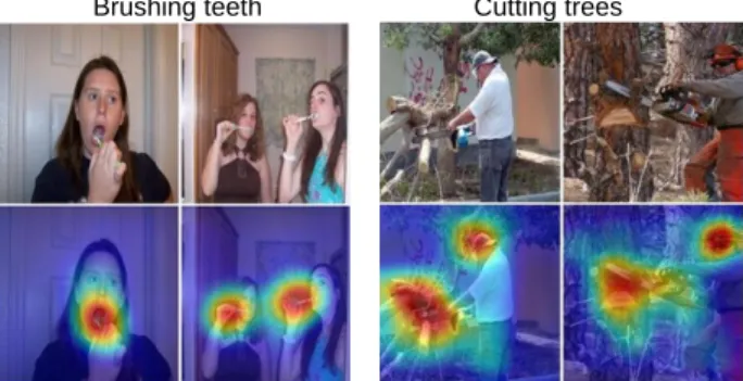
Brushing teeth Cutting trees

Figure 1. A simple modification of the global average pool-ing layer combined with our class activation mapppool-ing (CAM) technique allows the classification-trained CNN to both classify the image and localize class-specific image regions in a single

forward-pass e.g., the toothbrush forbrushing teethand the

chain-saw forcutting trees.

CNN trained on object categorization is successfully able to localize the discriminative regions for action classification as the objects that the humans are interacting with rather than the humans themselves.

Despite the apparent simplicity of our approach, for the weakly supervised object localization on ILSVRC bench-mark [20], our best network achieves 37.1% top-5 test er-ror, which is rather close to the 34.2% top-5 test error achieved by fully supervised AlexNet [10]. Furthermore, we demonstrate that the localizability of the deep features in our approach can be easily transferred to other recognition datasets for generic classification, localization, and concept

discovery.1_.

1.1. Related Work

Convolutional Neural Networks (CNNs) have led to im-pressive performance on a variety of visual recognition tasks [10, 34, 8]. Recent work has shown that despite being trained on image-level labels, CNNs have the remarkable ability to localize objects [1, 16, 2, 15]. In this work, we show that, using the right architecture, we can generalize this ability beyond just localizing objects, to start identi-fying exactly which regions of an image are being used for

1_{Our models are available at: http://cnnlocalization.csail.mit.edu}

discrimination. Here, we discuss the two lines of work most related to this paper: weakly-supervised object localization and visualizing the internal representation of CNNs.

Weakly-supervised object localization: There have

been a number of recent works exploring weakly-supervised object localization using CNNs [1, 16, 2, 15].

Bergamoet al[1] propose a technique for self-taught object

localization involving masking out image regions to iden-tify the regions causing the maximal activations in order to

localize objects. Cinbiset al[2] combine multiple-instance

learning with CNN features to localize objects. Oquab et

al[15] propose a method for transferring mid-level image

representations and show that some object localization can be achieved by evaluating the output of CNNs on multi-ple overlapping patches. However, the authors do not ac-tually evaluate the localization ability. On the other hand, while these approaches yield promising results, they are not trained end-to-end and require multiple forward passes of a network to localize objects, making them difficult to scale to real-world datasets. Our approach is trained end-to-end and can localize objects in a single forward pass.

The most similar approach to ours is the work based on

global max pooling by Oquabet al[16]. Instead of global

averagepooling, they apply globalmaxpooling to localize a point on objects. However, their localization is limited to a point lying in the boundary of the object rather than deter-mining the full extent of the object. We believe that while the maxand averagefunctions are rather similar, the use of average pooling encourages the network to identify the complete extent of the object. The basic intuition behind this is that the loss for average pooling benefits when the

network identifiesalldiscriminative regions of an object as

compared to max pooling. This is explained in greater de-tail and verified experimentally in Sec. 3.2. Furthermore, unlike [16], we demonstrate that this localization ability is generic and can be observed even for problems that the net-work was not trained on.

We useclass activation mapto refer to the weighted

acti-vation maps generated for each image, as described in Sec-tion 2. We would like to emphasize that while global aver-age pooling is not a novel technique that we propose here, the observation that it can be applied for accurate discrimi-native localization is, to the best of our knowledge, unique to our work. We believe that the simplicity of this tech-nique makes it portable and can be applied to a variety of computer vision tasks for fast and accurate localization.

Visualizing CNNs: There has been a number of recent

works [29, 14, 4, 33] that visualize the internal represen-tation learned by CNNs in an attempt to better understand

their properties. Zeileret al [29] use deconvolutional

net-works to visualize what patterns activate each unit. Zhouet

al.[33] show that CNNs learn object detectors while being

trained to recognize scenes, and demonstrate that the same

network can perform both scene recognition and object lo-calization in a single forward-pass. Both of these works only analyze the convolutional layers, ignoring the fully-connected thereby painting an incomplete picture of the full story. By removing the fully-connected layers and retain-ing most of the performance, we are able to understand our network from the beginning to the end.

Mahendranet al[14] and Dosovitskiyet al[4] analyze

the visual encoding of CNNs by inverting deep features at different layers. While these approaches can invert the fully-connected layers, they only show what information is being preserved in the deep features without highlight-ing the relative importance of this information. Unlike [14] and [4], our approach can highlight exactly which regions of an image are important for discrimination. Overall, our approach provides another glimpse into the soul of CNNs.

2. Class Activation Mapping

In this section, we describe the procedure for generating

class activation maps(CAM) using global average pooling (GAP) in CNNs. A class activation map for a particular cat-egory indicates the discriminative image regions used by the CNN to identify that category (e.g., Fig. 3). The procedure for generating these maps is illustrated in Fig. 2.

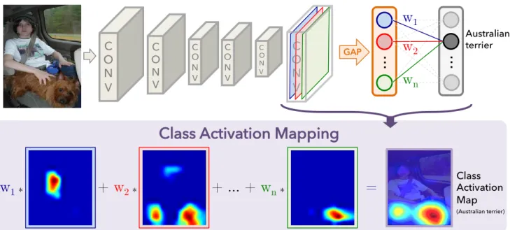
We use a network architecture similar to Network in Net-work [13] and GoogLeNet [24] - the netNet-work largely con-sists of convolutional layers, and just before the final out-put layer (softmax in the case of categorization), we per-form global average pooling on the convolutional feature maps and use those as features for a fully-connected layer that produces the desired output (categorical or otherwise). Given this simple connectivity structure, we can identify the importance of the image regions by projecting back the weights of the output layer on to the convolutional feature maps, a technique we call class activation mapping.

As illustrated in Fig. 2, global average pooling outputs the spatial average of the feature map of each unit at the last convolutional layer. A weighted sum of these values is used to generate the final output. Similarly, we compute a weighted sum of the feature maps of the last convolutional layer to obtain our class activation maps. We describe this more formally below for the case of softmax. The same technique can be applied to regression and other losses.

For a given image, letfk(x, y)represent the activation

of unitkin the last convolutional layer at spatial location

(x, y). Then, for unit k, the result of performing global

average pooling, Fk _is P

x,yfk(x, y). Thus, for a given

classc, the input to the softmax,Sc, isPkw

c

kFkwherewkc

is the weight corresponding to classcfor unitk. Essentially,

wc

k indicates theimportanceofFk for classc. Finally the

output of the softmax for classc,Pcis given byPexp(Sc)

cexp(Sc).

Australian terrier

...

C

O

N

V

...

w

w

w

w

+

w

+ … +

w

=

C

O

N

V

Class Activation Mapping

Figure 2. Class Activation Mapping: the predicted class score is mapped back to the previous convolutional layer to generate the class activation maps (CAMs). The CAM highlights the class-specific discriminative regions.

bias of the softmax to0as it has little to no impact on the

classification performance.

By pluggingFk = Px,yfk(x, y)into the class score,

Sc, we obtain Sc= X k wc_kX x,y fk(x, y) =X x,y X k w_kcfk(x, y). (1)

We defineMcas the class activation map for classc, where

each spatial element is given by

Mc(x, y) =

X

k

wc_kfk(x, y). (2)

Thus, Sc = Px,yMc(x, y), and henceMc(x, y)directly

indicates the importance of the activation at spatial grid

(x, y)leading to the classification of an image to classc. Intuitively, based on prior works [33, 29], we expect each unit to be activated by some visual pattern within its

recep-tive field. Thusfk is the map of the presence of this visual

pattern. The class activation map is simply a weighted lin-ear sum of the presence of these visual patterns at different spatial locations. By simply upsampling the class activa-tion map to the size of the input image, we can identify the image regions most relevant to the particular category.

In Fig. 3, we show some examples of the CAMs output using the above approach. We can see that the discrimi-native regions of the images for various classes are high-lighted. In Fig. 4 we highlight the differences in the CAMs

for a single image when using different classescto

gener-ate the maps. We observe that the discriminative regions

Figure 3. The CAMs of four classes from ILSVRC [20]. The maps highlight the discriminative image regions used for image

classifi-cation e.g., the head of the animal forbriardandhen, the plates in

barbell, and the bell inbell cote.

for different categories are different even for a given im-age. This suggests that our approach works as expected. We demonstrate this quantitatively in the sections ahead.

Global average pooling (GAP) vs global max

pool-ing (GMP):Given the prior work [16] on using GMP for

weakly supervised object localization, we believe it is im-portant to highlight the intuitive difference between GAP and GMP. We believe that GAP loss encourages the net-work to identify the extent of the object as compared to GMP which encourages it to identify just one discrimina-tive part. This is because, when doing the average of a map,

the value can be maximized by finding all discriminative

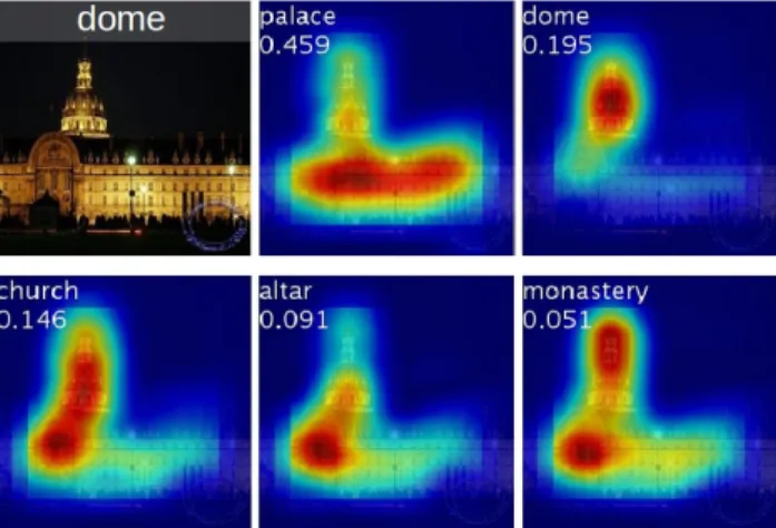
dome

chain saw

Figure 4. Examples of the CAMs generated from the top 5 pre-dicted categories for the given image with ground-truth as dome. The predicted class and its score are shown above each class ac-tivation map. We observe that the highlighted regions vary across

predicted classes e.g.,domeactivates the upper round part while

palaceactivates the lower flat part of the compound.

the particular map. On the other hand, for GMP, low scores for all image regions except the most discriminative one do not impact the score as you just perform a max. We ver-ify this experimentally on ILSVRC dataset in Sec. 3: while GMP achieves similar classification performance as GAP, GAP outperforms GMP for localization.

3. Weakly-supervised Object Localization

In this section, we evaluate the localization ability of CAM when trained on the ILSVRC 2014 benchmark dataset [20]. We first describe the experimental setup and the various CNNs used in Sec. 3.1. Then, in Sec. 3.2 we ver-ify that our technique does not adversely impact the classi-fication performance when learning to localize and provide detailed results on weakly-supervised object localization.

3.1. Setup

For our experiments we evaluate the effect of using CAM on the following popular CNNs: AlexNet [10], VG-Gnet [23], and GoogLeNet [24]. In general, for each of these networks we remove the fully-connected layers be-fore the final output and replace them with GAP followed by a fully-connected softmax layer.

We found that the localization ability of the networks im-proved when the last convolutional layer before GAP had a

higher spatial resolution, which we term themapping

reso-lution. In order to do this, we removed several convolutional layers from some of the networks. Specifically, we made the following modifications: For AlexNet, we removed the

layers after conv5(i.e., pool5 toprob) resulting in a

mapping resolution of13×13. For VGGnet, we removed

the layers after conv5-3(i.e., pool5toprob),

result-ing in a mappresult-ing resolution of14×14. For GoogLeNet,

we removed the layers afterinception4e(i.e.,pool4

to prob), resulting in a mapping resolution of 14×14.

To each of the above networks, we added a convolutional

layer of size3×3, stride1, pad1with 1024 units, followed

by a GAP layer and a softmax layer. Each of these

net-works were then fine-tuned2 _{on the 1.3M training images}

of ILSVRC [20] for 1000-way object classification result-ing in our final networks AlexNet-GAP, VGGnet-GAP and GoogLeNet-GAP respectively.

For classification, we compare our approach against the original AlexNet [10], VGGnet [23], and GoogLeNet [24], and also provide results for Network in Network (NIN) [13]. For localization, we compare against the

orig-inal GoogLeNet3_{, NIN and using backpropagation [22]}

instead of CAMs. Further, to compare average pooling

against max pooling, we also provide results for GoogLeNet trained using global max pooling (GoogLeNet-GMP).

We use the same error metrics (top-1, top-5) as ILSVRC for both classification and localization to evaluate our net-works. For classification, we evaluate on the ILSVRC vali-dation set, and for localization we evaluate on both the val-idation and test sets.

3.2. Results

We first report results on object classification to demon-strate that our approach does not significantly hurt classi-fication performance. Then we demonstrate that our ap-proach is effective at weakly-supervised object localization.

Classification:Tbl. 1 summarizes the classification

per-formance of both the original and our GAP networks. We find that in most cases there is a small performance drop

of 1−2% when removing the additional layers from the

various networks. We observe that AlexNet is the most affected by the removal of the fully-connected layers. To compensate, we add two convolutional layers just before GAP resulting in the AlexNet*-GAP network. We find that AlexNet*-GAP performs comparably to AlexNet. Thus, overall we find that the classification performance is largely preserved for our GAP networks. Further, we observe that GoogLeNet-GAP and GoogLeNet-GMP have similar per-formance on classification, as expected. Note that it is im-portant for the networks to perform well on classification in order to achieve a high performance on localization as it involves identifying both the object category and the bound-ing box location accurately.

Localization:In order to perform localization, we need

to generate a bounding box and its associated object cate-gory. To generate a bounding box from the CAMs, we use a simple thresholding technique to segment the heatmap. We first segment the regions of which the value is above 20%

2_{Training from scratch also resulted in similar performances.} 3_{This has a lower mapping resolution than GoogLeNet-GAP.}

Table 1. Classification error on the ILSVRC validation set.

Networks top-1 val. error top-5 val. error

VGGnet-GAP 33.4 12.2 GoogLeNet-GAP 35.0 13.2 AlexNet∗_{-GAP 44.9 20.9} AlexNet-GAP 51.1 26.3 GoogLeNet 31.9 11.3 VGGnet 31.2 11.4 AlexNet 42.6 19.5 NIN 41.9 19.6 GoogLeNet-GMP 35.6 13.9

of the max value of the CAM. Then we take the bounding box that covers the largest connected component in the seg-mentation map. We do this for each of the top-5 predicted classes for the top-5 localization evaluation metric. Fig. 6(a) shows some example bounding boxes generated using this technique. The localization performance on the ILSVRC validation set is shown in Tbl. 2, and example outputs in Fig. 5.

We observe that our GAP networks outperform all the baseline approaches with GoogLeNet-GAP achieving the

lowest localization error of43%on top-5. This is

remark-able given that this network was not trained on a single annotated bounding box. We observe that our CAM proach significantly outperforms the backpropagation ap-proach of [22] (see Fig. 6(b) for a comparison of the out-puts). Further, we observe that GoogLeNet-GAP signifi-cantly outperforms GoogLeNet on localization, despite this being reversed for classification. We believe that the low

mapping resolution of GoogLeNet (7×7) prevents it from

obtaining accurate localizations. Last, we observe that

GoogLeNet-GAP outperforms GoogLeNet-GMP by a rea-sonable margin illustrating the importance of average pool-ing over max poolpool-ing for identifypool-ing the extent of objects.

To further compare our approach with the existing weakly-supervised [22] and fully-supervised [24, 21, 24] CNN methods, we evaluate the performance of GoogLeNet-GAP on the ILSVRC test set. We follow a slightly differ-ent bounding box selection strategy here: we select two bounding boxes (one tight and one loose) from the class activation map of the top 1st and 2nd predicted classes and one loose bounding boxes from the top 3rd predicted class. We found that this heuristic was helpful to improve performances on the validation set. The performances are summarized in Tbl. 3. GoogLeNet-GAP with heuristics achieves a top-5 error rate of 37.1% in a weakly-supervised setting, which is surprisingly close to the top-5 error rate of AlexNet (34.2%) in a fully-supervised setting. While impressive, we still have a long way to go when com-paring the fully-supervised networks with the same archi-tecture (i.e., weakly-supervised GoogLeNet-GAP vs fully-supervised GoogLeNet) for the localization.

Table 2. Localization error on the ILSVRC validation set.

Back-proprefers to using [22] for localization instead of CAM.

Method top-1 val.error top-5 val. error GoogLeNet-GAP 56.40 43.00 VGGnet-GAP 57.20 45.14 GoogLeNet 60.09 49.34 AlexNet∗-GAP 63.75 49.53 AlexNet-GAP 67.19 52.16 NIN 65.47 54.19 Backprop on GoogLeNet 61.31 50.55 Backprop on VGGnet 61.12 51.46 Backprop on AlexNet 65.17 52.64 GoogLeNet-GMP 57.78 45.26

Table 3. Localization error on the ILSVRC test set for various weakly- and fully- supervised methods.

Method supervision top-5 test error GoogLeNet-GAP (heuristics) weakly 37.1

GoogLeNet-GAP weakly 42.9

Backprop [22] weakly 46.4

GoogLeNet [24] full 26.7

OverFeat [21] full 29.9

AlexNet [24] full 34.2

4. Deep Features for Generic Localization

The responses from the higher-level layers of CNN (e.g.,

fc6,fc7from AlexNet) have been shown to be very

effec-tive generic features with state-of-the-art performance on a variety of image datasets [3, 19, 34]. Here, we show that the features learned by our GAP CNNs also perform well as generic features, and as bonus, identify the discrimina-tive image regions used for categorization, despite not hav-ing behav-ing trained for those particular tasks. To obtain the weights similar to the original softmax layer, we simply train a linear SVM [5] on the output of the GAP layer.

First, we compare the performance of our approach and some baselines on the following scene and ob-ject classification benchmarks: SUN397 [27], MIT In-door67 [18], Scene15 [11], SUN Attribute [17], Cal-tech101 [6], Caltech256 [9], Stanford Action40 [28], and UIUC Event8 [12]. The experimental setup is the same as in [34]. In Tbl. 5, we compare the performance of features

from our best network, GoogLeNet-GAP, with thefc7

fea-tures from AlexNet, andave poolfrom GoogLeNet.

As expected, GoogLeNet-GAP and GoogLeNet

sig-nificantly outperform AlexNet. Also, we observe that

GoogLeNet-GAP and GoogLeNet perform similarly de-spite the former having fewer convolutional layers. Overall, we find that GoogLeNet-GAP features are competitive with the state-of-the-art as generic visual features.

More importantly, we want to explore whether the lo-calization maps generated using our CAM technique with GoogLeNet-GAP are informative even in this scenario. Fig. 8 shows some example maps for various datasets. We observe that the most discriminative regions tend to be high-lighted across all datasets. Overall, our approach is effective

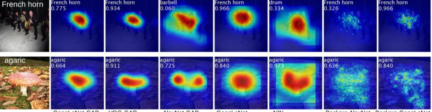
GoogLeNet-GAP VGG-GAP AlexNet-GAP GoogLeNet NIN Backpro AlexNet Backpro GoogLeNet

agaric French horn

Figure 5. Class activation maps from CNN-GAPs and the class-specific saliency map from the backpropagation methods.

b) a)

Figure 6. a) Examples of localization from GoogleNet-GAP. b) Comparison of the localization from GooleNet-GAP (upper two) and the backpropagation using AlexNet (lower two). The ground-truth boxes are in green and the predicted bounding boxes from the class activation map are in red.

for generating localizable deep features for generic tasks. In Sec. 4.1, we explore fine-grained recognition of birds and demonstrate how we evaluate the generic localiza-tion ability and use it to further improve performance. In Sec. 4.2 we demonstrate how GoogLeNet-GAP can be used to identify generic visual patterns from images.

4.1. Fine-grained Recognition

In this section, we apply our generic localizable deep features to identifying 200 bird species in the CUB-200-2011 [26] dataset. The dataset contains 11,788 images, with 5,994 images for training and 5,794 for test. We choose this dataset as it also contains bounding box annotations allow-ing us to evaluate our localization ability. Tbl. 4 summarizes the results.

We find that GoogLeNet-GAP performs comparably to existing approaches, achieving an accuracy of 63.0% when using the full image without any bounding box annotations for both train and test. When using bounding box anno-tations, this accuracy increases to 70.5%. Now, given the localization ability of our network, we can use a similar ap-proach as Sec. 3.2 (i.e., thresholding) to first identify bird bounding boxes in both the train and test sets. We then use GoogLeNet-GAP to extract features again from the crops inside the bounding box, for training and testing. We find that this improves the performance considerably to 67.8%.

Table 4. Fine-grained classification performance on CUB200 dataset. GoogLeNet-GAP can successfully localize important im-age crops, boosting classification performance.

Methods Train/Test Anno. Accuracy GoogLeNet-GAP on full image n/a 63.0% GoogLeNet-GAP on crop n/a 67.8% GoogLeNet-GAP on BBox BBox 70.5%

Alignments [7] n/a 53.6%

Alignments [7] BBox 67.0%

DPD [31] BBox+Parts 51.0%

DeCAF+DPD [3] BBox+Parts 65.0% PANDA R-CNN [30] BBox+Parts 76.4%

This localization ability is particularly important for fine-grained recognition as the distinctions between the cate-gories are subtle and having a more focused image crop allows for better discrimination.

Further, we find that GoogLeNet-GAP is able to accu-rately localize the bird in 41.0% of the images under the 0.5 intersection over union (IoU) criterion, as compared to a chance performance of 5.5%. We visualize some exam-ples in Fig. 7. This further validates the localization ability of our approach.

4.2. Pattern Discovery

In this section, we explore whether our technique can identify common elements or patterns in images beyond

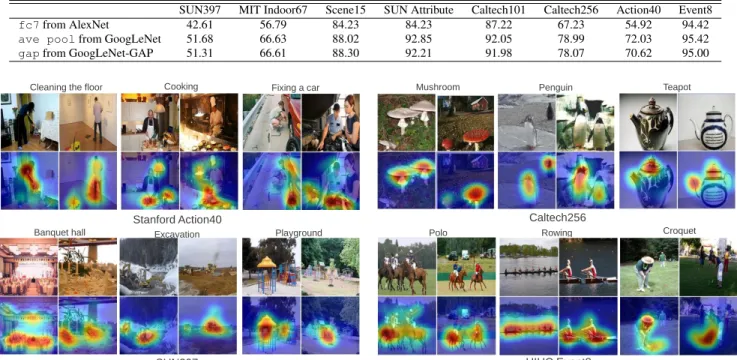
Table 5. Classification accuracy on representative scene and object datasets for different deep features.

SUN397 MIT Indoor67 Scene15 SUN Attribute Caltech101 Caltech256 Action40 Event8 fc7from AlexNet 42.61 56.79 84.23 84.23 87.22 67.23 54.92 94.42 ave poolfrom GoogLeNet 51.68 66.63 88.02 92.85 92.05 78.99 72.03 95.42 gapfrom GoogLeNet-GAP 51.31 66.61 88.30 92.21 91.98 78.07 70.62 95.00

Fixing a car

Cleaning the floor Cooking Mushroom Penguin Teapot

Stanford Action40 Caltech256

Rowing Polo UIUC Event8 Croquet Playground SUN397 Excavation Banquet hall

Figure 8. Generic discriminative localization using our GoogLeNet-GAP deep features (which have been trained to recognize objects). We show 2 images each from 3 classes for 4 datasets, and their class activation maps below them. We observe that the discriminative regions

of the images are often highlighted e.g., in Stanford Action40, the mop is localized forcleaning the floor, while forcookingthe pan and

bowl are localized and similar observations can be made in other datasets. This demonstrates the generic localization ability of our deep features.

White Pelican

Orchard Oriole Sage Thrasher

Scissor tailed Flycatcher

Figure 7. CAMs and the inferred bounding boxes (in red) for se-lected images from four bird categories in CUB200. In Sec. 4.1 we quantitatively evaluate the quality of the bounding boxes (41.0% accuracy for 0.5 IoU). We find that extracting GoogLeNet-GAP features in these CAM bounding boxes and re-training the SVM improves bird classification accuracy by about 5% (Tbl. 4).

objects, such as text or high-level concepts. Given a set of images containing a common concept, we want to iden-tify which regions our network recognizes as being impor-tant and if this corresponds to the input pattern. We

fol-low a similar approach as before: we train a linear SVM on the GAP layer of the GoogLeNet-GAP network and apply the CAM technique to identify important regions. We con-ducted three pattern discovery experiments using our deep features. The results are summarized below. Note that in

this case, we do not have train and test splits−we just use

our CNN for visual pattern discovery.

Discovering informative objects in the scenes: We

take 10 scene categories from the SUN dataset [27]

contain-ing at least200fully annotated images, resulting in a total

of 4675 fully annotated images. We train a one-vs-all linear SVM for each scene category and compute the CAMs using the weights of the linear SVM. In Fig. 9 we plot the CAM for the predicted scene category and list the top 6 objects that most frequently overlap with the high CAM activation regions for two scene categories. We observe that the high activation regions frequently correspond to objects indica-tive of the particular scene category.

Concept localization in weakly labeled images:

Us-ing the hard-negative minUs-ing algorithm from [32], we learn concept detectors and apply our CAM technique to local-ize concepts in the image. To train a concept detector for a short phrase, the positive set consists of images that con-tain the short phrase in their text caption, and the negative set is composed of randomly selected images without any relevant words in their text caption. In Fig. 10, we visualize

Informative object: sink:0.84 faucet:0.80 countertop:0.80 toilet:0.72 bathtub:0.70 towel:0.54 Informative object: table:0.96 chair:0.85 chandelier:0.80 plate:0.73 vase:0.69 flowers:0.63

Dining room Bathroom

Frequent object: wall:0.99 chair:0.98 floor:0.98 table:0.98 ceiling:0.75 window:73 Frequent object: wall: 1 floor:0.85 sink: 0.77 faucet:0.74 mirror:0.62 bathtub:0.56

Figure 9. Informative objects for two scene categories. For the din-ing room and bathroom categories, we show examples of original

images (top), and list of the6most frequent objects in that scene

category with the corresponding frequency of appearance. At the bottom: the CAMs and a list of the 6 objects that most frequently overlap with the high activation regions.

mirror in lake view out of window

Figure 10. Informative regions for the concept learned from weakly labeled images. Despite being fairly abstract, the concepts are adequately localized by our GoogLeNet-GAP network.

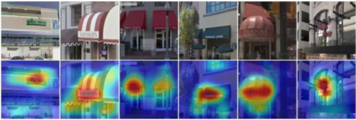
Figure 11. Learning a weakly supervised text detector. The text is accurately detected on the image even though our network is not trained with text or any bounding box annotations.

the top ranked images and CAMs for two concept detec-tors. Note that CAM localizes the informative regions for the concepts, even though the phrases are much more ab-stract than typical object names.

Weakly supervised text detector:We train a weakly

su-pervised text detector using 350 Google StreetView images containing text from the SVT dataset [25] as the positive set and randomly sampled images from outdoor scene images in the SUN dataset [27] as the negative set. As shown in Fig. 11, our approach highlights the text accurately without using bounding box annotations.

Interpreting visual question answering: We use our

approach and localizable deep feature in the baseline pro-posed in [35] for visual question answering. It has overall accuracy 55.89% on the test-standard in the Open-Ended track. As shown in Fig. 12, our approach highlights the im-age regions relevant to the predicted answers.

What is the color of the horse?

Prediction: brown What are they doing?Prediction: texting

What is the sport? Prediction: skateboarding

Where are the cows? Prediction: on the grass

Figure 12. Examples of highlighted image regions for the pre-dicted answer class in the visual question answering.

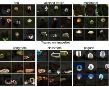
5. Visualizing Class-Specific Units

Zhouet al[33] have shown that the convolutional units of various layers of CNNs act as visual concept detec-tors, identifying low-level concepts like textures or mate-rials, to high-level concepts like objects or scenes. Deeper into the network, the units become increasingly discrimi-native. However, given the fully-connected layers in many networks, it can be difficult to identify the importance of different units for identifying different categories. Here, us-ing GAP and the ranked softmax weight, we can directly visualize the units that are most discriminative for a given

class. Here we call them theclass-specific unitsof a CNN.

Fig. 13 shows the class-specific units for AlexNet∗-GAP

trained on ILSVRC dataset for object recognition (top) and Places Database for scene recognition (bottom). We follow a similar procedure as [33] for estimating the receptive field and segmenting the top activation images of each unit in the final convolutional layer. Then we simply use the softmax weights to rank the units for a given class. From the figure we can identify the parts of the object that are most dis-criminative for classification and exactly which units detect these parts. For example, the units detecting dog face and

body fur are important tolakeland terrier; the units

detect-ing sofa, table and fireplace are important to theliving room.

Thus we could infer that the CNN actually learns a bag of words, where each word is a discriminative class-specific unit. A combination of these class-specific units guides the CNN in classifying each image.

6. Conclusion

In this work we propose a general technique called Class Activation Mapping (CAM) for CNNs with global average pooling. This enables classification-trained CNNs to learn to perform object localization, without using any bounding box annotations. Class activation maps allow us to visualize the predicted class scores on any given image, highlighting the discriminative object parts detected by the CNN. We evaluate our approach on weakly supervised object local-ization on the ILSVRC benchmark, demonstrating that our global average pooling CNNs can perform accurate object

pagoda classroom

livingroom

Trained on Places Database Trained on ImageNet

hen lakeland terrier mushroom

Figure 13. Visualization of the class-specific units for AlexNet*-GAP trained on ImageNet (top) and Places (bottom) respectively. The top 3 units for three selected classes are shown for each dataset. Each row shows the most confident images segmented by the receptive field of that unit. For example, units detecting blackboard, chairs, and tables are important to the classification of

classroomfor the network trained for scene recognition.

localization. Furthermore we demonstrate that the CAM lo-calization technique generalizes to other visual recognition tasks i.e., our technique produces generic localizable deep features that can aid other researchers in understanding the basis of discrimination used by CNNs for their tasks.

References

[1] A. Bergamo, L. Bazzani, D. Anguelov, and L. Torresani.

Self-taught object localization with deep networks. arXiv

preprint arXiv:1409.3964, 2014.

[2] R. G. Cinbis, J. Verbeek, and C. Schmid. Weakly supervised object localization with multi-fold multiple instance learn-ing. IEEE Trans. on Pattern Analysis and Machine Intelli-gence, 2015.

[3] J. Donahue, Y. Jia, O. Vinyals, J. Hoffman, N. Zhang, E. Tzeng, and T. Darrell. Decaf: A deep convolutional

ac-tivation feature for generic visual recognition. International

Conference on Machine Learning, 2014.

[4] A. Dosovitskiy and T. Brox. Inverting convolutional

networks with convolutional networks. arXiv preprint

arXiv:1506.02753, 2015.

[5] R.-E. Fan, K.-W. Chang, C.-J. Hsieh, X.-R. Wang, and C.-J.

Lin. Liblinear: A library for large linear classification. The

Journal of Machine Learning Research, 2008.

[6] L. Fei-Fei, R. Fergus, and P. Perona. Learning generative visual models from few training examples: An incremental

bayesian approach tested on 101 object categories.Computer

Vision and Image Understanding, 2007.

[7] E. Gavves, B. Fernando, C. G. Snoek, A. W. Smeulders, and T. Tuytelaars. Local alignments for fine-grained

categoriza-tion.Int’l Journal of Computer Vision, 2014.

[8] R. Girshick, J. Donahue, T. Darrell, and J. Malik. Rich fea-ture hierarchies for accurate object detection and semantic

segmentation.Proc. CVPR, 2014.

[9] G. Griffin, A. Holub, and P. Perona. Caltech-256 object cat-egory dataset. 2007.

[10] A. Krizhevsky, I. Sutskever, and G. E. Hinton. Imagenet

classification with deep convolutional neural networks. In

Advances in Neural Information Processing Systems, 2012.

[11] S. Lazebnik, C. Schmid, and J. Ponce. Beyond bags of

features: Spatial pyramid matching for recognizing natural

scene categories.Proc. CVPR, 2006.

[12] L.-J. Li and L. Fei-Fei. What, where and who? classifying

events by scene and object recognition.Proc. ICCV, 2007.

[13] M. Lin, Q. Chen, and S. Yan. Network in network.

Interna-tional Conference on Learning Representations, 2014. [14] A. Mahendran and A. Vedaldi. Understanding deep image

representations by inverting them.Proc. CVPR, 2015.

[15] M. Oquab, L. Bottou, I. Laptev, and J. Sivic. Learning and transferring mid-level image representations using

convolu-tional neural networks.Proc. CVPR, 2014.

[16] M. Oquab, L. Bottou, I. Laptev, and J. Sivic. Is object local-ization for free? weakly-supervised learning with

convolu-tional neural networks.Proc. CVPR, 2015.

[17] G. Patterson and J. Hays. Sun attribute database:

Discov-ering, annotating, and recognizing scene attributes. Proc.

CVPR, 2012.

[18] A. Quattoni and A. Torralba. Recognizing indoor scenes.

Proc. CVPR, 2009.

[19] A. S. Razavian, H. Azizpour, J. Sullivan, and S. Carlsson. Cnn features off-the-shelf: an astounding baseline for

recog-nition.arXiv preprint arXiv:1403.6382, 2014.

[20] O. Russakovsky, J. Deng, H. Su, J. Krause, S. Satheesh, S. Ma, Z. Huang, A. Karpathy, A. Khosla, M. Bernstein, A. C. Berg, and L. Fei-Fei. Imagenet large scale visual

recog-nition challenge. InInt’l Journal of Computer Vision, 2015.

[21] P. Sermanet, D. Eigen, X. Zhang, M. Mathieu, R. Fergus, and Y. LeCun. Overfeat: Integrated recognition, localization

and detection using convolutional networks. arXiv preprint

arXiv:1312.6229, 2013.

[22] K. Simonyan, A. Vedaldi, and A. Zisserman. Deep

in-side convolutional networks: Visualising image

classifica-tion models and saliency maps.International Conference on

Learning Representations Workshop, 2014.

[23] K. Simonyan and A. Zisserman. Very deep convolutional

networks for large-scale image recognition. International

Conference on Learning Representations, 2015.

[24] C. Szegedy, W. Liu, Y. Jia, P. Sermanet, S. Reed, D. Anguelov, D. Erhan, V. Vanhoucke, and A.

Rabi-novich. Going deeper with convolutions. arXiv preprint

arXiv:1409.4842, 2014.

[25] K. Wang, B. Babenko, and S. Belongie. End-to-end scene

text recognition.Proc. ICCV, 2011.

[26] P. Welinder, S. Branson, T. Mita, C. Wah, F. Schroff, S. Be-longie, and P. Perona. Caltech-UCSD Birds 200. Technical report, California Institute of Technology, 2010.

[27] J. Xiao, J. Hays, K. A. Ehinger, A. Oliva, and A. Torralba. Sun database: Large-scale scene recognition from abbey to zoo.Proc. CVPR, 2010.

[28] B. Yao, X. Jiang, A. Khosla, A. L. Lin, L. Guibas, and L. Fei-Fei. Human action recognition by learning bases of action

attributes and parts.Proc. ICCV, 2011.

[29] M. D. Zeiler and R. Fergus. Visualizing and understanding

convolutional networks.Proc. ECCV, 2014.

[30] N. Zhang, J. Donahue, R. Girshick, and T. Darrell.

Part-based r-cnns for fine-grained category detection. Proc.

ECCV, 2014.

[31] N. Zhang, R. Farrell, F. Iandola, and T. Darrell. Deformable part descriptors for fine-grained recognition and attribute

prediction.Proc. ICCV, 2013.

[32] B. Zhou, V. Jagadeesh, and R. Piramuthu. Conceptlearner: Discovering visual concepts from weakly labeled image

col-lections.Proc. CVPR, 2015.

[33] B. Zhou, A. Khosla, A. Lapedriza, A. Oliva, and A. Torralba.

Object detectors emerge in deep scene cnns. International

Conference on Learning Representations, 2015.

[34] B. Zhou, A. Lapedriza, J. Xiao, A. Torralba, and A. Oliva. Learning deep features for scene recognition using places

database.In Advances in Neural Information Processing

Sys-tems, 2014.

[35] B. Zhou, Y. Tian, S. Sukhbaatar, A. Szlam, and R.

Fer-gus. Simple baseline for visual question answering. arXiv