Mixing Linear SVMs for Nonlinear Classification
Zhouyu Fu, Antonio Robles-Kelly, Senior Member, IEEE, and Jun Zhou, Member, IEEE
Abstract— In this paper, we address the problem of combining
linear support vector machines (SVMs) for classification of large-scale nonlinear datasets. The motivation is to exploit both the efficiency of linear SVMs (LSVMs) in learning and prediction and the power of nonlinear SVMs in classification. To this end, we develop a LSVM mixture model that exploits a divide-and-conquer strategy by partitioning the feature space into subregions of linearly separable datapoints and learning a LSVM for each of these regions. We do this implicitly by deriving a generative model over the joint data and label distributions. Consequently, we can impose priors on the mixing coefficients and do implicit model selection in a top-down manner during the parameter estimation process. This guarantees the sparsity of the learned model. Experimental results show that the proposed method can achieve the efficiency of LSVMs in the prediction phase while still providing a classification performance comparable to nonlinear SVMs.
Index Terms— Classification, expectation-maximization
algo-rithm, mixture of experts, model selection, support vector ma-chines.
I. INTRODUCTION
C
LASSIFICATION is a fundamental problem in pattern analysis. It involves learning a function that separates data points from different classes. The support vector machine (SVM) classifier, which aims at recovering a maximal margin separating hyperplane in the feature space, is a powerful tool for classification and has demonstrated state-of-the-art perfor-mance in many problems [1]. SVMs can operate either explic-itly in the input space leading to the linear SVM (LSVM), or implicitly in the feature space via the kernel mapping giving rise to the kernel SVM. LSVMs are simple to train and use, as they involve only inner product operations with the input data. However, they can be quite restricted in discriminative power and cannot be applied to nonlinear data. This limits their application to many real-world problems where the dataManuscript received October 28, 2009; revised September 13, 2010; accepted September 14, 2010. Date of publication November 11, 2010; date of current version November 30, 2010. This work was carried out at the National Information and Communications Technology Australia, which is funded by the Australian Government as represented by the Department of Broadband, Communications, and the Digital Economy and the Australian Research Council through the Information and Communications Technology Center of Excellence Program.
Z. Fu was with the Australian National University, Canberra ACT 2601, Australia. He is now with the Gippsland School of Informa-tion Technology, Monash University, Victoria 3842, Australia (e-mail: [email protected]).
A. Robles-Kelly and J. Zhou are with National Information and Communi-cations Technology Australia and the College of Engineering and Computer Science, Australian National University, Canberra ACT 2601, Australia. They are also with the University of New South Wales at the Australian Defense Force Academy, Canberra ACT 2600, Australia (e-mail: [email protected]; [email protected]).
Color versions of one or more of the figures in this paper are available online at http://ieeexplore.ieee.org.
Digital Object Identifier 10.1109/TNN.2010.2080319
distributions are inherently nonlinear. The nonlinear SVM, on the other hand, can handle linearly inseparable data but is not as efficient as the linear classifier. Its complexity is multiplied with the number of support vectors. This is unfavorable for prediction tasks on large-scale datasets.
Hence, it is desirable to have a classifier model with both the efficiency of LSVMs and the power of nonlinear SVMs. Here, we develop a mixture model so as to combine LSVMs for the classification of nonlinear data. The proposed mixture of LSVMs (MLSVM) is based on a divide-and-conquer strategy that partitions the input space into hyper-spherical regions. Data in each region are linearly separable and can be handled by a LSVM. We do this implicitly by deriving a probabilistic model over the joint data and label distributions. The joint distribution model enables us to explicitly incorporate mixture coefficients into the likelihood function. Consequently, we can perform structure learning and parameter learning simultaneously by imposing a proper prior on the mixture coefficients based on the minimum message length (MML) criterion [2]. Parameter update is then achieved by the expectation-maximization (EM) algorithm [3]. For model selection, we start with an overcomplete model and automatically prune the nodes corresponding to the vanish-ing mixture coefficients durvanish-ing the parameter optimization process. Hence, structure learning is implicitly incorporated into the optimization process and performed in a top-down manner. This is the major advantage of the proposed model as compared to alternative probabilistic models for classification, like the mixture-of-experts model by Jacobs and Jordan [4]. Moreover, unlike the mixture of experts, which uses linear gating networks with soft-max activation functions, we have adopted gating networks with nonlinear radial basis functions (RBFs). This provides more flexibility in the partitioning of the feature space. It leads to a smooth partition over the feature space, which prevents abrupt change across region boundaries. The proposed method is quite general and can be used in combination with other choices of linear classifiers with minor modification in the M-step of the EM algorithm as long as they have proper probabilistic interpretations. Note that, in this paper, we focus on the case of large sample size with moderate feature dimension, since we are mainly interested in the problem of efficiency in prediction for nonlinear data. High-dimensional features are more likely to be linearly separable and, therefore, linear classifiers are usually sufficient for them. The remainder of this paper is organized as follows. Sec-tion II provides the background on the SVM classifier model. Section III describes the details of the proposed classifier model, including the model formulation, parameter estimation, and model selection. Experimental results are presented in Section V, followed by conclusions in Section VI.
II. SVM CLASSIFIERMODEL
In this paper, we focus our attention on binary classification problems. Multiclass classification can be handled by convert-ing the problem at hand into a number of binary classification ones through classifier fusion methods [5]. Given the labeled binary dataset (X,Y)= {(xi,yi)|i =1, . . . ,N,yi ∈ {−1,1}},
the LSVM classifier recovers an optimal separating hyperplane wTx+b =0, which maximizes the margin of the classifier. This can be formulated as the following constrained optimiza-tion problem [1], [6]: min w ||w||2 2 +C i (w;xi,yi). (1)
The first term on the right-hand side is the regularization term on the classifier weights, which is related to the classifier margin through the inverse distance between the marginal hyperplanes wTx = 1 and wTx = −1. Without loss of generality, we have subsumed the bias term b in the above formulation by appending each instance with an additional dimension xTi = [xTi ,1]and wT = [wT,b]. The second term on the right-hand side is related to the classification error, where (w;xi,yi) = max(1−yiwTxi,0) is the Hinge loss
that upper bounds on the empirical error of the classifier. The parameter C controls the relative importance of the regularization term and the error term.
SVMs can also be trained by solving the Lagrangian dual of (1), which results in max α i αi−1 2 i,j yiαixiTxiyjαj s.t. 0≤α≤C and i yiαi =0 ∀i. (2)
The classifier for LSVM is then represented by
f(x) = wTx+b (3)
=
αi>0
αiyixi,x +b (4)
where w is the classifier weight vector defined by the dual variables. The weight vector can be computed explicitly by w=α
i>0αiyixi and used for prediction.
The advantage of solving the dual form is that only inner products between data points are needed. Consequently, we can derive the nonlinear SVM by implicitly mapping the input data x into the feature space and training the SVM for the mapped features φ(x). This is achieved by the kernel trick, where the implicit feature space is induced by the kernel function governed by the inner product for feature space maps K(xi,xj) = φ(xi)Tφ(xj). Nonlinear SVMs can then
be trained by replacing the inner products in (2) with the corresponding kernel K(xi,xj). The resulting classifier for the
nonlinear SVM is then represented by
f(x)=
αi>0
αiyiK(xi,x)+b (5)
where theα’s are the Lagrangian multipliers. Conceptually, the only difference between the nonlinear SVM and their linear counterparts is in the use of kernel function instead of the
inner product in (4). Computationally, LSVMs can be directly evaluated by using (3), which is much more efficient than nonlinear SVMs for purposes of prediction.
Note that only those instances with positive value of αi, called support vectors, will contribute to classification. Geo-metrically, these correspond to the points lying on or outside the marginal hyperplanes which incur nonzero hinge losses, i.e., yif(xi) <1, with f(x). Different kernels can be used for
nonlinear SVMs. The most common ones include the RBF, polynomial, and the sigmoidal kernels. In this paper, we focus on the RBF kernel given below, which, in practice, is the most widely used for nonlinear SVMs
K(xi,xj)=exp(−τ||xi−xj||2)
whereτ is the scale parameter that controls the decay rate of the distance.
Despite the effectiveness in classification of nonlinear data, the nonlinear SVM has much higher computational complexity for prediction than its linear counterpart. According to (5), it requires |V|d summations and |V| exponential operations to compute the kernel function values for evaluating the classifier output at a single testing instance, where d is the data dimension and |V| is the cardinality of the set of SVs. Depending on the training dataset size and the degree of nonlinearity, prediction can be very time consuming. To cope with a highly nonlinear decision boundary, a great number of SVs may be generated in the training process, which leads to higher computational complexity in testing time. Also, a larger training dataset will result in greater number of support vectors in training than a smaller dataset does. This also adds up to the complexity of prediction. Hence nonlinear SVM is inefficient for large-scale prediction tasks where there are thousands or millions of data points to classify in the testing set.
LSVMs, on the other hand, do not have such problem. They can perform prediction with d summations via (3) and the testing time is independent of the number of support vectors. This renders them a much more efficient alternative than nonlinear SVMs. Moreover, there are very efficient algorithms for training LSVMs which can run in linear time [7], [8]. This is impossible for nonlinear SVMs, as the evaluation of the full kernel matrix is already quadratic in time complexity. Never-theless, the performance of LSVMs is usually suboptimal as compared to nonlinear ones since they cannot handle linearly inseparable data. Hence it is desirable to develop an SVM model with both the efficiency of the LSVM at the prediction stage and the classification accuracy of the nonlinear SVM classifier.
III. MLSVM MODEL
A. Model Formulation
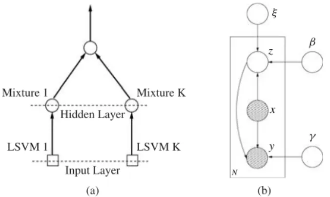
In this section, we present our MLSVM model. Without loss of generality, we illustrate our model with a two-layer mixture model as shown in Fig. 1(a). Generalization to hier-archical mixtures is straightforward and will be discussed in Section III-E. The model in Fig. 1(a) consists of two parts. The hidden layer is composed of the gating network that produces a soft partition of the input space by generating a data-dependent
ξ z y β γ x N (b) (a) Hidden Layer Input Layer LSVM 1 LSVM K Mixture 1 Mixture K
Fig. 1. MLSVM model. (a) Model topology. (b) Graphical model representation.
weight distribution. Each node in the hidden layer is connected to a LSVM classifier in the input layer, which is responsible for the classification of data points residing in the corresponding partition.
The proposed mixture model captures the posterior proba-bilistic distributions of the labels Y given input data X by
P(Y|X, ) = i P(yi|xi, ) = i zi ξziP(zi|xi, β)P(yi|zi,xi, γ ) (6) where i indexes correspond to the data samples and =
{ξ, β, γ}are the parameters of the underlying model. In the expression above, we have assumed that the training instances/labels are independent and identically distributed (i.i.d.) and zi is the hidden variable introduced for the i th
instance that takes values in {1, . . . ,k}, where k is the total number of mixtures. The weight of the i th instance is deter-mined by bothξzi and P(zi|xi, β). The data-independent term
ξzi specifies the prior probability of the mixture component indexed by zi, whereas the data-dependent term P(zi|xi, β)
specifies the probability model for the gating function and is related to the importance of the i th instance with respect to the zith mixture component. P(yi|zi,xi, γ ) is governed
by the classification process for the zith component and
specifies the posterior probability of the i th instance output by the corresponding LSVM model. The parameters for the gating functions are given by β and γ, respectively. We elaborate further on their specific parametric forms later in this paper.
Our MLSVM model can also be visualized by a graphical model as shown in Fig. 1(b). In this figure, x and y are the target variables over which the probability model is defined, and z is the hidden variable. The box containing x , y, and z indicates i.i.d. copies of variables, where N is the number of copies. The arrows indicate dependences between the vari-ables, where the variable pointed by an arrow is conditionally dependent on the variable where the arrow originates from.
The mixture model is generated from a multinomial dis-tribution with parameter ξ = {ξ1, . . . , ξk} for k-mixture. The posterior probability P(z|x, β) is specified by the
following equation: P(z= j|x, β)= exp −τx−vj2 jexp −τx−vj2 . (7)
The parameter β = {v1, . . . ,vk} specifies the centroid of each component. The probability for each centroid is determined by the Euclidean distance between the instance and the centroid location. The closer the distance, the larger the probability. The assignment of instances to the components is probabilistic in nature, where τ is a scale parameter that controls the softness of the assignment. The smaller the value of τ, the “softer” the assignment. In the extreme case when
τ = 0, the gating function produces equal weights for all components. On the other hand, whenτ approaches infinity, the gating function returns 1 for the closest component and 0 for the others. The probability P(y|z,x, γ )is governed by the classifier model with parameterγ conditional on x and z, whereγ = {w1, . . . ,wk}and wj is the parameter for the j th
LSVM. We can clearly see the correspondence between the graphical model and the probability distribution in (6).
It is worth noting that the proposed MLSVM model bears some resemblance with the classical mixture-of-expert model proposed by Jacobs and Jordan [4]. Nonetheless, there are two main differences. Firstly, our model is a mixture of weighted experts and more general in nature. This is because the mixture-of-experts model can be treated as a special case of ours with the mixing coefficientsξj set to 1/k. The explicit
use of mixing coefficients enables us to perform implicit model selection via enforcing a sparseness prior over ξ as we will discuss in the following section. For the mixture-of-expert model, however, there is no way to control the model structure by enforcing constraints on the parameters, and we have to resort to heuristics for explicit model selection [9], [10]. Secondly, we have used a nonlinear RBF gating function in (7), whereas the mixture-of-expert model adopted a linear function for the gating network. Hence our model is more flexible in generating the partitions over the data space than the of-expert model. Note that an alternative mixture-of-expert model was proposed in [11], which also makes use of the RBF gating function by modeling the joint distributions of the data and labels in a generative manner. Hence, it is not directly comparable with discriminative models for classification such as the one proposed in this paper.
Following the maximum likelihood estimation (MLE) prin-ciple, the parameters of our classification model can be esti-mated by maximizing the log-likelihood function
L() = i log P(yi|xi, )+ j (wj) = i log j ξjP(zi = j|xi,vj)P(yi|xi,wj) + j (wj) (8)
where(wj)=log(P(wj))specifies the log-prior term over
the SVM parameters for purpose of regularization and P(zi =
In order to incorporate LSVMs into the above MLE frame-work, we have to reformulate it from a probabilistic viewpoint. To this end, we view the constrained quadratic optimization problem in (1) as that corresponding to the negative log-likelihood of the energy function whose first term on the right-hand side is related to the prior (w) and the second term corresponds to the conditional probability P(y|x,w) related to classification error. These are given by
(w)= −ζ||w||2 (9)
P(yi|xi,w)=e−(w;xi,yi). (10)
Here we have omitted the normalization factor for the conditional probability P(yi|xi,w), which leads to an
ap-proximation of the probability measure. This is mainly for the convenience of numerical optimization, which enables us to use the existing fast LSVM solvers [8] during parameter estimation. This simplification is particularly valid in the large-margin case where the probability of misclassification is usually very small. More importantly, from an optimization point of view, we can still apply the EM algorithm to optimize the likelihood function in (8), which is guaranteed to increase in each EM iteration regardless of whether P(yi|xi,wj)is a
proper probability measure over yi as we will discuss in the
next section. The posterior probability is unity, i.e., zero loss, for instance xi if and only if it has a margin greater or equal
to unity, i.e., yi(wTxi+b)≥1.
B. The EM Algorithm
Now, we turn our attention to the use of the EM algorithm for solving the MLSVM model presented in the previous section. The E-step updates the posterior probabilities of assigning each instance to the component classifiers. Let
(t) = {θ(t) j }j=1,...,k = {ξ (t) j ,v (t) j ,w (t) j |j = 1, . . . ,k} be the
parameters at the current iteration, the probability of assigning the i th instance to the j th classifier at iteration t is
qi(,tj)= ξ (t) j P zi = j|xi,v(jt) P yi|xi,w(jt) jξ( t) j P zi = j|xi,v(jt) P yi|xi,w(jt) (11)
where P(zi = j|xi,v(jt)) and P(yi|xi,w(jt)) are posterior
probabilities associated with the gating networks and local experts at iteration t given by (7) and (10), respectively.
The M-step involves simultaneously updating the parame-ters for the gating functions and SVM classifiers. This involves solving two independent optimization problems. For the gating functions, the values of the mixing coefficientsξj at iteration
t+1 can be obtained in closed form
ξ(t+1) j = iq( t) i,j N . (12)
Estimation of the centroid parameters for the gating func-tions is equivalent to unconstrained optimization. Specifically, for the j th mixture component, the centroid vj is updated by
solving the following optimization problem: v(jt) =arg min vj f(vj) =arg min vj ⎧ ⎨ ⎩− i,j qi(,tj)log P(zi = j|xi,vj) ⎫ ⎬ ⎭ (13) where P(zi = j|xi,vj)is defined in (7). The above problem
is very similar to parameter estimation for logistic regression and can be tackled by widely available numerical routines for unconstrained optimization [12]. Here, we adopt a lim-ited memory BFGS (L-BFGS) method sulim-ited for large-scale optimization [13] to minimize the cost function in (13). The L-BFGS method requires only the gradient information of the cost function for the past few iterations, which can be calculated by ∇vj f(vj)=2β i qi(,tj)−P zi = j|xi,v(jt) v( t) j −xi . (14) Furthermore, it is worth noting that we do not have to solve the optimization problem associated with the parameters v(jt) in (12) for each iteration. We can initialize the L-BFGS method for each iteration with the values v(jt−1), since the parameters change slowly across iterations. This can greatly reduce the time for parameter estimation and speed up the training process.
Parameter estimation for the LSVMs reduces to updating the classifiers for reweighted samples where the weights are specified by the posterior probabilities computed in the E-step. Specifically, for the j th linear classifier, we solve the following classification problem: max iq( t) i,jlog P yi|xi, θ(jt) +log P θ(t) j =max −iq( t) i,j w(jt);xi,yi −ζw(jt) 2 . (15) This is exactly the same problem as the training of LSVMs in (1) with sample weights given by qi(,tj) and C = 1/2ζ. Again, for every iteration we can train the weighted LSVMs in incremental manner via updating the results from the previous iteration. Since we have used a dual coordinate descent method for solving LSVMs, we have retained the dual variables as well as status variables for each LSVM in each iteration for their use by the corresponding LSVM for the next iteration. This can be done via trivial adaptation of the original training algorithm and can greatly reduce the time spent for LSVM training to a great extent.
Each EM iteration increases the log-likelihood given by (8). This argument can be easily established by making use of the auxiliary function parameterized with respect toθ(t) given by Q (t);(t−1)= i,j qi(,tj)logξjP zi=j|xi,v(jt) P yi|xi,w(jt) − i,j qi(,tj−1)log qi(,tj−1)+ j w(jt−1) (16)
which is the lower bound ofL((t))since
L(t)−Q(t);(t−1)=q(t−1) i,j log
qi(,tj−1)
qi(,tj) . (17) The gap is nonnegative and varnishes if and only if θ(t)=
θ(t−1). Hence the log-likelihood increases with the following
relation: g (t) ≥ Q(t);(t−1) ≥ Q (t−1), (t−1)= g (t−1).
The second inequality is true because of the maximization step. Therefore, by repeating the EM steps in an interleaved manner, we can obtain a convergent solution of the original MLE problem.
C. Model Selection
Model selection is a challenging problem for learning mix-ture models, which involves estimating the number of mixmix-ture components. The dominant approach for doing so relies on optimizing certain criteria via a search over a range of number of components k∈ [kmin,kmax]such that
ˆ
k=arg min
k {−log P(X|k)+R(k)}
where we have writtenk so as to denote the estimate for the candidate value when the number of components is set to
k andR(k)is a function that penalizes large values of k. The
first term on the right-hand side is related to MLE, whereas the second term is related to model complexity. Examples of criteria for complexity that have been used for mixtures include Bayesian inference criterion, minimum description length, MML, and so on [2].
One major disadvantage of the above deterministic ap-proach is that parameter estimation and model evaluation are performed independently, and one may have to do an exhaustive search over a large interval of k and run separate parameter estimation process for each of them to obtain an optimal estimate. To sidestep this difficulty, we adopt an alternative approach that couples parameter estimation and model selection in a unified framework. We start with an overcomplete model with a large number of components and implicitly select the components in a top-down manner. This is achieved by enforcing priors on the mixing coefficients
ξj, where the components with vanishing coefficients are
annihilated automatically in the training process. Following [14], we adopt the Dirichlet-type prior forξj which is given by
P(ξ)∞exp ⎛ ⎝−νk j=1 logξj ⎞ ⎠ (18)
where ν is a tradeoff parameter for the balance between the data and the complexity terms. Incorporating it into the log-likelihood function in (8) leads to the following overall log-likelihood:
()=L()+log P(ξ)=L()−ν
j
logξj. (19)
Input: Labelled sample {xi,yi| = 1, . . . ,N} andkmax Output: ParameterΘ{ξj, vj,wj|j =1, . . . ,k}
• InitialiseΘfork =kmax.
• E-step:calculate qi,j via Equation 11. • M-step:
– updateξj’svia Equation 20.
– update vj via Equation 13 for all j such thatξj=0. – update classifierswj’s for all j such thatξj=0 by
re-traininglinear SVM in Equation 15. • Repeat the above two stepsuntil convergence.
Fig. 2. Algorithm for our MLSVMs.
The advantages of using the above Dirichlet-type prior are twofold. Firstly, it enforces sparseness over ξ and hence penalizes complex models with many components. Secondly, it is the conjugate prior of multinomial random variables. Therefore,ξ can be computed in the closed form
ξj = max 0,iqi(,tj)−ν jmax 0,iq( t) i,j −ν . (20)
It is worth noting that here the only difference from the EM algorithm developed in the previous section is in the estimation ofξj ∈ξ.
D. Algorithm and Implementation
We now present the step sequence of the MLSVM algorithm in Fig. 2. We start with a relatively large kmax and apply
component elimination in the parameter estimation process. K-means clustering is used to initialize EM. Specifically, we divide all training instances into k clusters and apply a LSVM to instances from each cluster. The cluster centroids are initial values of v’s for the gating function in (7) and initial SVM parameters yielded by the LSVM applied to each cluster. In the case that any cluster contains only instances from a single class, one can initialize the corresponding SVM weight to ed+1
for clusters containing only positive instances and −ed+1 for
those clusters comprised of negative instances, where ed+1 is
a d+1-dimensional vector whose entry indexed d+1 is unity and 0 for all others. In each M step, the SVM classifiers are updated from the weights from the previous iteration. This is much faster than training from random initialization since, in practice, the classifiers do not change abruptly between subsequent iterations.
There are two free parameters to be tuned in our model: the regularization parameter C for the LSVM, and the reg-ularization parameter ν for the prior term over ξ. These two parameters control the complexity of the LSVM as well as the overall mixture model and can be chosen via cross validation.
In the testing stage, a novel testing data point is classified by the weighted average over the classifier mixture as given
by the discriminant function ξj=0 ξjP(zi = j|x,vj) emax 0,1−wT jx −emax 0,1+wT jx . (21) Prediction is made by the sign of the discriminant function. Despite the complicated form of the function, it is straightfor-ward to see that it has a low computational complexity, which is linear in the number of mixture components with nonzero coefficients.
E. Extension to a Hierarchical Mixture
Similar to the extension from mixture of experts to the hierarchical mixture model (HME) [15], it is natural to extend MLSVM to the HME. For a three-layer network with two hidden layers of gating functions, we have the following probability model: P(Y|X, )= n i j ξijP(rn= j|xn,ui) ×P(zn=i|xn,vi,j)P(yn|xn,wi,j) (22) where rn and zn denote the hidden variables for the selection
of the gating units at the first and second hidden layers. In the equation above, ξi and j are the data-independent weights
for the i th gating unit in the first layer and the j th gating unit in the second layer, which is connected to the i th unit in the first layer. The probabilities P(rn = j|xn,ui) and
P(zn = i|xn,vi,j) specify the data-dependent posteriors for
the corresponding gating units.
Note that, for the hierarchical mixture above, we can still apply the EM algorithm to estimate the model parameters with slight modifications in the estimation of mixing coefficients. Model selection can also be achieved by imposing the same prior on the mixing coefficients, where a component is anni-hilated if its correspondingξi orj are negligible. In practice,
the single-layer mixture model, which acts like a RBF kernel SVM, is capable of handling most classification problems arising in practical applications. On the other hand, the hier-archical model, despite its elegant theoretical underpinnings, is prone to overfitting because it is difficult to regularize the model. Hence, in this paper, we focus on the use of a single-layer MLSVM.
IV. DISCUSSION
The motivation of the work presented in this paper is quite different from that elsewhere in the literature. Competing approaches [16]–[18] employ a divide-and-conquer strategy similar in spirit to the mixture-of-expert framework [4] in the partitioning of the input space into disjointed regions. Once the space has been partitioned, a local nonlinear SVM classifier is trained on samples falling in each region. Again, this may greatly reduce the training time but does not create the efficiency for prediction due to the use of nonlinear SVMs as local experts. A straightforward remedy might be to replace the nonlinear SVMs with their linear counterparts.
Note that, in general, there is no guarantee that the training data in each region are linearly separable. Moreover, as mentioned in Section III-C, model selection is a hard problem for the HME. Previous methods for model selection applied to the mixture of experts [4] and its hierarchical extension [15] have been addressed by several authors [9], [10], [19], [20]. However, all of these approaches are focused on the use of heuristic bottom-up procedures that start with a small network and grow it adaptively for learning the topology of the network. This process can hardly be automated and, thus, in practice, a fixed number of components is usually used in mixture of expert learning. The work presented in this paper is most similar in nature to the LSVM mixture model proposed in [21], which is directly based on the mixture-of-experts model [4] for LSVMs. To the best of our knowledge, the problem of locally linear learning for fast prediction with automatic model selection has not yet been investigated.
Along a different line of research, approximation-based methods have been widely used for nonlinear SVMs to ac-celerate the process of training them for large-scale data. Such methods are based on approximating the kernel matrix with the outer product of linear vectors spanned by a set of basis functions. The bases can be obtained by using low-rank decomposition methods like incomplete Cholesky factorization [22], [23] or the Nystrom approximation [24]. Alternatively, they can also be chosen randomly following certain princi-ples [25], [26]. Despite effective in speeding up the training process, kernel approximation methods come at an expense for the efficiency in testing. This is due to the fact that the linear features are obtained on top of the kernel matrix. Hence, the full kernel matrix needs to be computed in the testing phase, which breaks the sparsity of SVs and further slows down the prediction process.
Another natural choice for combining linear classifiers for nonlinear classification is ensemble methods such as bagging [27], boosting [28], and random forests [29]. These methods are quite effective in learning combinations of weak classifiers for classification of data with complicated distributions, yet they do not enforce sparseness on the hypothesis space. Therefore, when linear classifiers are used as the base learner, ensemble methods tend to use a greater number of them for difficult cases compared to our approach and thus are likely to increase the time spent on prediction. Moreover, ensemble methods are best combined with unstable base learners, such as decision trees, to fully exploit different random natures of the weak learners for combination. For stable classifier models like SVMs and artificial neural networks, the training process is quite robust to data perturbation. Thus, the classifiers ob-tained at different stages are likely to be highly correlated. This would not only increase the number of iterations required for convergence but, more importantly, would negatively affect the performance of the combination scheme with such classifiers used as weak learners.
V. EXPERIMENTS
In this section, we demonstrate the performance of the proposed algorithm on both synthetic and real-world data.
2 1.5 1 0.5 0 −0.5 −1 −1.5 −2 −1.5 −1 −0.5 0 0.5 1 1.5 2 −2 −1.5 −1 −0.5 0 0.5 1 1.5 2 −2 −1.5 −1 −0.5 0 0.5 1 1.5 2 −2 −1.5 −1 −0.5 0 0.5 1 1.5 2 −2 −1.5 −1 −0.5 0 0.5 1 1.5 2 −2 −1.5 −1 −0.5 0 0.5 1 1.5 2 −2 −1.5 −1 −0.5 0 0.5 1 1.5 2 −2 35 30 25 20 Err Rate (%) 15 10 5 0 0 −20 −60 −40 −100 −80 Lo g -likelihood−120 −160 −140 −200 −180 −220 2 1.5 1 0.5 0 −0.5 −1 −1.5 −2 2 1.5 1 0.5 0 −0.5 −1 −1.5 −2 2 1.5 1 0.5 0 −0.5 −1 −1.5 −2 2 1.5 1 0.5 0 −0.5 −1 −1.5 −2 2 1.5 1 0.5 0 −0.5 −1 −1.5 −2 2 1.5 1 0.5 0 −0.5 −1 −1.5 −2 0 10 20 30 40 Iterations 50 60 70 80 90 100 0 2 4 6 8 Iterations10 12 14 16 18 20
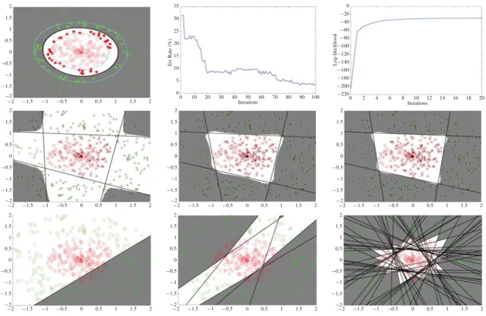
Fig. 3. MLSVM versus boosting on synthetic two-class data. Top row, from left to right: decision boundary of nonlinear SVM, test error of Bst-SVMs, and log-likelihood of our algorithm as a function of iteration number. Middle row: results of our algorithm at the initial, fifth, and final iterations. Bottom row: results for the Bst-SVMs at the first, tenth and final iterations.
Two real-world applications are considered: namely optical character recognition (OCR) and hyperspectral image clas-sification. We compare our MLSVM algorithm with LSVM, nonlinear SVMs with the RBF kernel, and boosted LSVMs. The boosting algorithm used here is AdaBoost [28]. Unless otherwise stated, in our framework we have set the initial number of LSVMs to 10. The final number of linear models, however, might be less than 10 due to the implicit model selection ability of the proposed MLSVM algorithm in Fig. 2. We empirically set the parameter τ in (7) to unity. Note that
τ may also be treated as an independent parameter whose value can be chosen via cross validation. In practice, we have experimented with different settings of τ and found that its value does not have much impact on the classification perfor-mance. We have chosen the other parameters for MLSVM and the alternatives via fivefold cross validation. LibSVM [30] and LibLinear [8] were used for training kernel and the LSVMs, respectively. For boosted LSVMs, we have used the optimal regularization parameter obtained via cross validation and fixed the number of boosting iterations to 100.
Fig. 3 shows the toy binary dataset used in our synthetic data experiment, where 200 positive instances are shown in red circles, which occupy the circular region in the middle, surrounded by 200 negative instances in green circles. The instances are chosen by subsampling a large sample of in-stances generated by uniform distribution within the square region. Clearly, the instances from these two classes are not linearly separable. The top row, from left to right, shows the decision boundary recovered by kernel SVMs, test errors of
boosted SVMs (Bst-SVM) over sample iterations, and the log-likelihood values of MLSVM as given by (8). We have fixed the number of components to 4 for the MLSVM. For the nonlinear SVM, the decision boundary is plotted in black. The decision boundaries with margin values of 1 corresponding to the two classes. The SVs are shown in solid circles. Even for this simple example, the SVM with RBF kernel yielded 71 support vectors, which is not particularly efficient for large-scale prediction tasks. For the Bst-SVMs, we can see that the training error reduces slowly and becomes stable only after a large number of iterations. This has confirmed our previous assertion that boosting requires many iterations to converge. For MLSVM, on the other hand, we can see that the log-likelihood value increases with every iteration and requires only a few iterations for convergence.
This is further justified by the plots in Fig. 3. In the middle row of the figure, from left to right, we show the results of MLSVM at the initial, fifth, and final iterations. In each plot, the digit in each circle indicates the index of the mixture com-ponent for the training instances. The shaded regions indicate negative classes, whereas white indicates positive classes. It can be seen that the classification model learned by the fifth iteration is already in good accordance to that yielded by the final iteration. This is in contrast with the boosted LSVM model, which is constantly evolving. This can be seen from the results recovered by the boosting model at the first, tenth, and final iterations as shown in the bottom row of the figure. Since boosting is a greedy strategy for classifier combination, it uses a much larger number of weak classifiers, most of which aim
5 0 25 −25 20 −20 15 −15 10 −10 −5 −25 −10 −5 0 5 10 15 20 25 5 0 25 −25 20 −20 15 −15 10 −10 −5 −25−20−15−10 −5 0 5 10 15 20 25 5 0 25 −25 20 −20 15 −15 10 −10 −5 −25−20 −15 −10 −5 0 5 10 15 20 25 5 0 25 −25 20 −20 15 −15 10 −10 −5 −25−20−15−10 −5 0 5 10 15 20 25 5 0 25 −25 20 −20 15 −15 10 −10 −5 −25−20 −15−10 −5 0 5 10 15 20 25 −260 −280 −320 −200 −300 −220 −240 80 20 30 40 Iterations 50 60 70 10 0 Lo g -likelihood −20 −15
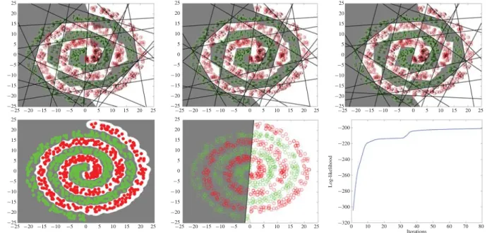
Fig. 4. MLSVM versus SVM on the synthetic spiral dataset. Top row: results for our MLSVM at the initial, tenth, and final iterations. Bottom row, from left to right: decision boundaries of nonlinear and LSVMs, and log-likelihood of MLSVM as a function of iteration number.
at correcting errors incurred in previous iterations. This has the counterproductive effect of canceling the effects of one another. More importantly, unlike the MLSVM, each boosting iteration introduces a new classifier into the ensemble model. Hence, boosting has to combine a lot more linear classifiers than the proposed algorithm to yield comparable performance. Even for this simple dataset, boosting employs approximately 100 LSVMs to achieve a comparable performance to that of MLSVM, which only used 4 classifiers.
To further demonstrate the power of MLSVM for the recovery of complex decision boundaries, we performed clas-sification on a second synthetic dataset comprised by two spirals intertwined with each other, as shown in Fig. 4. Each spiral has five turns and consists of 500 instances. These are generated by subsampling a larger sample of instances uniformly distributed around the spiral curve given by the polar function r =1.3θ(−1.3θ)whose independent variable is θ ∈ [0.5 π,5.5 π]. This is a hard classification problem because of the high nonlinearity of the dataset. We have trained our MLSVM classifier with 20 linear classifiers. The top row, from left to right, shows the results obtained by MLSVM in the initial, tenth, and final iterations. In each plot, the digit in each circle indicates the index of the mixture component for the training instances. The shaded regions indicate negative classes, whereas white indicates positive classes. It can be seen that MLSVM can model rather complicated decision boundaries through mixing the linear classifiers.
Furthermore, the decision boundary of MLSVM is refined over iterations, from initially correctly classifying 95.7% of the data to 99.7% in the final iteration. This is further justified by the increased log-likelihood over iterations as shown by the rightmost plot in the bottom row of the figure. The first two plots in the bottom row show the decision boundaries produced by RBF kernel-based nonlinear and LSVMs, respectively. The linear decision boundary returned by the LSVM achieves only a random classification rate of 50%. This also invalidates the
use of the boosted SVM model, as boosting requires at least better than random classification performance at each iteration to proceed. The nonlinear SVM achieves 100% accuracy with a smoother decision boundary than that of MLSVM. However, this is at the cost of generating over 750 support vectors in the training process so as to approximate such complicated decision boundary. This accounts for over three-quarters of the training set and about 20 times the complexity of our MLSVM, which uses only 20 linear classifiers.1 For the 2-D spiral dataset, it takes 70 ms for the nonlinear SVM prediction and 3.5 ms for our MLSVM. The experiments were effected on an Intel 3.0-GHz Core 2 Duo desktop with 4 GB RAM. Training MLSVM is more expensive than SVM, which takes 5 s, as compared to only 0.5 s for the LSVM with a fully optimized LibSVM routine. However, training can be done offline for most pattern classification problems, whereas prediction must be performed online. Hence online prediction efficiency is often more important especially for large-scale problems, which is the main focus of our MLSVM method.
Now we turn our attention to real-world data. We first demonstrate the performance of our algorithm for OCR on the MNIST database [31]. The database contains 60 000 training images and 10 000 testing images of handwritten digits from 0 to 9. We have divided them into two classes, one for the odd numbers and another one for the even digits. The resolution of each image is 28×28, which leads to a 784-dimensional feature vector by concatenating the pixel values columnwise. We have trained the algorithms under comparison over subsets of different sizes drawn randomly from the training set and applied them to the testing set. We have repeated this procedure 10 times and recovered quantitative results regarding classification performance.
1Note that the complexity of MLSVM scales with twice the number of linear classifiers, including gate function and classifier evaluations.
TABLE I
OCR PERFORMANCE. COMPARISON OFLSVM, NONLINEARSVM, BST-SVMS,AND THEPROPOSEDMLSVM
Training Size LSVM (%) SVM (%) Bst-SVM (%) MLSVM (%) 100 80.62±2.33 84.70±1.21 80.62±2.33 82.82±1.97 500 82.71±0.80 91.71±0.96 82.71±0.80 90.12±1.43 1000 84.71±0.53 94.59±0.21 83.67±0.24 92.82±0.26 5000 88.47±0.28 97.30±0.16 87.40±0.24 93.91±0.33 10 000 89.60±0.13 98.01±0.09 88.98±0.21 94.89±0.23 All 90.28 98.49 89.72 95.20 TABLE II
OCR COMPLEXITY. NUMBER OFSUPPORTVECTORSUSED BY THENONLINEARSVMAND
NUMBER OFCLASSIFIERSEMPLOYED BYBOOSTING(BST-SVM),AND THEPROPOSEDMLSVM
Training size SVM Bst-SVM MLSVM
Mean Min Max Mean Min Max Mean Min Max
100 79.2 69 86 1 1 1 5.2 2 8 500 263.2 236 288 1 1 1 5 2 7 1000 428.8 414 446 100 100 100 8.8 8 10 5000 1178.4 1157 1202 100 100 100 8.6 8 10 10 000 1817.0 1800 1833 61.8 24 100 8.6 7 10 All 3564 100 10
Table I shows the classification rates on the test set in terms of accuracy for MLSVM and the alternatives. It can be seen clearly that the nonlinear SVM outperforms the other methods. It delivers the highest classification accuracy followed by our MLSVM model. The MLSVM is comparable in performance with nonlinear SVM on small sample sizes and is better than LSVMs regardless of the size of training dataset. The performance of boosted LSVMs is, however, unsatisfactory for the OCR task. For small training sample sizes, it achieves only the same performance as the LSVM. This may be due to the fact that the randomly selected subset of the training data is most likely linearly separable, which leads to the early stopping of the boosting procedure in the first iterations. This is confirmed by the number of iterations used for boosting reported in Table II. For larger training sizes, the performance of boosting slightly decreases with increasing number of iterations, as reported in the last four rows of Table I. This suggests that Bst-SVMs are not the model of choice for bridging between the complexity of nonlinear SVMs and the performance of linear classifiers. On the contrary, boosting appears to have a higher complexity for increasing number of iterations and lower performance as compared to LSVMs. Our MLSVM model, on the other hand, clearly outperforms LSVMs for OCR and is much more efficient than the nonlinear SVM. It is worth noting that, although the training data are likely to be linearly separable for small sample sizes, their distributions are inherently nonlinear. Hence, nonlinear SVMs still achieve higher classification accuracy than their linear counterparts. Our MLSVM can implicitly exploit the nonlinear nature of the dataset and deliver better performance than the LSVM for small sample sizes.
We also compare the complexity of the methods under study. Table II shows the complexity for Bst-SVMs and MLSVM as measured in terms of number of linear classifiers used. For the nonlinear SVM, we list the number of SVs as a measure of complexity. Notice that, for different training data,
SVMs may produce different number of support vectors. Our proposed MLSVM method may also select different number of linear classifiers via the training algorithm in Fig. 2 with implicit model selection. For each training data size, we have listed the average, minimum, and maximum number of linear classifiers/SVs used over all the training rounds. From the table, note that that the complexity of the nonlinear SVM grows with increasing training data sizes. This is because the number of SVs obtained in the training process is proportional to the size of training set. The proposed MLSVM model, on the other hand, is not affected by the size of the training dataset. As can be seen from the table, it is much more efficient than the nonlinear SVM. Further, it is orders of magnitude faster for large training data sizes. For instance, it takes the nonlinear SVM 27, 46, and 195 s, on average, for the prediction of 10 000 testing instances given training sets of sizes 5000, 10 000, and all available data. On the other hand, the LSVM takes, on average, only 10 ms and MLSVM 0.7 s for the same prediction task regardless of the sizes of the training dataset. Nevertheless, the MLSVM takes an hour for training using the full training dataset, as compared to 1 and 2 min for the nonlinear and LSVMs, respectively.2Again, as we argued before, this is not essential, as training can be performed offline. The behavior of Bst-SVMs is quite unex-pected. For small training sizes, the randomly drawn training dataset is likely to be linearly separable, so boosting stops at the first iteration with zero training error. For larger training sets, it requires a large number of iterations to converge. Since each boosting iteration introduces a new classifier in the ensemble model, this greatly increases the complexity of the model.
2We found the timing results for training quite unusual, with the nonlinear SVM outperforming LSVMs in training speed. This also greatly affects the speed of our MLSVM method, as it calls LSVM solvers frequently for training. This is counterintuitive, since LibLinear, the solver we used for LSVM training, should scale linearly with training sample sizes [8].
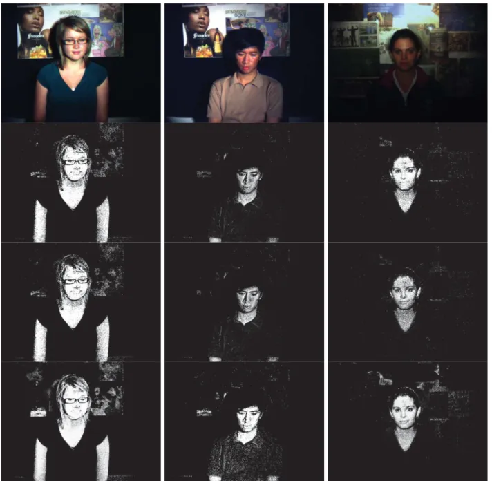
Fig. 5. Example skin classification results. Top row: pseudo-color images for sample human subjects. Second, third, and fourth rows: classification results delivered by our algorithm, the nonlinear SVM and LSVM, respectively.
We repeated the experiments above on the Forest Cover-type dataset. This is a dataset presented in [32] derived from data originally obtained from U.S. Geological Survey data by the Colorado State University.3 The dataset contains 581 012 instances from seven cover types. Each instance has 54 feature attributes capturing cartographic information. The purpose is to predict various cover types from the cartographic variables. We converted this to a binary classification prob-lem by predicting whether each instance belongs to cover type 2, which is the largest cover type, containing 283 301 instances, i.e., approximately half the dataset. As for the OCR experiments, we compare the performances of our MLSVM algorithm and the alternatives using different training dataset sizes. Training instances were randomly drawn from
3The data set can be found at http://kdd.ics.uci.edu/databases/covertype/.
the full dataset and the rest were used for prediction. The procedure was repeated 10 times. The average accuracy rates along with standard deviations are shown in Table III. We show the time complexities in Table IV.
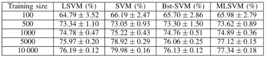
The trend on the forest cover prediction data is similar to that for the OCR. The nonlinear SVM achieves the best performance, followed by the MLSVM. Both of them perform better than the LSVM. On the other hand, the nonlinear SVM has the highest complexity for prediction. It is much more costly than the MLSVM and LSVM. Moreover, the MLSVM achieves the optimal tradeoff between prediction performance and complexity. Given sufficient training data, the cost of MLSVM is almost independent of the training data size. This is in contrast with the nonlinear SVM, whose complexity scales with the number of training data used. This is further justified by the average testing speed. The nonlinear SVM
TABLE III
PERFORMANCECOMPARISON OF THELSVM, NONLINEARSVM, BST-SVMS,
AND THEPROPOSEDMLSVM ALGORITHM ON THEFORESTCOVER-TYPEDATASET
Training size LSVM (%) SVM (%) Bst-SVM (%) MLSVM (%) 100 64.79±3.52 66.19±2.47 65.70±2.86 65.98±2.79 500 73.34±1.10 73.05±0.93 73.30±1.50 73.62±0.89 1000 74.78±0.47 75.22±0.43 74.76±0.51 74.89±0.36 5000 75.97±0.20 78.92±0.29 76.06±0.25 77.12±0.15 10 000 76.19±0.12 79.98±0.16 76.13±0.12 77.34±0.18 TABLE IV
COMPLEXITYCOMPARISON FOR THEFORESTCOVER-TYPEDATA. NUMBER OFSVSUSED BY THENONLINEARSVM
ANDNUMBER OFCLASSIFIERSEMPLOYED BY THEBOOSTINGALGORITHM(BST-SVM)ANDOURPROPOSEDMLSVM METHOD
Training size SVM Bst-SVM MLSVM
Mean Min Max Mean Min Max Mean Min Max
100 74.2 68 80 61.9 13 100 3.4 1 10
500 323.9 286 356 33.9 10 62 1.4 1 3
1000 604.9 571 635 61.0 20 100 2.1 1 6
5000 2643.4 2568 2743 60.5 29 100 4.5 1 10
10 000 5028.6 4934 5121 53.3 19 100 4.2 1 9
takes 40, 167, and 281 s for prediction given training set sizes of 1000, 5000, and 10 000, respectively. Our MLSVM method takes 2 s and the LSVM takes 50 ms for prediction regardless of the sizes of the training dataset. Boosted LSVMs are inferior to the other methods being studied and do not achieve any improvement over LSVM.
We now turn our attention to the application of our MLSVM algorithm to pixel-level skin classification in hyperspectral images. Here, we aim at exploiting the information-rich rep-resentation of the scene in hyperspectral imaging. To this end, we have used a set of 696×520 images of human subjects captured in-house against a cluttered background making use of a hyperspectral camera sensor. Each pixel in the image has 33 spectral channels covering the narrow-band spectral reflectance in the visible range from 400 to 720 nm in steps of 10 nm.
Example pseudocolor images of some of the subjects under study are shown in the top row of Fig. 5. For purposes of training, we have selected patches enclosing the skin areas from a few images. The spectral feature vectors were then obtained using the photometric invariant preprocessing method in [33]. Since Bst-SVMs do not produce satisfactory results in terms of either classification accuracy or efficiency of predic-tion, we have focused our comparison on the remaining three algorithms. Some example skin classification results are shown in the two bottom rows of Fig. 5. These correspond, from top to bottom, to the results yielded by the MLSVM, the nonlinear SVM with RBF kernel, and the LSVM. We can see that the skin maps recovered by the MLSVM are quite similar to those yielded by the nonlinear SVM, whereas the skin maps com-puted using the LSVM are less accurate than those correspond-ing to the other two methods. Furthermore, from the figure we can see that the skin maps returned by the LSVM contain more false positives than those yielded by the MLSVM. This is particularly evident on the small regions in the background wallpaper, which have been falsely classified as skin.
In Table V, we show a more quantitative analysis of the performance for the alternatives under study. This includes
TABLE V
AVERAGECROSS-VALIDATIONERROR ANDTESTINGTIME FORSKINCLASSIFICATION
MLSVM SVM LSVM
Accuracy 95.20±0.30 95.45±0.22 91.34±0.15 Time (s) 6.55±0.25 76.25±1.30 1.65±0.05
the average testing accuracy as well as the average testing time in seconds per image. The average testing accuracy is measured by splitting the training data into two sets, one for training and the other one for testing. This is done by evenly splitting the dataset and averaging the results over five different random partitions. From the table, we again notice that the MLSVM is much more efficient while achieving a performance comparable to that yielded by the nonlinear SVM. The LSVM, on the other hand, is quite efficient for testing but has a lower accuracy rate as compared to the nonlinear SVM and our MLSVM approach.
VI. CONCLUSION
In this paper, we have proposed the MLSVM. This is a novel method to combine linear classifiers for the classification of nonlinear data. We have addressed the problem by casting it into a probabilistic setting so as to implicitly perform model selection. This is done by using the EM algorithm on a generative model, which permits the use of priors on the mixing coefficients. Our MLSVM method provides a means to efficient nonlinear classification by presenting a top-down parameter estimation process. The method is quite general in nature and is particularly well suited for large-scale prediction tasks. We have done experiments on synthetic and real-world data and provided comparison to boosting, linear, and nonlinear SVMs.
There are a number of possible directions for future re-search. One potential application of the proposed framework is feature combination, where each example in the dataset is represented by multiple feature vectors extracted from differ-ent sources. The standard approach to solving this problem
with SVM is multiple kernel learning (MKL) [34], [35], where individual kernel matrices computed from different features are linearly combined. MKL is then formulated as a joint optimization problem over the kernel combination weights and the SVM classifier. Unfortunately, testing can be computa-tionally expensive for large datasets with many input feature types [35]. The method proposed here can learn a MLSVMs. This can be done separately for the individual features so as to combine the output scores. Another option is to combine feature types directly, making use of the joint feature vectors. The mixture model can capture the nonlinear information in each individual feature while still maintaining efficiency in prediction. Another possible extension is the use of error-generalization bounds for parameter selection [36], [37]. This is especially effective for small sample size problems and provides a more accurate estimate of the prediction error than that given by cross validation.
REFERENCES
[1] B. Schölkopf and A. Smola, Learning with Kernels: Support Vector Machines, Regularization, Optimization, and Beyond. Cambridge, MA: MIT Press, 2001.
[2] J. Rissanen, Stochastic Complexity in Statistical Inquiry. Singapore: World Scientific, 1989.
[3] A. P. Dempster, N. M. Laird, and D. B. Rubin, “Maximum-likelihood from incomplete data via the EM algorithm,” J. Royal Statist. Soc. B, vol. 39, no. 1, pp. 1–38, 1977.
[4] R. A. Jacobs, M. I. Jordan, S. J. Nowlan, and G. E. Hinton, “Adaptive mixtures of local experts,” Neural Comput., vol. 3, no. 1, pp. 79–87, 1991.
[5] C.-W. Hsu and C.-J. Lin, “A comparison of methods for multiclass support vector machines,” IEEE Trans. Neural Netw., vol. 13, no. 2, pp. 415–425, Mar. 2002.
[6] L. González, C. Angulo, F. Velasco, and A. Catalí, “Dual unification of bi-class support vector machine formulations,” Pattern Recognit., vol. 39, no. 7, pp. 1325–1332, Jul. 2006.
[7] T. Joachims, “Training linear SVMs in linear time,” in Proc. 12th ACM Int. Conf. Knowl. Discovery Data Mining, Philadelphia, PA, 2006, pp. 217–226.
[8] K.-W. Chang, C.-J. Hsieh, C.-J. Lin, S. S. Keerthi, and S. Sundararajan, “A dual coordinate descent method for large-scale linear SVM,” in Proc. 25th Int. Conf. Mach. Learn., 2008, pp. 1–12.
[9] S. R. Waterhouse and A. J. Robinson, “Constructive algorithms for hierarchical mixtures of experts,” in Advances in Neural Information Processing Systems. Cambridge, MA: MIT Press, 1996.
[10] J. Fritsch, M. Finke, and A. Waibel, “Adaptively growing hierarchical mixtures of experts,” in Advances in Neural Information Processing Systems. Cambridge, MA: MIT Press, 1997.
[11] L. Xu, M. I. Jordan, and G. E. Hinton, “An alternative model for mixtures of experts,” in Advances in Neural Information Processing Systems. Cambridge, MA: MIT Press, 1995.
[12] W. H. Press, S. A. Teukolsky, W. T. Vetterlin, and B. P. Flannery, Nu-merical Recipes in C. Cambridge, U.K.: Cambridge Univ. Press, 1992. [13] D. Liu and J. Nocedal, “On the limited memory method for large scale optimization,” Math. Program. B, vol. 45, no. 3, pp. 503–528, 1989. [14] M. A. F. Figueiredo and A. K. Jain, “Unsupervised learning of finite
mixture models,” IEEE Trans. Pattern Anal. Mach. Intell., vol. 24, no. 3, pp. 381–396, Mar. 2002.
[15] M. I. Jordan and R. A. Jacobs, “Hierarchical mixtures of experts and the EM algorithm,” Neural Comput., vol. 6, no. 2, pp. 181–214, Mar. 1994. [16] J. T.-Y. Kwok, “Support vector mixture for classification and regression problems,” in Proc. 14th Int. Conf. Pattern Recognit., Brisbane, Australia, Aug. 1998, pp. 255–258.
[17] R. Collobert, S. Bengio, and Y. Bengio, “A parallel mixture of SVMs for very large scale problems,” in Advances in Neural Information Processing Systems. Cambridge, MA: MIT Press, 2002.
[18] S. E. Kruger, M. Schaffoner, M. Katz, E. Andelic, and A. Wendemuth, “Mixture of support vector machines for HMM based speech recognition,” in Proc. 18th Int. Conf. Pattern Recognit., Hong Kong, China, 2006, pp. 326–329.
[19] K. Saito and R. Nakano, “A constructive learning algorithm for an HME,” in Proc. IEEE Int. Conf. Neural Netw., Washington D.C., Jun. 1996, pp. 1268–1273.
[20] V. Ramamurti and J. Ghosh, “Structural adaptation in mixture of experts,” in Proc. 13th Int. Conf. Pattern Recognit., Vienna, Austria, Aug. 1996, pp. 704–708.
[21] Z. Fu and A. Robles-Kelly, “On mixtures of linear SVMs for nonlinear classification,” in Proc. Int. Workshop Structural, Syntactic, Statist. Pattern Recognit., Orlando, FL, 2008, pp. 489–499.
[22] S. Fine and K. Scheinberg, “Efficient SVM training using low-rank kernel representations,” J. Mach. Learn. Res., vol. 2, pp. 243–264, Mar. 2001.
[23] F. R. Bach and M. I. Jordan, “Predictive low-rank decomposition for kernel methods,” in Proc. 22nd Int. Conf. Mach. Learn., 2005, pp. 33–40. [24] C. K. I. Williams and M. Seeger, “Using the Nyström method to speed up kernel machines,” in Advances in Neural Information Processing Systems. Cambridge, MA: MIT Press, 2001.
[25] A. J. Smola and B. Schölkopf, “Sparse greedy matrix approximation for machine learning,” in Advances in Neural Information Processing Systems. San Mateo, CA: Morgan Kaufmann, 2000.
[26] A. Rahimi and B. Recht, “Random features for large-scale kernel machines,” in Advances in Neural Information Processing Systems. Cambridge, MA: MIT Press, 2007.
[27] L. Breiman, “Bagging predictors,” Mach. Learn., vol. 24, no. 2, pp. 123–140, Aug. 1996.
[28] Y. Freund and R. E. Schapire, “A decision-theoretic generalization of on-line learning and an application to boosting,” J. Comput. Syst. Sci., vol. 55, no. 1, pp. 119–139, Aug. 1997.
[29] L. Breiman, “Random forests,” Mach. Learn., vol. 45, no. 1, pp. 5–32, 2001.
[30] R.-E. Fan, P.-H. Chen, and C.-J. Lin, “Working set selection using the second order information for training support vector machines,” J. Mach. Learn. Res., vol. 6, pp. 1889–1918, Dec. 2005.
[31] Y. LeCun, L. Bottou, Y. Bengio, and P. Haffner, “Gradient-based learning applied to document recognition,” Proc. IEEE, vol. 86, no. 11, pp. 2278–2324, Nov. 1998.
[32] J. A. Blackard and D. J. Dean, “Comparative accuracies of artificial neural networks and discriminant analysis in predicting forest cover types from cartographic variables,” Comput. Electron. Agriculture, vol. 24, no. 3, pp. 131–151, Dec. 1999.
[33] Z. Fu, A. Robles-Kelly, R. T. Tan, and T. Caelli, “Invariant object material identification via discriminant learning on absorption features,” in Proc. Comput. Vis. Pattern Recognit. Workshop, Jun. 2006, p. 140. [34] G. R. G. Lanckriet, N. Cristianini, P. Bartlett, L. E. Ghaoui, and M. I.
Jordan, “Learning the kernel matrix with semidefinite programming,” J. Mach. Learn. Res., vol. 5, pp. 27–72, Dec. 2004.
[35] M. Hu, Y. Chen, and J. T.-Y. Kwok, “Building sparse multiple-kernel SVM classifiers,” IEEE Trans. Neural Netw., vol. 20, no. 5, pp. 827–839, May 2009.
[36] P. L. Bartlett, S. Boucheron, and G. Lugosi, “Model selection and error estimation,” Mach. Learn., vol. 48, nos. 1–3, pp. 85–113, 2002. [37] S. Decherchi, S. Ridella, R. Zunino, P. Gastaldo, and D. Anguita,
“Using unsupervised analysis to constrain generalization bounds for support vector classifiers,” IEEE Trans. Neural Netw., vol. 21, no. 3, pp. 424–438, Mar. 2010.
Zhouyu Fu received the B.Eng. degree from Zhe-jiang University, Hangzhou, China, in 2001, and the M.Eng. degree from the Institute of Automation and Chinese Studies, Beijing, China, in 2004. He obtained the Ph.D. degree from the College of Com-puter Science and Engineering, Australian National University, Canberra, Australia, in 2009.
He is currently a Post-Doctoral Research Fellow at the Gippsland School of Information Technology, Monash University, Melbourne, Australia. His cur-rent research interests include pattern recognition, machine learning, computer vision, and multimedia information retrieval.
Antonio Robles-Kelly (SM’10) received the B.Eng. degree in electronics and telecommunications in 1998. He received the Ph.D. degree in computer science from the University of York, York, U.K., in 2003.
He remained in York until December 2004 as a Re-search Associate under the MathFit-Engineering and Physical Sciences Research Council framework. In 2005, he took up an appointment as a Research Sci-entist with NICTA, Canberra Laboratory, Canberra, Australia. He then became an Adjunct Research Fellow at the Australian National University, Canberra. After working on sur-veillance systems with query capabilities in 2006, he was appointed a Project Leader of the Spectral Imaging and Source Mapping Project and promoted to Senior Researcher. He also been a Post-Doctoral Research Fellow at the Aus-tralian Research Council and currently serves as a Conjoint Senior Lecturer at the University of New South Wales, Australian Defense Force Academy, Canberra. His current research interests include the areas of computer vision, statistical pattern recognition, spectral imaging, and computer graphics.
Dr. Robles-Kelly has been Chair, Co-Chair, and Technical Committee Member of mainstream computer vision and pattern recognition conferences such as the British Machine Vision Conference, International Conference on Computer Vision, Computer Vision and Pattern Recognition, European Conference on Computer Vision, Asian Conference on Computer Vision, and International Conference on Pattern Recognition. He is an Associate Editor of the Information and Communications Technology Computer Vision and the Pattern Recognition journals.
Jun Zhou (M’06) received the B.S. degree in com-puter science and the B.E. degree in international business from Nanjing University of Science and Technology, Nanjing, China, in 1996 and 1998, respectively. He received the M.S. degree in com-puter science from Concordia University, Montreal, QC, Canada, in 2002, and the Ph.D. degree from the University of Alberta, Edmonton, Canada, in 2006.
He has been a Researcher in the Canberra Re-search Laboratory, National Information and Com-munications Technology Australia, Canberra, Australia, since 2007. At the same time, he has been an Adjunct Lecturer in the College of Engineering and Computer Science, Australian National University, Canberra, and a Conjoint Lecturer in the School of Engineering and Information Technology, University of New South Wales at the Australian Defense Force Academy, Canberra. His current research interests include pattern recognition, computer vision, spectral imaging, and machine learning with human-in-the-loop.