Advances in independent component analysis and nonnegative matrix factorization

(1)

Helsinki University of Technology

Dissertations in Information and Computer Science

Espoo 2009 TKK-ICS-D13

ADVANCES IN INDEPENDENT COMPONENT

ANALYSIS AND NONNEGATIVE

MATRIX FACTORIZATION

Zhijian Yuan

Dissertation for the degree of Doctor of Science in Technology to be presented with due permission of the Faculty of Information and Natural Sciences for public examination and debate in Auditorium T2 at Helsinki University of Technology (Espoo, Finland) on the 24th of April, 2009, at 12 o’clock.

Faculty of Information and Natural Sciences Department of Information and Computer Science Teknillinen korkeakoulu

Informaatio- ja luonnontieteiden tiedekunta Tietojenk¨asittelytieteen laitos

(2)

Distribution:

Faculty of Information and Natural Sciences Department of Information and Computer Science P.O.Box 5400 FIN-02015 HUT FINLAND URL: http://ics.tkk.fi Tel. +358-9-451 1 Fax +358-9-451 3277 E-mail: series@ics.tkk.fi c Zhijian Yuan ISBN 978-951-22-9830-3 (Print) ISBN 978-951-22-9831-0 (Online) ISSN 1797-5050 (Print) ISSN 1797-5069 (Online) URL: http://lib.tkk.fi/Diss/2009/isbn9789512298310 Multiprint Oy/Otamedia Espoo 2009

(3)

Yuan, Z.: Advances in Independent Component Analysis and Nonnega-tive Matrix Factorization. Doctoral thesis, Helsinki University of Technology, Dissertations in Information and Computer Science, TKK-ICS-D13, Espoo, Fin-land.

Keywords: Independent Component Analysis, FastICA algorithms, Nonnega-tive Matrix Factorization.

ABSTRACT

A fundamental problem in machine learning research, as well as in many other disciplines, is finding a suitable representation of multivariate data, i.e. random vectors. For reasons of computational and conceptual simplicity, the representa-tion is often sought as a linear transformarepresenta-tion of the original data. In other words, each component of the representation is a linear combination of the original vari-ables. Well-known linear transformation methods include principal component analysis (PCA), factor analysis, and projection pursuit. In this thesis, we con-sider two popular and widely used techniques: independent component analysis (ICA) and nonnegative matrix factorization (NMF).

ICA is a statistical method in which the goal is to find a linear representation of nongaussian data so that the components are statistically independent, or as independent as possible. Such a representation seems to capture the essen-tial structure of the data in many applications, including feature extraction and signal separation. Starting from ICA, several methods of estimating the latent structure in different problem settings are derived and presented in this thesis. FastICA as one of most efficient and popular ICA algorithms has been reviewed and discussed. Its local and global convergence and statistical behavior have been further studied. A nonnegative FastICA algorithm is also given in this thesis. Nonnegative matrix factorization is a recently developed technique for finding parts-based, linear representations of non-negative data. It is a method for di-mensionality reduction that respects the nonnegativity of the input data while constructing a low-dimensional approximation. The non-negativity constraints make the representation purely additive (allowing no subtractions), in contrast to many other linear representations such as principal component analysis and inde-pendent component analysis. A literature survey of Nonnegative matrix factor-ization is given in this thesis, and a novel method called Projective Nonnegative matrix factorization (P-NMF) and its applications are provided.

(4)

4

Preface

The work presented in this thesis has been performed in the Neural Networks Research Centre and the Adaptive Informatics Research Centre of the Labora-tory of Computer and Information Science (Faculty of Information and Natural Sciences, Department of Information and Computer Science since 2008) at the Helsinki University of Technology. The research has been funded by the Helsinki Graduate School in Computer Science and Engineering, and Finnish Center of Excellence in Adaptive Informatics Research supported by the Academy of Fin-land.

I would like to express my deepest gratitude to my supervisor Professor Erkki Oja. Without his advise, support and patience this thesis would have never become a reality. During the years of preparing this dissertation, Erkki has shared his vast scientific knowledge with me, offered countless helpful suggestions and ideas as well as hands-on help with more practical issues. For this he will always have my utmost gratitude and respect.

I would also like to express my gratitude to all my co-authors, Professor Erkki Oja, Professor Scott C. Douglas, Docent Jorma Laaksonen, and Dr. Zhirong Yang who have spent much time working on our joint publications.

Special thanks to the members of Department of Information and Computer Science for creating a nurturing academic atmosphere to work in.

The pre-examiners of my thesis, Professor Andrzej Cichocki and Dr. Patrick Hoyer truly made my thesis much better with their thorough examination and offering their knowledge through a multitude of very invaluable and constructive comments on the work and suggestions for improvements – for your input I am most grateful.

Last but certainly not least I would like to thank the most important thing in my life, my family. My two wonderful children Minjing and Ryan and my beloved wife Jun – without your support this would not have been possible.

Otaniemi, March 2009 Zhijian Yuan

(5)

5

List of symbols

s Vector of independent sources

x Mixture vector

y Solution vector

z Whitened mixture vector

A Mixing matrix

B Inverse matrix of the mixing matrix

D Diagonal matrix

I Identity matrix

Q,R Orthogonal matrices

T Whitening matrix in ICA

W Unkown parameter matrix in both ICA and NMF

H Unkown parameter matrix in NMF

V Nonnegative data matrix in NMF

I(x;y) Mutual information of two variablesxandy

H(x) The entropy ofx

κi ith cumulant

κ4 Kurtosis

E{} Expectation operator

(9)

9

List of abbreviations

ALS Alternating least square

BSS Blind source separation

CNMF Constrained NMF

CRB Cramer-Rao lower bound EFICA Efficient FastICA

FOBI Fourth-order blind identification ICA Independent component analysis ICI Inter-channel interference

JADE Joint approximate diagonalization of eigenmatrices

LNMF Local NMF

ML Maximum likelihood

NMF Nonnegative matrix factorization NMFSC NMF with sparseness constraint NNLS Nonnegative least square NNSC Nonnegative sparse coding

nsNMF NonSmooth NMF

P-NMF Projective nonnegative matrix factorization PCA Principal component analysis

PMF Positive matrix factorization PSNMF Principal sparse NMF RQI Rayleigh quotient iteration SVD Singular value decomposition

(10)

10

Chapter 1

Introduction

1.1 Motivation and overview

A suitable representation of data is central to applications in fields such as ma-chine learning, statistics, and signal processing. The manner in which data are represented determines the course of subsequent processing and analysis. A useful representation has two primary desiderata. First, an amenability to interpreta-tion and second, computainterpreta-tional feasibility. Central to obtaining useful represen-tations is the process of dimensionality reduction, wherein one constructs a lower complexity representation of the input data. The reduced dimensionality offers advantages such as denoising, computational efficiency, greater interpretability and easier visualization, among others.

Linear algebra has become a key tool in almost all modern techniques for data analysis. Linear models constitute a special class of general models because of their tractable analytical properties. In this thesis, we discuss the problem of linear source separation. In linear source separation, the model consists of two parts: a set of sources and a linear mapping that links the sources to the observations. This means that one wants to fit a general linear model to the data without knowing almost anything of the sources nor of the linear mapping. This process is usually called blind source separation (BSS). Independent component analysis (ICA) is one of the most powerful techniques to solve the BSS problem. With the assumption of the independence of the sources which is true in many cases of the real world, ICA is able to separate the sources that are linearly mixed

(11)

1.2. Contributions of the thesis 11

in several sensors.

In practice, most data takes the form of matrices. The need to process and conceptualize large sparse matrices effectively and efficiently (typically via low-rank approximations) is essential for many data mining applications, including document and image analysis, recommendation systems, and gene expression analysis. Naturally, many data are nonnegative. While performing dimensional-ity reduction for inherently nonnegative data such as color intensities, chemical concentrations, frequency counts etc., it makes sense to respect the nonnegativity to avoid physically absurd and uninterpretable results. This viewpoint has both computational as well as philosophical underpinnings. These lead to the problem of nonnegative matrix approximation: Given a set of nonnegative inputs find a small set of nonnegative representative vectors whose nonnegative combinations approximate the input data.

1.2 Contributions of the thesis

The main contributions of this thesis are:

• With the nonnegative constraint to the sources, a nonnegative FastICA algorithm was developed. The convergence of the algorithm was analysed. • The global convergence of FastICA was studied and the statistical behaviour

of FastICA using inter-channel interference was analysed.

• A projective nonnegative matrix factorization was proposed. A family of P-NMF algorithms based on different measures were developed.

• The orthogonality and sparseness of P-NMF were studied. Compared to the NMF method, P-NMF gives more orthogonal columns in the base matrix. Therefore, it is able to learn more localized features.

1.3 Publications of the thesis

This thesis consists of an introduction part and seven publications. Chapter 2 introduces independent component analysis, discusses its properties and the basic results. Chapter 3 discusses the convergence of FastICA algorithms, both local and global. Chapter 4 reviews the nonnegative ICA, and a nonnegative FastICA

(12)

12 Chapter 1. Introduction

algorithm is presented. Chapter 5 presents the nonnegative matrix factorization (NMF), summarizes the NMF algorithms and its applications. Chapter 6 briefly introduces the projective NMF algorithms.

Publication I. Zhijian Yuan and Erkki Oja. A FastICA Algorithm for Non-negative Independent Component Analysis. In Puntonet, Carlos G.; Prieto, Alberto (Eds.), Proceedings of the Fifth International Symposium on Independent

Component Analysis and Blind Signal Separation (ICA 2004), Springer Lecture

Notes in Computer Science 3195, pp. 1-8, Granada, Spain, 2004.

In this work, a nonnegative FastICA algorithm was developed. It used the idea of the FastICA algorithm with an additional constraint - the sources were assumed to be nonnegative. The algorithm is ended in finite steps. The convergence of the algorithm has also been ensured. The current author implemented the algorithm and performed the experiments.

Publication II.Scott C. Douglas, Zhijian Yuan and Erkki Oja. Average Conver-gence Behavior of the FastICA Algorithm for Blind Source Separation. In Rosca, J., Erdogmus, D., Prncipe, J.C. and Haykin, S. (Eds.), Proceedings of the Sixth International Symposium on Independent Component Analysis and Blind Signal

Separation (ICA 2006), Springer Lecture Notes in Computer Science 3889, pp.

790-798, Charleston, SC, USA, 2006.

In this work, the convergence behaviour of the FastICA algorithm has been in-vestigated using a statistical concept called inter-channel interference (ICI). The analysis of ICI confirms the cubic convergence speed of FastICA algorithm with kurtosis based cost function. The average behavior of ICI obeys a ”1/3” rule. The current author analysed the general case and proved that for any amount of sources, the ”1/3” rule is true.

Publication III.Erkki Oja and Zhijian Yuan. The FastICA Algorithm revisited: convergence analysis.IEEE Transactions on Neural Networks. pp.1370-1381, vol. 17:6, 2006.

In this work, the local convergence of FastICA algorithms with symmetrical or-thogonalization is considered. FastICA algorithms have quadratic convergence speed with the general cost function, and cubic with kurtosis cost function. These generalize the behavior of the one-unit algorithms. The global convergence has also been investigated with two sources and two mixtures. The current author analysed the global convergence with general cost function.

Publication IV. Zhijian Yuan and Erkki Oja. Projective nonnegative matrix factorization for image compression and feature extraction. In: Kalviainen, H.,

(13)

1.3. Publications of the thesis 13

Parkkinen, J. and Kaarna, A. (Eds.), Proceedings of the 14th Scandinavian

Con-ference on Image Analysis, Springer Lecture Notes in Computer Science 3540, pp.

333-342, Joensuu, Finland, 2005.

In this work, two Projective nonnegative matrix factorization algorithms based on Euclidean distance and Kullback-Leibler divergence have been developed. The experiment shows that these methods give better localization and sparsity com-pared to nonnegative matrix factorization methods. The current author imple-mented the algorithms and performed the experiments.

Publication V.Zhirong Yang, Zhijian Yuan and Jorma Laaksonen. Projective Nonnegative Matrix Factorization with Applications to Facial Image Processing.

International Journal on Pattern Recognition & Artificial Intelligence, Volume

21, Number 8, pp. 1353-1362, 2007.

In this work, the Projective nonnegative matrix factorization algorithms were applied to facial images for clustering. The experimental results reveal better image classification and reconstruction compared to traditional methods. The current author was responsible for the algorithms.

Publication VI.Zhijian Yuan and Erkki Oja. A family of projective nonnega-tive matrix factorization algorithms. In: Al-mualla, M. (Ed.), Proceedings of the

9th International Symposium on Signal Processing and its Applications (ISSPA),

Sharjah, United Arab Emirates, pp. 1-4, 2007.

In this work, several iterative positive projection algorithms were suggested, one based on minimizing Euclidean distance and the others on minimizing the diver-gence of the original data matrix and its non-negative approximation. Several versions of divergence such as the Kullback-Leibler, Csisz´ar, and Amari diver-gence are considered, as well as the Hellinger and Pearson distances. Experi-mental results show that versions of P-NMF derive bases which are somewhat better suitable for a localized and sparse representation than NMF, as well as being more orthogonal. The current author implemented the algorithms and per-formed the experiments.

Publication VII.Zhijian Yuan, Zhirong Yang and Erkki Oja. Projective non-negative matrix factorization: Sparseness, Orthogonality, and Clustering. Sub-mitted to a journal.

In this work, the sparseness, orthogonality, and clustering of the projective non-negative matrix factorization algorithms were discussed. The algorithm is applied to document clustering and MRI data set. The current author was responsible for the algorithms and experiments.

(14)

14

Chapter 2

Independent component

analysis

2.1 Linear ICA model

Independent Component Analysis (ICA) is a statistical and computational tech-nique for revealing hidden factors that underlie sets of random variables, mea-surements, or signals [9, 27, 37, 75]. It has a number of applications in many fields such as speech enhancement systems, telecommunications, medical signal processing and data mining [5, 27, 45, 82, 83, 98, 99]. The general (nonlinear) ICA model can be expressed as

x=f(s) (2.1)

where x = (x1, x2,· · ·, xm)T is the vector of observed random variables, often

called the mixtures of unknown signals, s = (s1, s2,· · · , sn)T is the vector of

latent variables called independent components (ICs) or source signals, andf is a general unknown function. A special case of (2.1) is the linear ICA model, that is, the functionf is linear

x=As (2.2)

where them×nmatrixAis an unknown constant matrix called the mixing ma-trix. The task is to identify the mixing matrixA, and separate the source signals

swhile only knowing a sample of observed vectorsx. To solve this problem, there should be some assumptions/restrictions in linear ICA model [75]:

(15)

2.2. Data preprocessing for ICA 15

1. Independence: the source variables are assumed to be statistically indepen-dent. Independence is the principle assumption in ICA. Two variablesx1 andx2are said to be independent if and only if the joint probability density function (pdf) is the product of two marginal probability density functions

px1x2(x1, x2) =px1(x1)px2(x2). (2.3)

2. Nongaussianity: the independent components must have at most one Gaus-sian distribution. GausGaus-sian sources cannot be separated by the indepen-dence assumption since the higher-order cumulants are zero for Gaussian distributions. With more than one Gaussian variables, we cannot achieve the original independent components. All we can do is to whiten the data. 3. For simplicity, we assume that the unknown mixing matrix is square and invertable. Thus, the number of the independent sources is equal to the number of mixtures. This assumption can be relaxed. If the number of mixtures is smaller than the number of the independent sources, the linear ICA model (2.2) becomes overcomplete, see [74, 75, 93, 160].

Under the above assumptions, it is easy to see that there are still some indeter-minancies:

1. The order and signs of the independent sources cannot be determined. 2. The variances (energies) of the independent sources cannot be determined.

2.2 Data preprocessing for ICA

It is often beneficial to reduce the dimensionality of the data before performing ICA. It might well be that there are only a few latent components in the high-dimensional observed data, and the structure of the data can be presented in a compressed format. Estimating ICA in the original, high-dimensional space may lead to poor results. For example, several of the original dimensions may contain only noise. The dimension reduction should only remove the redundant dimen-sions and the structure of the data is not flattened as the data are projected to a lower dimensional space. In this section one of the most popular dimensionality reduction methods is discussed: principal component analysis.

In addition to dimensionality reduction, another often used preprocessing step in ICA is to make the observed signals zero mean and decorrelate them. The

(16)

16 Chapter 2. Independent component analysis

decorrelation removes the second-order dependencies between the observed sig-nals. It is often accomplished by principal component analysis which will be briefly described next.

2.2.1 Principal component analysis (PCA)

Principal Components Analysis (PCA) is a useful statistical technique that has found application in many fields - from neuroscience to computer graphics - be-cause it is a simple, non-parametric method of extracting relevant information from high-dimensional data.

PCA involves a mathematical procedure that transforms a number of (possi-bly) correlated variables into a (smaller) number of uncorrelated variables called principal components.

Performing PCA is the equivalent of performing Singular Value Decomposition (SVD) on the covariance matrix of the data. For an observed zero mean vectorx

(for nonzero mean variable, centered by removing its mean), PCA starts to work with the covariance matrix E{xxT_}_{. The eigenvectors of this covariance matrix}

form the principal components of the data set. The eigenvector associated with the largest eigenvalue has the same direction as the first principal component. The eigenvector associated with the second largest eigenvalue determines the direction of the second principal component, and so on. Using PCA, it is easy to reduce the high dimensional data to a lower dimension space without loss of too much information: for a given reduced dimension r, choosing the principal components corresponding to the firstrhighest eigenvalues.

PCA is also called the (discrete) Karhunen-Lo´eve transform [77] (or KLT, named after Kari Karhunen and Michel Lo´eve) or the Hotelling transform. PCA has the distinction of being the optimal linear transformation for keeping the sub-space that has largest variance. This advantage, however, comes at the price of greater computational requirement if compared, for example, to the discrete cosine transform. Unlike other linear transforms, PCA does not have a fixed set of basis vectors. Its basis vectors depend only on the data set.

(17)

2.3. Measuring the independence 17

2.3 Measuring the independence

2.3.1 Uncorrelation and whitening

Two variablesx1, x2 are uncorrelated if their covariance is zero:

cov(x1, x2) = E{x1x2} −E{x1}E{x2}= 0. (2.4) It is easy to see that independent variables are uncorrelated by the definition of independence. However, uncorrelatedness does not imply independence. For example, assume that (y1, y2) are discrete valued and follow such a distribution that the pair are with probability 1/4 equal to any of the following values: (0,1), (0,−1), (1,0), (−1,0). Theny1andy2are uncorrelated, as can be simply calcu-lated. On the other hand,

E{y12y22}= 06= 1/4 = E{y12}E{y22}. (2.5) Ify1andy2are independent, theny21andy22will also be independent, which is not true because of the above equation. Therefore the variablesy1 andy2 cannot be independent. Since independence implies uncorrelatedness, many ICA methods constrain the estimation procedure so that it always gives uncorrelated estimates of the independent components. This reduces the number of free parameters, and simplifies the problem. PCA as an orthogonal linear transformation transforms the variables into the uncorrelated components.

A zero mean random vectorzis said to be white if its elements are uncorrelated and have unit variance. That is, for the random vectorz, its covariance matrix (as well as correlation matrix) is equal to identity matrix:

E{zzT_}=I. (2.6)

The way to make a random vector uncorrelated is called whitening or sphering. For the random vectory, the whitening transformTwhich makesz=Ty white is often given by

T=D−12ET (2.7)

where D is a diagonal matrix of the eigenvalues of the covariance matrix C = E{yyT_}, and E is the matrix whose columns are the unit-norm eigenvectors of the covariance matrix C. By a simple calculation, it is easy to find that E{zzT_}=Iwhich means the transformTis a whitening transform. One thing we should notice is that any orthogonal matrix multiplied byTis also a whitening transform.

(18)

2.3.2 Entropy and cumulants

For a continuous variable xwith probability density functionp(x), the entropy (often called the differential entropy)H(x) is defined as

H(x) =−

Z

px(x) logpx(x)dx. (2.8)

The entropy can be interpreted as a measure of randomness. The fundamental result for entropy is that a Gaussian variable has the largest entropy among all random variables of unit variance. Therefore, we can use entropy as a measure of concussion.

The cumulants of the variablexare defined by the cumulant generating function

φ(ω): φ(ω) = ln(E{exp(jωx)}) = n X k=0 κk(jω) k k! , (2.9)

where j = √−1. The coefficient term κk of this expansion is called the kth

cumulant. For a zero mean random variablex, the first four cumulants are

κ1= 0, κ2= E{x2}, κ3= E{x3}, κ4= E{x4} −3[E{x2}]2. (2.10) The fourth cumulantκ4 is called kurtosis. It is a classical measure of nongaus-sianity. For a Gaussian random variable, its kurtosis is zero. Kurtosis can be both positive or negative. Random variables that have a negative kurtosis are called subgaussian, and those with positive kurtosis are called supergaussian. Kurtosis, or rather its absolute value, has been widely used as a measure of non-gaussianity in ICA and related fields because of its simplicity, both computational and theoretical.

2.3.3 Mutual information

Mutual information was introduced by Shannon [119] in 1948. The mutual in-formation of two random variables is a quantity that measures the mutual de-pendence of the two variables. Formally, the mutual information of two discrete random variablesxandy with supports Σ(x),Σ(y) can be defined as:

I(x;y) = X x∈Σ(x) X y∈Σ(y) p(x, y) log p(x, y) p(x)p(y) (2.11)

(19)

2.3. Measuring the independence 19

wherep(x, y) is the joint probability distribution function ofxandy, andp(x) and

p(y) are the marginal probability distribution functions ofxandy, respectively. In the continuous case, we replace summation by a definite double integral:

I(x;y) = Z y Z x p(x, y) log p(x, y) p(x)p(y)dxdy. (2.12) where p(x, y) is now the joint probability density function ofxand y, andp(x) andp(y) are the marginal probability density functions ofxandy, respectively. Mutual informationI(x;y) is the amount of information gained aboutxwheny

is learned, and vice versa. I(x, y) = 0 if and only ifxandy are independent. Mutual information has close relationship with entropy, it can be equivalently expressed as

I(x;y) = H(x)−H(x|y) (2.13)

= H(y)−H(y|x) (2.14)

= H(x) +H(y)−H(x, y) (2.15) whereH(x|y) is called conditional entropy, andH(x, y) is called joint entropy. For multiple variablesx= (x1,· · ·, xn), the mutual information is defined as

Ix=

X

i

H(xi)−H(x). (2.16)

Mutual information can be interpreted as a measure using Kullback-Leibler di-vergence. For two n−dimensional probability density functions p1 and p2, the Kullback-Leibler divergence is defined as

D(p1, p2) =

Z

p1(η) logp1(η)

p2(η)dη. (2.17)

Using Kullback-Leibler divergence implies an important fact that mutual informa-tion is always nonnegative, and it is zero if and only if the variables are indepen-dent. Therefore, minimizing mutual information gives as independent variables as possible.

In linear ICA model (2.2), we need to search for a linear transformation matrix

Wthat produces maximally independent variablesy=Wx:

Iy= X i H(yi)−H(y) = X i H(yi)−H(x)−log|detW|. (2.18)

(20)

The problem with mutual information is that it is difficult to estimate. Since us-ing the definition of entropy, one needs an estimate of the density. This problem has severely restricted the use of mutual information in ICA estimation. How-ever, since mutual information is the natural information-theoretic measure of the independence of random variables, we could use it as the criterion for finding the ICA algorithms. Although ICA objective functions could be derived from different starting points and criteria, they are often equivalent to the criteria in the above equation (2.18).

2.4 ICA algorithms

Many scientists have made their contributions on ICA. We can roughly say that most of the ICA algorithms start from one of the four different criteria: maximiza-tion of non-Gaussianity of the components [71, 69], minimizing mutual informa-tion [171], maximum likelihood (ML) estimainforma-tion [1, 8, 104] and tensorial methods [20, 21, 22]. In fact, there are quite close connections among non-Gaussianity, mutual information and maximum likelihood, see [19, 75]. FastICA algorithms use maximization of non-Gaussianity, we will introduce these in the next section. Since negentropy is very difficult to compute, in practice, it is approximated by cumulants.

ML based methods include Bell-Sejnowski algorithm, also called the infomax principle [8] and natural gradient algorithm. FOBI (first-order blind identifica-tion) and JADE (joint approximate diagonalization of eigenmatrices) are the two well-known tensorial methods.

(21)

2.4. ICA algorithms 21

2.4.1 Algorithms by maximum likelihood

In linear ICA model (2.2), we have the density functionpx(x) as following:

px(x) =|detB|ps(s) =|detB|

Y

i

pi(si), (2.23)

where B = A−1, and pi denote the densities of the independent components.

Assume that we have T observations ofx, denoted byx(t), t= 1,· · · , T. Then the likelihood of the datax can be considered as the function of the demixing matrixB: L(B) = T Y t=1 |detB_| n Y i=1 pi(bTi x(t)) ! (2.24) whereB= (b1,· · ·,bn)T. The log-likelihood is

logL(B) = T X t=1 n X i=1

logpi(bTix(t)) +Tlog|detB|. (2.25)

The Bell-Sejnowski algorithm [8], originally derived from the infomax principle, can be easily derived by ML estimator. Applying the gradient method to equation (2.25), we obtain

∆B_∝[BT]−1+ E{g(Bx)xT_}, (2.26) where the functiong= (g1(y1),· · ·, gn(yn)) is a component-wise vector function

that consists of the score functiongi of the distributions ofsi, defined as

gi= (logpi)′ =p

′

i

pi. (2.27)

The Bell-Sejnowski algorithm usually suffers from slow convergence. Further-more, calculation of one iteration is rather intensive because of the matrix in-version. This can be avoided by presphering the data, and especially by using natural gradient.

The natural gradient method [1] simplifies the gradient method considerably, and makes it better conditioned. The principle of the natural gradient is based on the geometrical structure of the parameter space, and is related to the principle of relative gradient that uses the Lie group structure of the ICA problem. In the case of ICA, multiplying the right-hand side of (2.26) byBTBgives

∆B_∝(I+ E{g(y)yT_})B. (2.28) wherey=Bx.

(22)

2.4.2 Tensorial methods

Tensors are generalizations of linear operators, in particular, cumulant tensors are generalizations of the covariance matrix. Minimizing the higher order cu-mulants approximately amounts to higher order decorrelation, and can thus be used to solve the linear ICA model. The most well-known among these tenso-rial methods are fourth-order blind identification (FOBI) and joint approximate diagonalization of eigenmatrices (JADE) [20, 21, 22].

The FOBI algorithm starts from the following matrix of the whitened dataz, Σ = E{zzT_||z_||2_} (2.29) Using the independence of the sourcessi, we have

Σ =WTdiag(E{s4i}+n−1)W, (2.30)

where W is the orthogonal separating matrix. If the above diagonal matrix has distinct elements, we can simply compute the decomposition on Σ, and the separating matrixW is obtained immediately. However, FOBI works only un-der the restriction that the kurtoses of the ICs are all different. This limits its applications.

Jade is probably the most popular method among tensorial methods. Since eigen-value decomposition can be viewed as diagonalization, in linear ICA model, the matrixWdiagonalizesF(M) for anyM, whereFrepresents the cumulant tensor and Mthe corresponding eigenmatrices. Thus, we could take a set of different matricesMi, i= 1,· · · , k, and try to make the matricesWF(Mi)WT as diagonal

as possible. One possible objective function of the joint diagonalization process is

JJADE(W) =

X

i

||diag(WF(Mi)WT)||2 (2.31)

However, tensorial methods are normally restricted, for computational reasons, to small dimensions, and they have statistical properties inferior to those methods using nonpolynomial cumulants or likelihood.

2.5 FastICA

FastICA was first developed by Hyv¨arinen and Oja [71, 72] for the kurtosis cost function in one unit case. Late, Hyv¨arinen et al [15, 67, 68, 69, 70] extended this method to general forms. This section is mainly based on [66, 75].

(23)

2.5. FastICA 23

Consider the linear combination ofx,y=bTx, using equation (2.2), we have

y=bTx=bTAs=:qTs (2.32) whereq=ATb. That is,y is a linear combination of independent components

si. The central limit theorem, a classical result in probability theory, states that

as the sample size n increases, the distribution of the sample average of these random variables approaches the normal distribution. Thus, the sum of even two independent variables is usually more Gaussian than the original variables. Therefore, y is more Gaussian than any of the original source si and becomes

least Gaussian when it is equals to one of the sources si. Therefore, when we

maximize the nongaussianity ofbTxwith respect to vectorb, it will give us one of the independent components.

FastICA is a family of algorithms derived by maximizing nongaussianity. Negen-tropy is used to measure the nongaussianity:

N(x) =H(xGauss)−H(x) (2.33)

where xis a random variable, andxGauss is a Gaussian random variable of the

same correlation (and covariance) matrix as x. The general approximation of negentropyN(x) using only one nonquadratic functionGis [75]

N(x)≈[E{G(x)} −E{G(v)}]2 (2.34) wherev is a Gaussian variable of zero mean and unit variance.

We consider the whitened data z instead of x. Let y = wTz. According to Kuhn-Tucker conditions, which are necessary conditions for an optimal solution in nonlinear optimization problem with some regularity conditions satisfied [85], the optima of E{G(y)}under the constraint E{(wT_z₎2_}₌_||_w_||2_{= 1 are obtained} at the points where

E{zg(wTz)−βw_}= 0 (2.35) where g is the derivative function of G, and β = E{wT

0zg(wT0z)} is a constant with w0 the value of w at the optimum. Using Newton’s method, we get the following approximative Newton iteration:

w+=wi−[E{zg(wTi z)} −βwi]/[E{g′(wTi z)} −β] (2.36)

wi+1 =w+/||w+|| (2.37) where β = E{wTzg(wTz)} which is approximated using current value of w in-stead ofw0. Simplifying the above algorithm, the one unit FastICA algorithm is derived as

(24)

w_←w/||w_||. (2.39)

A useful modification of the fixed-point algorithm (2.36) is done by adding a step size to ameliorate the uncertaincy of the convergence in Newton method, obtaining the stabilized fixed-point algorithm

w+=wi+η[E{zg(wiTz)} −βwi] (2.40)

wi+1=w+/||w+|| (2.41) Estimation of several independent components can be done by two ways: de-flationary orthogonalization or symmetric orthogonalization. In dede-flationary or-thogonalization, the independent components are found one by one, and orthog-onalized by Gram-Schmidt method. Symmetric orthogonalization is done by first doing one-unit algorithm for every vectorwiin parallel, and then orthogonalizing

by a method using matrix square roots:

W_←(WWT)−1/2W. (2.42)

A contrast function is any non-linear function which is invariant to permutation and scaling matrices, and attains its minimum value in correspondence of the mutual independence among the output components. A widely used contrast function both in FastICA and also in many other ICA algorithms [23, 38, 118] is the kurtosis. This approach can be considered as an extension of the algorithm by Shalvi and Weinstein [142]. Using kurtoses, for the sphered dataz, the one unit FastICA algorithm has the following form:

w_←E{z(wTz)3_{} −}₃_w_. _(2.43) After each iteration, the weighted vectorw is normalized to remain on the con-straint set. The finalw gives one of the independent components as the linear combinationwTz.

Different properties of the one-unit version have been illustrated by computer simulations in [52] where the accuracy is also shown to be very good in most cases. More references, see [62, 154].

(25)

25

Chapter 3

Convergence of FastICA

algorithms

3.1 Local convergence

FastICA is not a gradient descent but an approximative Newton method. An empirical comparison study [52] shows that FastICA outperformed some popular gradient descent type ICA methods [2, 8, 23]. The convergence of the FastICA algorithms was first proven by Hyv¨arinen & Oja in [69, 71, 75] for the one unit case. To guarantee the convergence, the function g, which is used in FastICA algorithms (2.38) is assumed to be a sufficiently smooth odd function, and the following theorem holds [69, 75]

Theorem 1 Assume that the input data follows the ICA model with whitened

data: z = TAs where T is the whitening matrix, and that G is a sufficiently

smooth even function. Then the local maxima (resp. minima) of E{G(wTz)}

under the constraint ||w_||= 1 include those rows of the mixing matrixTA such

that the corresponding independent componentssi satisfy

E{sig(si)−g′(si)}>0(resp. <0) (3.1)

whereg(.)is the derivative ofG(.), andg′₍_.₎_{is the derivative of}_g₍_.₎_.

From this theorem, using Taylor series to expand the expection in FastICA al-gorithms (2.38), the convergence can be achieved. The details of the proof can

(26)

26 Chapter 3. Convergence of FastICA algorithms

be found in [75]. Further investigation of the proof revealed that the one unit algorithm has at least quadratic convergence speed. If E{g′′₍_s

i)} = 0, which is

true when the sources have symmetric distributions or the function g(x) =x3_, the convergence speed is cubic. For the kurtosis cost function case, the cubic convergence was also ensured in [103, 42].

The monotonic convergence and the convergence speed for a general cost function for the related gradient algorithm was considered in [134]. Considering algorithm (2.40), P.A. Regalia and E. Kofidis derived the step size bounds which ensure that FastICA has a monotonic convergence to a local extremum for any initial condition.

3.2 Global convergence

The global convergence of FastICA was first considered in [103]. E. Oja analyzed the kurtosis based FastICA algorithm with two sources. First, a simplifying linear transformation is made by considering the matrices

U=W(TA), U¯ = ¯W(TA). (3.2) Then, from eq. (2.2) we have Wz = W(TA)s = Us. Denoting the rows of matrixUbyuT_i, we havewT_i z=uT_is. Multiplying both sides of the general one-unit FastICA algorithm (2.38) from the left by (TA)T _{and remembering that}

s= (TA)T_z_{yields now}

¯

ui= E{sg(uTi s)} −E{g′(uTis)}ui. (3.3)

This form of the equation is much easier to analyze than (2.38) because now the independent source vectorsappears explicitly and we can make use of the independence of its elements.

The normalization (2.42) is actually unaffected by this transformation. Multi-plying both sides of (2.42) from the right by (TA) we get

W(TA) = ( ¯W(TA)(TA)TW¯ T)−1/2W¯ (TA) where we have used the fact thatTA(TA)T ₌_I_{. So, we have}

U= ( ¯UU¯T)−1/2U¯ (3.4) giving the equivalent orthonormalization for matrixU.

(27)

3.2. Global convergence 27

Further, matrixU= diag(±1,· · · ,±1),PUandUPwith an orthogonal permu-tation matrixPare the fixed points of (3.3,3.4) under the assumption

E{sig(si)−g′(si)} 6= 0 (3.5)

for all sources si, i = 1, ..., n. E. Oja [103] stated that these fixed points are

asymptotically stable and the order of convergence is three in kurtosis case. In

Publication III, E. Oja and the current author proved that this is also true for general FastICA algorithms except the convergence speed is at least two instead of three.

In Publication III, the asymptotic stability of U = diag(±1,· · ·,±1) means that asymptotically the solution is arbitrarily close to one of the sign combina-tions, but may flip from one combination to another one, within this set. Recently, Shen et al [144] analyzed this flipping phenomenon in a more rigorous way. Any 2×2 orthogonal matrix U can be parameterized with a single parameter with the following form:

U= x ±√1−x2 ±√1−x2 ₋_x ,

where|x| ≤1. Since the off-diagonal elements have the same sign, to guarantee orthogonality of the rows, only positive sign will be considered. After one iteration step (3.3) and followed by symmetric orthogonalization (3.4), the change of the elementsuij of matrixUis the same for all the elements, following the equation

[103]

x←f(x) = x 3

p

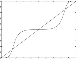
x6_{+ (1}₋_x2₎3. (3.6) The functionf(x) has the unstable fixed points ±p

1/2 and stable fixed points 0,±1 with the order of convergence to these points three, see Figure 3.2. InPublication III, the global convergence analysis for general FastICA algo-rithms with two sources can be treated in a similar way. Consider the FastICA algorithm (3.3) with symmetric orthogonalization (3.4). The changes of all the elements of matrixUin one step of iteration follow the same algorithm

x←f(x) (3.7) where f(x) =      ¯ u₁₁−u¯₂₂ √ (¯u11−u¯22)2+(¯u21+¯u12)2 , det( ¯U)<0, ¯ u11+¯u22 √ (¯u11+¯u22)2+(¯u21−u¯12)2 , det( ¯U)>0.

(28)

28 Chapter 3. Convergence of FastICA algorithms −1 −0.8 −0.6 −0.4 −0.2 0 0.2 0.4 0.6 0.8 1 −1 −0.8 −0.6 −0.4 −0.2 0 0.2 0.4 0.6 0.8 1 function y = x function wih power 3 function with power 5

Figure 3.1: Comparison of the iteration functionsf(x) in the cubic and fifth degree case

where the matrix ¯Uis the matrix after iteration (2.38) before symmetric orthog-onalization (2.42), and ¯uij are the elements of ¯U. We use two popular functions

ofg(x) to illustrate this general result. One is g(x) =x5_{, and the other one is}

g(x) = tanh(x). Figure 3.1, 3.2, and 3.3 show the function f(x) with these two nonlinearities and different source densities.

3.3 Statistical behavior of FastICA algorithms

In a practical situation, we always have finite samples. The theoretical expecta-tions are replaced by sample averages, therefore, the limit of convergence is not exactly as for the ideal case. There is a residual error due to the finite sample size. A classical measure of error is the asymptotic (co)variance of the obtained estimator. The goal of designing an ICA algorithm is then to make this error as small as possible. For the FastICA algorithm, such an asymptotic performance analysis for a general cost function was proposed in [68, 150].

S. Douglas [42, 43] gave a statistical analysis of the convergence behavior of the FastICA algorithm using inter-channel interference (ICI). The linear ICA model with the givenm-dimensional datax(n) = [x1(n)· · ·xm(n)]T, 1≤n≤N is

(29)

3.3. Statistical behavior of FastICA algorithms 29 −1 −0.8 −0.6 −0.4 −0.2 0 0.2 0.4 0.6 0.8 1 −1 −0.8 −0.6 −0.4 −0.2 0 0.2 0.4 0.6 0.8 1

Figure 3.2: Plot of the functionf(x) withg(x) = tanh(x). Boths1and

s2are binary distributed

−1 −0.8 −0.6 −0.4 −0.2 0 0.2 0.4 0.6 0.8 1 −1 −0.8 −0.6 −0.4 −0.2 0 0.2 0.4 0.6 0.8 1

Figure 3.3: Plot of the functionf(x) withg(x) = tanh(x). s1is binary distributed, s2 takes the values {−2,2} with equal probabilities 1/8, and zero with probability 3/4

(30)

30 Chapter 3. Convergence of FastICA algorithms

whereA is an unknownm×mmixing matrix, and s(n) = [s1(n)· · ·sm(n)]T is

the source. We need to find the matrixWsuch thaty(n) =Wz(n) contains the estimates of the independent sources, where z(n) = Tx(n) is the whitening of thex(n). The FastICA algorithm is

ˆ wi(k+1)= 1 N N X n=1 g(wT_ikz(n))z(n)−g′(wT_ikz(n))wik (3.9) wi(k+1)= ˆ wi(k+1) ||wˆ_i₍_k₊₁₎_|| (3.10) where the indexkmeans thekth iterative step. LetC=WTA, the inter-channel interference (ICI) is given by

ICIk = m X i=1 Pm j=1c2ijk max1≤j≤mc2ijk −1 ! (3.11) where the index k means the kth iteration step, m is the dimension of sources andcijk is the (i, j)th element of the combined system coefficient matrix.

S. Douglas [42] analyzed the behavior of the ICI and stated that all the sta-ble stationary points of the single-unit FastICA algorithm under normalization conditions correspond to the desirable separating solutions. For the two equal kurtosis sources, he states [44] that the weight vector w for the FastICA algo-rithm evolves identically to that for the Rayleigh quotient iteration (RQI) applied to a symmetric matrixΓdiag {λ1, λ2}ΓT whenΓ=PA is orthonormal, except

for the sign changes associated with the alternating update directions in the RQI. Furthermore, he conjectured that the average behavior of ICI obeyed a “1

3” rule with the nonlineartyg(y) =y3 _{[42], and proved the two-source case [44]:}

E{ICIk} ≈ 1 3 k E{ICI0}. (3.12)

InPublication II, a joint work of S. Douglas, Z.Yuan and E. Oja, the general case with kurtosis constrast function is solved. Formsources, the average ICI at iterationk is actually equal to

E{ICIk}=gm(κ1,· · ·, κm)(1

3)

k₊_R₍_{k, κ}

1,· · · , κm) (3.13)

whereκiis the kurtosis of theith source,gm(·) is a function that only depends on

the kurtoses of the sources, andR(k,·) is approximately proportional to (1/9)k

(31)

3.3. Statistical behavior of FastICA algorithms 31 0 5 10 15 −80 −70 −60 −50 −40 −30 −20 −10 0 Number of iterations k E{ICI k } [dB]

Analysis averaged over 100*100 angles FastICA simulation averaged over 10000 angles ’(1/3)’ rule averaged over 10000 angles

Figure 3.4: Evolutions of the average ICI as determined by various methods, m =4, [43].

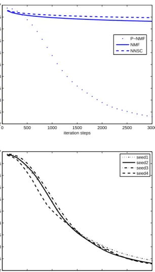
Figure 3.4 shows the actual performance of FastICA and the prediction equation (3.12) with binary source. Because of the finite data records (10000 samples), FastICA algorithm exhibits a limit E{ICIk} value. However, during its

conver-gence period, the prediction in equation (3.12) accurately describes the behavior of the FastICA algorithm.

A series of work [150, 80, 81] use Cramer-Rao lower bound (CRB) to analyze the performance of FastICA algorithms. The authors computed CRB for the demixing matrix of FastICA algorithm based on the score functions of the sources, which shows that FastICA is nearly statistically efficient. An improved algorithm called efficient FastICA (EFICA) was proposed, based on the concept of statistical efficiency. In EFICA, the asymptotic variance of the gain matrix, defined as the product of the estimated unmixing matrix and the original mixing matrix, attains the CRB which is the theoretical minimum for the variance.

(32)

32

Chapter 4

Nonnegative ICA

4.1 Nonnegative ICA algorithms

In the real world, many data have nonnegative properties. It is natural to consider adding nonnegative constraint on the linear ICA model. The combination of non-negativity and independence assumptions on the sources is refered as

non-negative independent component analysis [124, 126, 128]. Recently, Plumbley

[124, 125, 126, 127, 128] considered the non-negativity assumption on the sources and introduced an alternative way of approaching the ICA problem. Using the probability functionP r(·), he made the following definitions:

Definition 1 A sourcesis called non-negativeif Pr(s <0) = 0.

Definition 2 Anon-negativesourcesiswell-groundedif Pr(s < δ)>0for any

δ >0.

From the definition, a well-grounded non-negative sources has non-zero pdf all the way down to zero. Using these concepts, Plumbley proved the following key result [124]:

Theorem 1. Suppose that s is a vector of non-negative well-grounded inde-pendent unit-variance sourcessi, i= 1, ..., n, and y=Qswhere Q is a square

(33)

4.1. Nonnegative ICA algorithms 33

elements yj of y are a permutation of the sources si, if and only if all yj are

non-negative.

The result of Theorem 1 can be used for a simple solution of the non-negative ICA problem. The sources of course are unknown, andQ cannot be found directly. However, it is a simple fact that an arbitrary rotation ofscan also be expressed as a rotation of a pre-whitened observation vector. Denote it byz=VxwithV

the whitening matrix. Assume that the dimensionality ofzhas been reduced to that of sin the whitening, which is always possible in the overdetermined case (number of sensors is not smaller than number of sources).

It holds nowz=TAs. Because both zand shave unit covariance (for s, this is assumed in Theorem 1), the matrixTA must be square orthogonal, althoughs

andzhave non-zero means. We can write

y=Qs=Q(TA)Tz=Wz

where the matrix Wis a new parametrization of the problem. The key fact is that W is orthogonal, because it is the product of two orthogonal matrices Q

and (TA)T.

By Theorem 1, to find the sources, it now suffices to find an orthogonal matrix

W for whichy=Wz is non-negative. The elements ofy are then the sources.

This brings the additional benefit over other ICA methods that as a result we will always have a positive permutation of the sources, since both the sand y

are non-negative. The sign ambiguity present in standard ICA vanishes here. A suitable cost function for actually finding the rotation was also suggested by Plumbley [124, 126, 128]. It is constructed as follows: consider the output trun-cated at zero,y+ = (y+1, ..., y+n) withy+i = max(0, yi), and use ˆz=WTy+ as a

reestimate ofz=WT_y_{. Then we can construct a suitable cost function given by}

J(W) = E{kz₋ˆz_k2_}= E{kz₋WTy+_k2_}. (4.1) Due to the orthogonality of matrixW, this is in fact equal to

J(W) = E{ky₋y+_k2_}=

n

X

i=1

E{min(0, yi)2}. (4.2)

Obviously, the value will be zero ifWis such that all theyi are positive.

The minimization of this cost function gives various numerical algorithms [126, 128, 108, 109]. In fact, minimization of the least mean squared reconstruction

(34)

34 Chapter 4. Nonnegative ICA

error (4.1) has been proposed as an objective principle for many neural-network principal component analysis (PCA) algorithms and PCA subspace algorithms [164]. In particular, this led to the nonlinear PCA algorithm [?], whereW(t+1) =

W(t) + ∆Wwith

∆W=ηtg(y)[zT −g(yT)W] (4.3)

where g(yT) = (g(y1),· · ·, g(yn))T, and g is a nonlinear function. Algorithm

(4.3) is a nonlinear version of the Oja and Karhunen PCA subspace algorithm [107, 105], which used this algorithm withg(y) =y.The nonlinear PCA algorithm was shown to perform ICA on whitened data, ifg is an odd, twice-differentiable function [106].

Thus an obvious suggestion for our nonnegative ICA problem is the nonlinear PCA algorithm (5) with the rectification nonlinearity g(y) = y+ _{= max(}_y,_0), giving us

∆W=ηty+[zT−(y+)TW] (4.4)

which we call the nonnegative PCA algorithm. The rectification nonlinearity

g(y) = max(y,0) is neither an odd function, nor is it twice differentiable, so the standard convergence proof for nonlinear PCA algorithms does not apply. Mao [100] gave a global convergence proof of the discrete time “non-negative PCA” under certain assumptions.

In fact, the cost function (4.2) is a Liapunov function for a certain matrix flow in the Stiefel manifold, providing a global convergence [109, 100, 101].

However, the problem with the gradient type of learning rules is slow speed of con-vergence. It would be tempting therefore to develop a ”fast” numerical algorithm for this problem, perhaps along the lines of the well-known FastICA method [75]. InPublication I, we introduced such an algorithm with convergence analysis. A review is given in the following.

4.2 The nonnegative FastICA algorithm

The nonnegative FastICA algorithm, developed inPublication I, combined the nonnegative constraint and FastICA algorithm. Non-centered but whitened data

zis used, which satisfies E{(z₋E{z_})(z₋E{z_})T_}₌_I_{to keep the nonnegativity.}

A control parameter µ is added on the FastICA update rule (2.38), giving the following update rule:

(35)

4.2. The nonnegative FastICA algorithm 35

whereg− is the function

g−(y) =−min(0, y) =

−y, y <0 0, y≥0. and g′

− is the derivative of g−. This formulation shows the similarity to the classical FastICA algorithm. Substituting function g− into (4.5) simplifies the terms; for example, E{g′

−(wTz)} =−E{1|wTz <0}P{wTz< 0}, and E{(z− E{z_})g−(wTz)} = E{(z₋E{z_})(−wTz)|wTz < 0}P{wTz < 0}. The scalar

P{wTz < 0}, appearing in both terms, can be dropped because the vector w

will be normalized anyway.

In (4.5),µ is an adjustable parameter which keeps w nonnegative. It is deter-mined by:

µ= min {z:z∈∆)}

E{(z₋E{z_})wTz_|wTz<0}T_z

E{1|wT_z_<₀_}_wT_z . (4.6)

There the set ∆ ={z:zT_z_{(0) = 0}_}_{, with}_z_{(0) the vector satisfying}_||_z₍₀₎_|| _{= 1}

andwT_z_{(0) = max(}_wT_z_{). Computing this parameter is computationally}

some-what heavy, but on the other hand, now the algorithm converges in a fixed number of steps.

The nonnegative FastICA algorithm is shown below. 1. Whiten the data to get vectorz.

2. Set counterp←1.

3. Choose an initial vectorwp of unit norm, and orthogonalize it as

wp←wp− p−1

X

j=1

(wT_pwj)wj

and then normalize bywp←wp/||wp||.

4. If maxz6=0(wTpz)≤0, updatewp by−wTp.

5. If minz6=0(wpTz)≥0, updatewp bywp ←w(r)(w(r)Twp)wp, wherew(r)

is the vector in the null spacenull(Z) with Z=:{z₆= 0 :wT_pz= 0}. 6. Update wp by the equation (4.5), replacing expectations by sample

aver-ages.

(36)

36 Chapter 4. Nonnegative ICA

8. Ifwp has not converged, go back to step (4).

9. Setp←p+ 1. Ifp < nwherenis the number of independent components, go back to step (3).

4.3 Analysis of the algorithm

To analyse the convergence of the above nonnegative FastICA algorithm, the following orthogonal variable change is useful:

q=ATTTw (4.7)

whereAis the mixture matrix andTis the whitening matrix. Then

wTz=qT(TA)T(TAs) =qTs. (4.8) Note that matrixTAis orthogonal.

By theorem 1, our goal is to find the orthogonal matrix W such that Wz is non-negative. This is equivalent to find a permutation matrixQ, whose rows will be denoted by vectorsqT, such that Qsis non-negative. In the space of theq

vectors, the convergence result of the non-negative FastICA algorithm must be a unit vectorqwith exactly one entry nonzero and equal to one.

Using the above transformation in eq. (4.7), the definition of the function g−, and the parameterµ, the update rule (4.5) for the variableqbecomes

q_←µE{1|qTs<0}q₋E{(s₋E{s_})(qTs)|qTs<0}. (4.9) The idea to prove the convergence of non-negative FastICA algorithm, is to show that after each iteration, the updated vector q keeps the old zero entries zero and gains one more zero entry. Therefore, withinn−1 iteration steps, the vector

q is updated to be a unit vector ei for certain i. With total iterative steps

Pn−1

i=1 i = n(n−1)/2, the permutation matrix Q formed. The details of the proof can be found in the Publication.

It is obvious that most of the functions chosen in the classic FastICA also work in this nonnegative FastICA algorithm. However, the adjustable parameterµwill change according to the choice of the function. One exception is the function

g(y) =y, since its original function G(y) is an even and smooth function, which satisfies the requirement for the functionG(y) in FastICA. However, it can only

(37)

4.3. Analysis of the algorithm 37

find one vectorw such thatwTzis nonnegative, and therefore fails to separate the independent components.

We first make the change of variable as before fromwtoq. Sinceg(qTs) =qTs

andg′₍_qT_s_{) = 1, then the}_i_{th element of}_q_{is updated by}

qi←E{si(qTs)} −qi. (4.10)

Simplify the right-hand side of equation (4.10), note that all the sources are unit variance, we get E{si(qTs)} −qi= E{si n X j=1 qjsj)} −qi (4.11) = E{siqisi)}+ E{si n X j=1,j6=i qjsj)} −qi (4.12) = E{si} n X j=1,j6=i qjE{sj}. (4.13)

The last equation uses the fact that all the sourcessi fori= 1,· · ·, nare

inde-pendent. Then after normalization, the updated vector q does not depend on the initial data. Therefore the matrixWcannot be found.

The computation of each iteration takes more time compared to FastICA. During each iteration, the computational differences compared to classic FastICA come from step 4, 5 and 6. The step 4 is a simple value assignment. In step 5, we need to calculate the value of wT_pz once, and solve an m×n linear equation (m is the number of vectors in the source space {s₆= 0 : q(k)T_s _{= 0}_}_{). Step}

6 is the main update rule, just as in FastICA, and the extra calculation is the expectation E{z₋E{z_}}and the parameterµ. The total computation complexity takesO(N2_{) with}_N _{the number of samples, more time compared to FastICA in} each step. However, one should note that as the analysis shows above, the total number of iteration steps of our algorithm are less than or equal ton(n−1)/2.

(38)

38

Chapter 5

Nonnegative matrix

factorization

5.1 Introduction

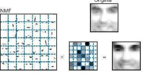
In the linear ICA model, its matrix form can be mathematically explained as the factorization of data matrixXinto two matricesAand S, whereSis the basis matrix andAis a coefficient matrix. Often the data to be analyzed is nonnega-tive, and the low rank data are further required to be comprised of nonnegative values in order to avoid contradicting physical realities. So the nonnegative con-straint is proposed on all three matrices. This new model leads to a method called Non-negative Matrix Factorization technique (NMF). Classical tools such as factor analysis and principal component analysis cannot guarantee to maintain the nonnegativity. The approach of finding reduced rank nonnegative factors to approximate a given nonnegative data matrix thus becomes a natural choice. The idea of Nonnegative matrix factorization (NMF) can be traced back to a paper of P. Paatero and U. Tapper [116] in 1994, which was named Positive matrix factorization (PMF). Suppose V is a positive m×n matrix, Paatero and Tapper advocated a positive low-rank approximationWHby optimizing the functional

min

W,H≥0||A·(V−WH)||F. (5.1) where matrix A is the weighted matrix whose elements are associated to the

(39)

5.2. The truncated singular value decomposition 39

elements of the matrix V₋WH, · denotes the Hadamard (also known as the Schur or elementwise) product. Paatero and Tapper proposed an alternating least squares algorithm (ALS) by fixing one matrix and solving the optimization with respect to the other, and reversing the matrices. Later, Paatero developed a series of algorithms [111, 112, 113] using a longer product of matrices to replace the approximantWH.

Nonnegative matrix factorization gained more applications and became popular because of Lee and Seung’s work [90, 91, 92]. Lee and Seung introduced the NMF model defined as following1_:

Given a nonnegativem×ndata matrix V, find nonnegative m×r matrix W

andr×nmatrixH with the reduced rankrsuch that the product ofWandH

minimizes

f(W,H) = 1

2||V−WH||

2_. _(5.2)

Here, W is often thought of as the basis matrix and H as the mixing matrix associated with the data inV. The measure|| · ||could be any matrix norm, or other measurements. The rankris often chosen such thatr <<min(m, n). An appropriate decision on the value ofr is critical in practice, but the choice ofr

is very often problem dependent.

Important challenges affecting the numerical minimization of (5.2) include the existence of local minima due to the non-convexity off(W,H) in both Wand

H, and perhaps more importantly the lack of a unique solution which can be easily seen by considering WDD−1H for any nonnegative invertible matrix D

with nonnegative inverseD−1_.

The objective function (5.2) of the general NMF model can be modified in several ways to reflect the application need. For example, penalty terms can be added in order to gain more localization or enforce sparsity; or more constraints such as sparseness can be imposed.

5.2 The truncated singular value decomposition

The singular value decomposition (SVD) is a classic technique in numerical linear algebra. For a given m×n matrix V, its n columns are the data items, for example, a set of images that have been vectorized by row-by-row scanning. Then

mis the number of pixels in any given image. The Singular Value Decomposition

(40)

40 Chapter 5. Nonnegative matrix factorization

(SVD) for matrixVis

V=QDRT, (5.3)

whereQ(m×m) andR(n×m) are orthogonal matrices consisting of eigenvectors ofVVT and VTV, respectively, and D is a diagonalm×mmatrix where the diagonal elements are the ordered singular values ofV.

Choosing therlargest singular values of matrixVto form a new diagonalr×r

matrix ˆD, withr < m, we get the compressive SVD matrixUwith given rankr,

U= ˆQDˆRˆT. (5.4)

Now both eigenvector matrices ˆQand ˆRhave onlyr columns, corresponding to the r largest eigenvalues. The compressive SVD gives the best approximation (in Frobenius matrix norm) of the matrixVwith the given compressive rankr

[16, 54].

In the case that we consider here, all the elements of the data matrix V are

non-negative. Then the above compressive SVD matrixUfails to keep the

non-negative property. In order to further approximate it by a non-non-negative matrix, the following truncated SVD (tSVD) is suggested. We simply truncate away the negative elements by

ˆ

U= 1

2(U+abs(U)) (5.5)

where the absolute value is taken element by element.

However, it turns out that typically the matrix ˆU in (5.5) has higher rank than

U. Truncation destroys the linear dependences that are the reason for the low rank. In order to get an equal rank, we have to start from a compressive SVD matrixUwith lower rank than the givenr. To find the truncated matrix ˆUwith the compressive rankr, we search all the compressive SVD matrices Uwith the rank from 1 tor and form the corresponding truncated matrices. The one with the largest rank that is less than or equal to the given rankr is the truncated matrix ˆU what we choose as the final non-negative approximation. This matrix can be used as a baseline in comparisons, and also as a starting point in iterative improvements. We call this method truncated SVD (tSVD).

Note that the tSVD only produces the non-negative low-rank approximation ˆU

to the data matrixV, but does not give a separable expansion for basis vectors and weights, like the usual SVD expansion.

(41)

5.3. The fundamental NMF algorithms 41

5.3 The fundamental NMF algorithms

Quite many numerical algorithms have been developed for solving the NMF. The methodologies adapted are following more or less the principles of alternating di-rection iterations, the projected Newton, the reduced quadratic approximation, and the descent search. Specific implementations generally can be categorized into alternating least squares (ALS) algorithms [116], multiplicative update al-gorithms [91, 92], gradient descent algorithm, and hybrid algorithm [122, 123]. Some general assessments of these methods can be found in [87, 151]. Actually, the multiplicative update algorithm can also be considered as a gradient descent method. Below we will briefly have a look at gradient descent methods and ALS methods.

5.3.1 NMF algorithms by Lee and Seung

One of the fundamental NMF algorithms developed by Lee and Seung [91] based on the optimal equation (5.2) with Frobenius norm is

Wia←Wia X µ Viµ (WH)iµ Haµ,Wia← Wia P jWja (5.6) Haµ←Haµ X i Wia Viµ (WH)iµ . (5.7)

In practice, a small constant 10−9_{in each update rule is added to the denominator} to avoid division by zero. Lee and Seung used the gradient descent to form the above multiplicative update algorithm by choosing the right step size. Lee and Seung [92] claimed the convergence of the above algorithm, which is not true. Lin [95, 96] pointed out their error, and proposed some modified algorithms of Lee and Seung’s method. Gonzalez and Zhang [55] presented numerical examples showing that Lee and Seungs algorithm [92] fails to approach a stationary point. Most of gradient descent methods like the above multiplicative update algorithm take a step in the direction of the negative gradient, the direction of steepest descent. Since the step size parameters of W and H vary depending on the algorithm, the trick comes in choosing the values for the stepsizes ofWandH. Some algorithms initially set these stepsize values to 1, then multiply them by one-half at each subsequent iteration [13]. This is simple, but not ideal because there is no restriction that keeps elements of the updated matrices W and H

(42)

42 Chapter 5. Nonnegative matrix factorization

algorithms is a simple projection step [140, 64, 26, 121]. That is, after each update rule, the updated matrices are projected to the nonnegative orthant by setting all negative elements to the nearest nonnegative value, 0.

5.3.2 Alternating least squares (ALS) algorithms

Another class of the fundamental NMF algorithms is the alternating least squares (ALS). ALS algorithms were first used by Paatero [116]. The basic ALS Algo-rithm for NMF is

1. InitializeWas randomm×r matrix

2. (ls) Solve forHin matrix equationWT_WH₌_WT_V_.

(nonneg) Set all negative elements inH to 0.

(ls) Solve forWin matrix equationHHTWT =HVT . (nonneg) Set all negative elements inWto 0.

3. Repeat step 2 until convergence.

In this algorithm, a least squares step is followed by another least squares step in an alternating fashion, thus giving rise to the ALS name. Although the function (5.2) is not convex in both W and H, it is convex in either W or H. Thus, given one matrix, the other matrix can be found with a simple least squares computation [86].

In the above algorithm, a simple projection step, which sets all negative elements resulting from the least squares computation to 0, is used to keep nonnegativity. This simple technique also has a few added benefits. Of course, it aids sparsity. Moreover, it allows the iterates some additional flexibility not available in other algorithms, especially those of the multiplicative update class. One drawback of the multiplicative algorithms is that once an element inW or H becomes 0, it must remain 0. This locking of 0 elements is restrictive, meaning that once the algorithm starts heading down a path towards a fixed point, even if it is a poor fixed point, it must continue in that vein. The ALS algorithms are more flexible, allowing the iterative process to escape from a poor path.

Depending on the implementation, ALS algorithms can be very fast. The im-plementation shown above requires significantly less work than other NMF al-gorithms and slightly less work than an SVD implementation. Improvements to the basic ALS algorithm appear in [113, 87].

Advances in independent component analysis and nonnegative matrix factorization

ADVANCES IN INDEPENDENT COMPONENT

ANALYSIS AND NONNEGATIVE

MATRIX FACTORIZATION

ABSTRACT

Preface

Contents

List of symbols

List of abbreviations

Chapter 1

Introduction

1.1

Motivation and overview

1.2

Contributions of the thesis

1.3

Publications of the thesis

Chapter 2

Independent component

analysis

2.1

Linear ICA model

2.2

Data preprocessing for ICA

2.2.1

Principal component analysis (PCA)

2.3

Measuring the independence

2.3.1

Uncorrelation and whitening

2.3.2

Entropy and cumulants

2.3.3

Mutual information

2.4

ICA algorithms

2.4.1

Algorithms by maximum likelihood

2.4.2

Tensorial methods

2.5

FastICA

Chapter 3

Convergence of FastICA

algorithms

3.1

Local convergence

3.2

Global convergence

3.3

Statistical behavior of FastICA algorithms

Chapter 4

Nonnegative ICA

4.1

Nonnegative ICA algorithms

4.2

The nonnegative FastICA algorithm

4.3

Analysis of the algorithm

Chapter 5

Nonnegative matrix

factorization

5.1

Introduction

5.2

The truncated singular value decomposition

5.3

The fundamental NMF algorithms

5.3.1

NMF algorithms by Lee and Seung

5.3.2

Alternating least squares (ALS) algorithms