The use of CMIP5 data to simulate climate change impacts on flow regime within the Lake Champlain Basin

ContentslistsavailableatScienceDirect

Journal

of

Hydrology:

Regional

Studies

jo u r n a l h o m e p a g e :w w w . e l s e v i e r . c o m / l o c a t e / e j r h

The

use

of

CMIP5

data

to

simulate

climate

change

impacts

on

flow

regime

within

the

Lake

Champlain

Basin

Ibrahim

Nourein

Mohammed

,

Arne

Bomblies

,

Beverley

C.

Wemple

a_{UniversityofVermont,EPSCoR,23MansfieldAve,Room208A,Burlington,VT05401,USA}

b_{UniversityofVermont,DepartmentofCivilandEnvironmentalEngineering,221VoteyHall,Burlington,} VT05405,USA

c_{UniversityofVermont,DepartmentofGeography,208OldMill,Burlington,VT05405,USA}

a

r

t

i

c

l

e

i

n

f

o

Articlehistory: Received4July2014

Receivedinrevisedform7January2015 Accepted18January2015

Availableonline24March2015 Keywords:

Hydrology Streamflow Climateimpacts

Climatechangeandvariability Ecologicalprediction Ecosystems

a

b

s

t

r

a

c

t

Studyregion:LakeChamplainBasin,northwesternNewEngland,USA. Studyfocus:Ourstudyusesregionalhydrologicanalysesandmodelingto exam-inealternativepossibilitiesthatmightemergeintheLakeChamplainBasin streamflowregimeforvariousclimatescenarios.Climatedataaswellas spa-tialdatawereprocessedtocalibratetheRegionalHydro-EcologicalSimulation System (RHESSys) model runoff simulations. The 21st century runoff simulations wereobtainedbydrivingtheRHESSysmodelwithclimatedatafromtheCoupled ModelIntercomparisonProjectphase5(CMIP5)forrepresentativeconcentration pathwaysRCP4.5and8.5.

Newhydrologicalinsightsfortheregion:Ouranalysessuggestthatmostof CMIP5ensemblesfailtocaptureboththetrendsandvariabilityobservedin his-toricalprecipitationwhenruninhindcast.Thisraisesconcernsofusingsuch productsindrivinghydrologicmodelsforthepurposeofobtainingreliablerunoff projectionsthatcanaidresearchersinregionalplanning.Asubsetoffive cli-matemodelsamongtheCMIP5ensembleshaveshownstatisticallysignificant trendsinprecipitation,butthemagnitudeofthesetrendsisnotadequately repre-sentativeofthoseseeninobservedannualprecipitation.Adjustedprecipitation forecastsprojectastreamflowregimedescribedbyanincreaseofabout30%in seven-daymaximumflow,afourdaysincreaseinfloodeddays,athreeordersof magnitudeincreaseinbaseflowindex,anda60%increaseinrunoffpredictability (Colwellindex).

©2015TheAuthors.PublishedbyElsevierB.V.Thisisanopenaccessarticle undertheCCBY-NC-NDlicense (http://creativecommons.org/licenses/by-nc-nd/4.0/).

∗Correspondingauthor.Tel.:+18026567351;fax:+18026562950.

E-mailaddresses:[email protected](I.N.Mohammed),[email protected](A.Bomblies), [email protected](B.C.Wemple).

http://dx.doi.org/10.1016/j.ejrh.2015.01.002

2214-5818/©2015TheAuthors.PublishedbyElsevierB.V.ThisisanopenaccessarticleundertheCCBY-NC-NDlicense (http://creativecommons.org/licenses/by-nc-nd/4.0/).

1. Introduction

Overthepastseveraldecades,temperatureandprecipitationhaveincreasedsignificantlyinthe northeasternUnitedStates(Hayhoeetal.,2007,2008;Huntingtonetal.,2009;Melilloetal.,2014). Understandingtheimpactsoftheseclimaticchangesonwatershedhydrologyisimportantforhuman societyandecologicalprocesses.However,theobservedclimatetrendsshowsignificantspatial vari-ability withinNew England in additionto pronouncedseasonality (Hayhoe etal., 2008).Recent disseminationofdownscaledGlobalCirculationModel(GCM)datahasmadesuchregionalanalysis tractable.Forexample,statisticallydownscaleddataproductssuchastheCoupledModel Intercom-parisonProject(CMIP5)multi-modelensembleanditspredecessorsarecommonlyappliedasdrivers ofhydrologymodels(Meehletal.,2007;Tayloretal.,2011;Meehletal.,2014).Suchdownscaleddata havegreatpotentialtoaidresearchers,resourcemanagers,andotherpolicymakersinthe assess-mentofclimatechangeimpactsonwaterandtheenvironment.However,atleasttwostudieshave documentedpoorcorrelationbetweenprecipitationobtainedfromsuchdownscaledclimatemodel productsandobservations(Stephensetal.,2010;vanHarenetal.,2013),thereforetheapplicability ofCMIP5precipitationdataforregionalhydrologicalimpactsanalysismustbevalidated.

ChangesinstreamflowregimeinthenortheasternUnitedStateshavebeenexaminedinmultiple studiesusinghistoricaldatasets(HartleyandDingman,1993;Hodgkinsetal.,2003,2005;Hodgkins

andDudley,2005,2006;Campbelletal.,2011).Theseworkssummarizedtheobservednortheastern

streamflowregimechangeastimingshifttowardearlierspringflowandamoreuniformdistribution offlowthroughoutthesnowmeltperiod(i.e.,Marchstreamflowshaveincreased,whileMayflows havedeclined).However,summerbaseflowincreasedinundammedNewEnglandriversduringthe latterhalfofthetwentiethcentury(HodgkinsandDudley,2011).

Potentialimpactsofclimaticchangesonaquaticecosystemsspecies,nutrientdelivery, tempera-turesandhydrologyhavebeendiscussedfordifferentregionsoftheUnitedStates(Melacketal.,1997;

Haueretal.,1997;Mulhollandetal.,1997;Mooreetal.,1997;Stoneetal.,2001).Naturalflowregime

playsamajorroleinsustainingnativebiodiversityandecosystemintegrityinrivers(Poffetal.,1997). Streamflowregimealterationmayalsoaffectaquaticorganisms,sedimentmovementandfloodplain interactions(Gibsonetal.,2005).Characterizationofflowregimehasbeenexaminedviametricsthat describethemagnitude,frequency,duration,timingandrateofchangeforstreamflow(Poff,1996;

Poffetal.,1997;Puckridgeetal.,1998).Thesestreamflowmetricsareusefuldeterminantsof

ecolog-icalprocessregulationinriverecosystems.Numeroussimilarstreamflowregimemetricshavebeen compiled(Richteretal.,1996;Puckridgeetal.,1998;SnelderandBiggs,2002).

TheLakeChamplainBasinisamulti-stateandbi-nationalwatershed(Vermont,NewYorkand Québec)withadrainageareaofabout21,000km2 _{(Stagerand Thill,2010)andservesasamajor} sourceofecosystemservicesandeconomicinputstothenortheasternUnitedStates.Predicted21st centuryclimaticchangesareexpectedtoimpactarangeofenvironmentalprocessesintheBasinand thereforeraiseconcernsabouthydrological,ecologicalaswellaspoliticalconditions(StagerandThill, 2010).Therefore,anevaluationofclimatechangeimpactsonregionalhydrologywouldgreatlybenefit policymakersandotherstakeholders.Inthisstudy,weexaminethereliabilityoftheCMIP5ensemble ofsimulationsinperformingregionalhydrologicalimpactsanalysisinnorthwesternNewEngland.We alsodiscusstheuncertaintyassociatedwithclimatechangeimpactsonaVermontwatershedflow regime.WeperformsuchanassessmentintheMadRiverwatershedofVermont,andsubsequently predictfutureflowregimefortheMadRiverusingthedownscaledclimatedatausingmetricsthatare usefultopolicymakersandecologists.

2. Methods 2.1. Studyarea

TheMad RivernearMoretownis a 360km2 _{tributarywatershed of theWinooskiRiver(HUC} 02010003)withintheVermontportionoftheLake Champlainbasin (Fig.1).Thiswatershedisa representativestudyareaforexaminingtheimpactsofclimatechangeonstreamflowregimesince themixedforested,agriculturalandvillagecenterlandcoversaretypicaloftheVermontlandscape.

Fig.1. MadRivernearMoretownwatershed(USGS#04288000)islocatedwithintheWinooskibasin(HUC02010003).The watersheddrainageareaisabout360km2_{.TheheadwateroftheMadRiverisGranvilleNotchFalls.MadRiverdrainsintothe} WinooskiRiverwhichinturndrainsintoLakeChamplain.

Thewatershedismainlyforestedwithurbanizedtowncenters(about4%ofwatershedarea)and agriculturallands(about8%ofwatershedarea)foundmainlyonthevalleyfloor.

AlongmonitoringstreamflowdatarecordisavailablefortheMadRiverwatershedatitsoutlet.The watershedoutlet(UnitedStatesGeologicalSurvey(USGS)streamflowgauge#04288000)islocated at44◦1638Northand72◦4435West(referencedtotheNorthAmericanDatum(NAD)of1927) withintheWashingtonCounty,Vermont.Thegaugealtitudeis170mabovesealevelreferenced totheNationalGeodeticVertical Datum(NGVD)of1929.TheMadRiverflowsnorthtowardthe WinooskiRiver,whichflowstoLakeChamplain.LakeChamplainisdrainedbytheRichelieuRiverto thenorthandissituatedwithintheSt.LawrenceRiverdrainage.ThestreamflowrecordattheMad RivergaugebeginsinOctober1928.StreamflowdataforthisworkwasretrievedfromtheUSGSportal

(http://waterdata.usgs.gov/nwis/dv/?site no=04288000&agency cd=USGS&referred module=sw)

accessedon4February2014.Meanannualrunoff(Q)measuredattheoutletofthestudywatershed duringtheperiod1950–2013(wateryears)is714mm.Aprilisthehighestyieldmonthatthe water-shedoutletwithmonthlymedianrunoffof160mm,andindriermonths,occasionalfluctuationsat lowflowhaveoccurred.Meanannualprecipitation(Pcp)onthestudywatershedis1235mm.Table1

showstheannualmeanprecipitation,runoff andevapotranspiration(E)fortheyears1920–2010 overthestudywatershed.Theannualaverageevapotranspirationwascalculatedusingmassbalance (E=Pcp−Q).

2.2. Spatialdata

Adigitalelevationmodel(DEM)with30mgridresolutionforthestudyareawasobtainedfromthe NationalElevationDataset(NED)portal(http://seamless.usgs.gov/website/seamless/viewer.htm)and wasusedtoderiveslopeandaspectgridsforthemodelinput.Fig.2,panel(a)showsthetopography ofourstudywatershed,whichrangesfrom170to1240mabovesealevelwithameanvalueof491m. LanduseandvegetationdatawereobtainedfromtheNationalLandCoverDataset(NLCD2006)

(http://gisdata.usgs.net/website/MRLC/viewer.htm).We grouped vegetationand land usefor our

studywatershedintoeightcategories:coniferousforest,deciduousforest,mixedforest,grassland, novegetation,shrub,agricultureandurban.Theforestcoverdominatesabout87%ofthewatershed area(52%deciduous,23%mixed,and12%coniferforests).Thereareafewagriculturallandsandsmall urbanareaswithinvalleysandscatteredoverthewatershedarea(Fig.2,panelb).

ThewatershedsurfacesoiltexturemapwasobtainedfromtheNaturalResourcesConservation ServiceCountySoilSurveyData datasetthroughtheVermontCenterforGeographicInformation Gateway(http://vcgi.vermont.gov/).CountysoildatafortheWashington,AddisonandChittenden countieswereobtainedtocompileourwatershedsoiltexturemap.Thewatershedsoiltextureis mainlysandyclayloam(approximately80%ofthewatershedarea)whichhas34%claycontent.The meansoildepthatthevalleyfloorisapproximately1.5m.

2.3. Climatedata

Daily precipitation (Pcp), minimum and maximum air temperatures (Tmin and Tmax), and

windspeed(w)datawereobtainedfromtheSantaClara Universityportal(http://www.engr.scu.

edu/emaurer/data.shtml)(Maureretal.,2002).Thedataisatdailyand1/8th_{degreeresolutionsfor}

theperiod1January1949to31December2010,andconstitutesthehistoricalclimatedatasetforour

Table1

MadRivernearMoretown,Vermont(USGS#04288000)annualwaterbalanceestimates(1950–2010).Precipitation(Pcp)from Maureretal.(2002),Runoff(Q)fromtheUSGSnationalwaterinformationsystem(http://waterdata.usgs.gov/nwis)gauge number04288000.Meanannualevapotranspirationestimatedfrommassbalance.

Variable Minimum 25th_{percentile Median Mean 75}th_{percentile Max}

Pcp(mm) 851 1091 1198 1235 1361 1805

Q(mm) 332 579 671 682 786 1074

Fig.2. Spatialinputdata.(a)Digitalelevationmodel(DEM)(30mgridsize)and(b)landcover.Landcoverdataarefromthe NLCD2006dataset.

study.TheclimaticseasonalvariationforourstudywatershedisshowninFig.3.Julyisthehottest monthoftheyearwithaveragedailymaximumandminimumair temperaturesof24 and13◦C respectively.

OutputdatafromtwoscenariosofRepresentativeConcentrationPathways(RCP4.5and8.5) sim-ulationsofGCMoutputdata(dailyprecipitation,minimumandmaximumairtemperatures)were obtainedfromtheCoupledModelIntercomparisonProjectphase5(CMIP5)multi-modelensemble

(Tayloretal.,2011).Thegriddeddatasetsareallat1/8th _{degreeresolution,andaggregatemetrics}

forprecipitation(Pcp)andairtemperatures(TminandTmax)werecalculatedfortheeightgridcells

spanningtheMadRiverwatershed.

Downscaledmodelinputsselectedwerethebiascorrectionconstructedanalogsmethod(BCCA) productsdiscussedbyMaureretal.(2010).FulldetailsabouttheclimatescenariodataareinBrekke

etal.(2013).Forthiswork,weutilizedthegriddedbias-corrected climatescenarios datafor the

2006–2100timeperiodaswellastheretrospectiveclimatedatafor1951–2005timeperiod(further detailsonclimatemodelscanbefoundatAppendixA).

A visualassessment of the CMIP5 projection ensembleshindcast data when compared with observedhistoricprecipitation(Maureretal.,2002)suggeststhattheCMIP5modelensembleshave poorlycapturedthevariabilityandtrendshistoricallyobserved.Fig.4showstheannualobserved precipitationtimeseriesoverthestudywatershedduring1951–2005wateryearsalongwiththe twenty-oneCMIPensembleswhenrunonahindcastmode.

Figs.5and6showannualprecipitationandannualairtemperatures(minimumandmaximum),

respectively,aggregatedoverourstudywatershedfromtheCMIP5subsetensemblesundertheRCP8.5

scenario.Thereisalargedifferenceintheslopebetweenhistoricalandfutureprecipitationprojections.

2.4. RHESSysmodeldescription

TheRegionalHydro-EcologicSimulationSystem(RHESSys)modeldescribedbyBandetal.(1993,

0 50 100 150 200 250 300

Jan Feb Mar Apr May Jun Jul Aug Sep Oct Nov Dec

Runoff (mm) 0 50 100 150 200 250 300 Precipitation (mm) 3 4 5 6 7 8 Wind speed (m/s) −20 −10 0 10 Min Temperature (°C) −10 0 10 20 Max Temperature (°C)

Fig.3. HistoricclimateinputdataoverthestudywatershedandmeasuredrunoffattheMadRivernearMoretownwatershed outlet(USGSgauge#04288000)during1949–2010.Boxplotsofmonthlyaveragesofminimum,maximumairtemperatures andwindspeed.Boxplotsofprecipitationandrunoffamountssummedmonthly.ClimatedataobtainedfromMaureretal. (2002).

Fig.4. AnnualhistoricprecipitationaggregatedovertheMadRivernearMoretownwatershed(USGSgauge#04288000)during 1951–2005wateryears.ObserveddataobtainedfromMaureretal.(2002)depictedassolidblackline(Maurer),whileclimate dataoftwentyoneclimatemodels(runonhindcast)wereobtainedfromtheCoupledModelIntercomparisonProjectphase5 (CMIP5)ensembles(http://gdo-dcp.ucllnl.org/downscaledcmipprojections/dcpInterface.html).

(mm)

Fig.5. Annualprecipitationaggregatedover theMadRivernearMoretownwatershed(USGSgauge#04288000). His-toricalclimatedataobtained fromMaureretal. (2002), whilescenario(RCP8.5)climatedata offiveclimatemodels wereobtainedfromtheCoupledModelIntercomparisonProjectphase5(CMIP5)ensembles(http://gdo-dcp.ucllnl.org/ downscaledcmipprojections/dcpInterface.html).

tosimulatecarbon,waterandnutrientfluxes.RHESSyscombinesbothasetofphysicallybasedprocess modelsandamethodologyforpartitioningandparameterizingthelandscapeoverspatiallyvariable terrainrangingfromtenmeterstohundredsofkilometers.TheversionofRHESSys usedforthis work(5.14.4)includesbothsurfaceandsubsurfacestorageroutingandadeepgroundwaterstore

(Tagueetal.,2008).TheRHESSysmodelisabletosimulateinteractionsbetweencarbon,waterand

nutrientfluxesandclimatepatternswithinamountainousenvironment.Waterisexplicitlyrouted betweenspatialpatches,representingspatialheterogeneityinsoilmoistureandlateralwaterflux tothestream.TheRHESSyshydrologicprocessmodelshavebeenadaptedfromseveralpre-existing

Mini

m

um

°

C

Maxi

m

um

Fig.6. AnnualminimumandmaximumairtemperatureaggregatedovertheMadRivernearMoretownwatershed(USGS gauge#04288000).Historicalclimatedataobtained fromMaureretal.(2002),whilescenario(RCP8.5)climatedata of fiveclimate models were obtained from the Coupled ModelIntercomparison Project phase 5(CMIP5) ensembles (http://gdo-dcp.ucllnl.org/downscaledcmipprojections/dcpInterface.html).Maureretal.dataaredepictedinredandblue colorsformaximumandminimumairtemperaturesrespectively.

modelsandtheyincludesnowaccumulationandmelt,interception,infiltration,transpiration,soil andlitterinterception,evaporationandshallowanddeepgroundwatersubsurfacelateralflow.Most processesarerunatadailytimestep.

Forthiswork,weusedtheroutingapproachadaptedfromtheDistributedHydrologySoiland Vege-tationModel(DHSVM)(Wigmostaetal.,1994)toroutethewaterlaterally.TheDHSVMroutingmodel simulatessaturatedsubsurfaceinterflowandoverlandflowviapixel-by-pixelbasisconnectivity.An importantmodificationfromthegrid-basedroutingofDHSVMistheabilityofRHESSystoroutewater betweenarbitrarilyshapedsurfaceelements.Thisallowsgreaterflexibilityindefiningsurfacepatches andvaryingshapeanddensityofsurfacetessellation.Thenareasonableapproximationofrealityin simulatinglateralmoistureroutingatthelevelofspatialdataresolutionemployedisachieved.

RHESSyspartitionsthelandscapeintodistributedelementshierarchicallyorganizedintobasin

(watershed),zone,hillslope,patchandstratum.Inthiswork,zonesrepresentingclimateinformation havebeenpartitionedfollowingthe1/8th_{degreeclimategridfromMaureretal.(2002).Thereare} eightdifferentzonesspanningourstudywatershed.Hillslopesweregeneratedusingthewatershed analysisroutine(r.watershed)inGRASS(GRASSDevelopmentCoreTeam,2012)withcontributingarea thresholdof21,600m2_{resultingin16,560hillslopes.Weobtainedthestreamnetworkcontributing} areathresholdobjectivelyfromastreamdroptestfollowingtheorydescribedinTarbotonetal.(1991,

1992).Eachhillslopewastreatedasasinglemodelelement(i.e.,patch).Stratumisusedforcanopy

informationandinheritsthepatchspatialsetting(i.e.,hillslopeinthiswork).

RHESSysusestheMountainMicroclimateSimulator(MTN-CLIM)model(Runningetal.,1987)to obtainspatiallyvariableclimateinputs.Dailyclimatedataofminimumandmaximumairtemperature aswellasprecipitationdriveRHESSysfluxestimates.TheMTN-CLIMmodelsimulatesradiation, par-titioningofrainandsnow,saturationvaporpressure,andrelativehumidity.MTN-CLIMextrapolates meteorologicalvariablesfromthepointofmeasurementstothemodelingunitofinterest(hillslope) makingcorrectionsfordifferencesinelevation,slopeandaspectbetweenthepointofmeasurements andtargets(hillslopes).Lapseratesusedinthisworktoadjustairtemperaturesanddewpointspatially are0.01and0.0015◦C/m,respectively.

Canopyheightsandspeciesspecificvegetationparameters(MyersandEdminster,1972;Kaufmann

Table2

Streamflowregimevariablesusedtoexamineclimatechangesimpacts.

Variablename Symbol Definition Streamflowclassification

Dailymeandischarge QMEAN Averagedailyflowovera

wateryear

Staticbasindescriptor

Highflowdisturbance Q1.67 Flowofmagnitudeexceedinga

returnintervalof1.67years basedonalog-normal distribution

Highflowdisturbance

Floodduration FLDDUR Theaveragenumberofdays

peryearwhenflowequalsor exceedsQ1.67

7daymaximumflow 7QMAX Theaverageannualmaximaof

7daymeansofdailymean streamflow

Baseflowindex BFI Theratiooftheannuallowest

dailyflowtotheaveragedaily flowmultipliedby100during awateryear

Lowflowdisturbance

7dayminimumflow 7QMIN Theaverageannualminimaof

7daymeansofdailymean streamflow

Coefficientofvariation DAYCV Theratioofthestandard

deviationofdailyflowstothe averageofdailyflows multipliedby100duringa wateryear

Flowvariabilityand predictability

Flowreversal R Theaveragenumberofdaily

flowreversalsperyear

ColwellindexofPredictability P Predictabilityofflowusinganindex developedbyColwell(1974)whichis basedoninformationtheory ColwellindexofConstancy C

ColwellindexofContingency M

RHESSyslibraries.Thesixvegetationcategoriesgroupedforthestudywatershedwerelinkedwith vegetationparametersfromRHESSyslibraries.

Initialleafareaindex(LAI)valuesatthehillslopelevelforourstudywatershedwerefoundby reclassifyingspecificvegetationclasseswithLAIvalues.LAIvaluesforeachvegetationclassusedfor reclassificationwereobtainedfromWhiteetal.(2014)andsuggestedliteratureoverthestudyregion

(Dingman,2002,Table7–5).TheaggregateaverageLAIoverthestudywatershedisabout4.6.

RHESSysusesmanyparameterstodescribetypicalsoil,vegetationandlandusecharacteristics. Literature-basedestimateshavebeenusedtocompileparametersforcommonvegetationandsoil types.CalibratedparameterswithinRHESSysare(1)thedecayofhydraulicconductivitywithdepth (m),(2)saturatedsoilhydraulicconductivityatthesurface(k),(3)thefractionofrechargethatbypasses theshallowsubsurfaceflowsystemtodeepergroundwaterstorage(gw1),and(4)thedrainagerate ofdeepergroundwaterstore(gw2).

2.5. Flowregime

Inthispaper,weexaminethreestreamflowclassesandhowtheychangewithclimateattheMad RivernearMoretownstreamflowgauge(watershedoutlet).Thestreamflowclassesstudiedarehigh flowdisturbance,lowflowdisturbanceandflowvariabilityandpredictability(Table2).

Highflowdisturbancestreamflowmetricsincludethreestreamflowvariables:ahighflow disturb-ancevariable(Q1.67),afloodduration(FLDDUR)variable,andaseven-daymaximumflow(7QMAX) variable.DunneandLeopold(1978)definebankfullstageas“thestagethatcorrespondstothe dis-chargeatwhichchannelmaintenanceisthemosteffective,thatis,thedischargeatwhichmoving sediment,formingorremovingbars,formingorchangingbendsandmeanders,andgenerallydoing

workresultsintheaveragemorphologiccharacteristicsofchannel.”WolmanandMiller(1960) con-cludedthatthebankfullstageisthemosteffectiveoristhedominantchannelformingflow.Thereisa wideagreementthatonaverageabankfullflowhasanaveragerecurrenceintervalof1.5years,

how-everPoff(1996)andChinnayakanahallietal.(2011)citethataflowwitha1.67yearreturnintervalis

oftenrecognizedasbankfullflow.TheQ1.67flowisdefinedasaflowofmagnitudeexceedingareturn intervalof1.67yearsbasedonfittingalog-normalprobabilitydistributiontotheannualmaximum dailyflowseriesthenselectingthevaluethathasaprobabilityofexceedanceof1/1.67(Dunneand

Leopold,1978).Historicalstreamflowdata(1955–2013wateryears)atthestudywatershedgauge

suggestthatQ1.67forthestudygaugeisabout24millimeterperday(3,587cfs).Floodduration( FLD-DUR)isusuallycalculatedastheaveragenumberofdaysperyearwhenflowequalsorexceedsQ1.67

flow.Forthehistoricalstreamflowperiodstudied,themeanflooddurationforthestudywatershed usingareturnflowof24mm/dayislessthanoneday.

Since the Mad River watershed is flashy, estimating the magnitude of daily return flow that we can use in calculating flood duration periods is quite challenging (floods last only several hours). The National Weather Service (NWS) flood stage guidelines at our watershed

(http://water.weather.gov/ahps2/hydrograph.php?wfo=btv&gage=moov1),accessedon26February

2014,indicatethatninefeetisthethresholdstageforfloodwarning.WethustaketheMadRiver nearMoretownstreamflowgaugebankfullstageasninefeet.Weextractedallthedayswhenstageat ourwatershedwasequaltoorexceeded9feetfromthehistoricalinstantaneouscrestsrecordduring 1927–2013providedbytheUSGS.Theinstantaneousfloodpeakflowsvaryfromfourto166mm/day (i.e.,530–24,300cfs).Weexaminedthedailyrunoffvaluesatthesefloodeddays.Wefoundthatthe dailyrunoffatthesefloodeddaysvariesfromabout1to44mm/day(i.e.,160–6,140cfs)with25th percentileat15mm/day(2,175cfs)and50th_{percentileat24mm/day(3,575cfs).Mappinghistorical} crestdataondailyflowdataismorerealisticintermsofcapturingflooddurationratherthanjust relyingontheQ1.67discussedearlier.Thethresholdusedtocalculateflooddurationperiodsforthis workwassetas15mm/day(25th_percentile).

Asimplewaytodepictadistributionistoexamineahistogram.Ahistogramcountsthe num-berofoccurrenceswithinpredefinedbins.However,identifyingmodesfromthehistogramrequires visualinterpretationandissomewhatsubjectivebecauseofthechoiceofbinwidth.Silverman(1986)

presentednonparametricdensityestimationmethodsthatcandepictthedistributionofdatamore generallyandobjectively.Kernelmethodsarepopularnonparametricapproachesthatwehaveused heretoshowdifferentfloodscenarios.Thekernelmethodsaremostsensitivetotheselectionof band-width(h).Therearemultiplemethodsthatgiveestimatesforthebandwidth(h)(Silverman,1986;

SheatherandJones,1991;Scott,1992).HereweusedtheSheatherandJonesmethodimplemented

bytheRstatisticalsoftwarepackagetoselectbandwidth(h)(RDevelopmentCoreTeam,2014)anda Gaussianfunctionforthekernel.

Seven-daymaximumflow(7QMAX)istheaverageacrossyearsof7-daymaximumstreamflow.For eachyearintheperiodofrecord,themaximum7-daymeanisfoundfromthedailymeanstreamflow andthemaximumisthe7-daymaximumflowforthatyear.A7QMAXistheaverageofthoseyearly 7-daymaximumvaluesandforthehistoricaldata;itisabout10millimetersperday(1,513cfs).

Lowflowdisturbancestreamflowmetricsincludeabaseflowindexforameasureofchangesin baseflow (BFI)variableanda7-dayminimum(7QMIN)variable.Baseflow index(BFI)istheratio oftheannuallowestdailyflowtotheaverageflowmultipliedby100.BFIisalowflowvariablethat indexesflowstabilityandsusceptibilitytodrying.Historicalstreamflowdatasuggeststhatthemedian ofBFIatthestudygaugeisabout9%.Seven-dayminimumflow(7QMIN)variableistheaverageacross yearsof7-dayminimumstreamflow.Foreachyearintheperiodofrecord,theminimum7-daymean isfoundfromthedailymeanstreamflowandtheminimumisthe7-dayminimumflowforthatyear. A7QMINistheaverageofthoseyearly7-dayminimumvaluesandforthehistoricaldata;itisabout onemillimeterperday(199cfs).

Flowvariabilityandpredictabilitystreamflowmetricsincludeacoefficientofvariation(DAYCV) variable,aflowreversal(R)variableandthreeflowvariablesdefiningtheColwellindexwhichare Predictability,ConstancyandContingency(Colwell,1974).Flowreversaleventsareoftenrelated tophysicaldisturbanceinstreamecology(Reshetal.,1988).Streamflowvariabilityexertscontrol overmanyimportantstructuralattributesinstreams(e.g.,habitatvolume,currentvelocity,channel

geomorphology,andsubstratumstability).Temporalpatternsofstreamflowareimportantin the fluctuatingphysicalandbiologicalenvironmentofrivers(Lazzaroetal.,2013).

Coefficientofvariation(DAYCV)isthestandarddeviationofdailyflowsdividedbytheaverage ofdailyflowsmultipliedby100duringayear.TheDAYCVdescribesoverallflowvariabilitywithout consideringthetemporalsequenceofflowvariation.HistoricaldatasuggeststhatthemedianofDAYCV

atthestudywatershedisabout137%,whichsuggestsahighrateofstreamflowchange(flashiness). Flowreversals(R)aredefinedfromthedailymeanstreamflowasdayswhenthetrend(increasing ordecreasing)fromthepreviousdaysisreversed.Historicalstreamflowdatafromthestudygauge givesthemedianofRasabout125days.

Flowpredictabilitymetricsweredeveloped(Colwell’sindices,Colwell,1974)toassessbiologically relevantmeasuresofflowvariability.TheprincipalvalueoftheColwellindexusedinourworkisfor comparisonoftheuncertaintyofthevariableriverenvironmentprojectedinfuture.TheColwellindex isalsousefulfortheassociationofnaturalvariationinflowregimewithaquaticmacroinvertebratetaxa richnessandcompositionwithintheecologicalcommunity(PoffandWard,1989;Chinnayakanahalli etal.,2011).Streamecologistsareofteninterestedinthistheorybecauseofthegreattemporal vari-abilitywithinandbetweenriverecosystemenvironments.Colwell(1974)procedureisanalogousto autocorrelationanalysisandtosomeaspectsofharmonicanalysis.TheColwell’spredictability(P)is thesumofconstancy(C)andcontingency(M).Constancy(C)isameasureoftemporalinvariance,and contingency(M)isameasureofperiodicity.Constancyisdefinedsimilartopredictability,exceptthat seasonalvariabilityacrossperiodsisdisregarded.Contingencyisdefinedasthedegreetowhichtime periodandvaluegrouparedependentoneachother.TheP,C,andMarescaledtorangefrom0to1 (furtherdetailsonColwellindexarepresentedatAppendixB).

CalculationofColwell’sindicesrequiresthatstreamflowvaluesbebinnedintodiscretegroups. Aswithallinformationmeasuresabsolutevaluesaredependentonthisbinning,butaconsistent binningallowsrelativecomparisons.FollowingGordonet al.(2004)andChinnayakanahallietal.

(2011),weused7bins(<0.5,1.0,1.5,2.5,3.0,>3.0),whereisequaltothemeanof

dailystreamflowvalues,todefinegroupsforeachmonth.Weusedtwelvemonthstorepresentthe seasonalcycleandcountedthenumberofoccurrencesofdailystreamflowvaluesinstatesdefinedby groups(bins)andperiods(months).AnalysisoftheMadRiverwatershedhistoricalstreamflowdata (1955–2013wateryears)usingthesemetricsindicatesthattheflowhasalowpredictability(P_≈0.25) TheConstancy(C)attheobservedhistoricalpredictabilityis0.23.FishspeciesobservedattheMad Rivermouth(i.e.,warmwaterfishhabitat)areBrooktrout,Longnosedace,andSlimysculpin.Weinfer thattheobservedlowColwell’spredictabilitycalculatedissuitabletomaintaintheabove-mentioned species.

3. Results

3.1. Modelcalibrationandverification

Inthiswork,themodelwascalibratedtodailystreamflowsatthewatershedoutletduringthree dif-ferentwateryears(wet,averageanddry)inordertoassessmodelperformanceoverarangeofclimatic conditions.Thewetwateryearselectedformodelcalibrationhasannualprecipitationof1445mm. MonteCarlosimulationwasusedtogenerate5500sampleparametersetsfromindependentuniform distributionsoverthefeasibleparameterrangesdeterminedfromtheliteraturerangesform,k,gw1, andgw2parameters.Eachsampleparametersetwasusedasaninputtothemodel,andmodel per-formancewasassessedusingtheNash–Sutcliffeefficiencymetricondailyflows(NS),Nash–Sutcliffe efficiencymetriconlogdailyflows(NSlog)andtotalannualflowerror(Qerr).Werepeatedthisstep fortheremainingselectedwateryears(averageanddry)andresultswereshowninFig.7(average wateryear).Wenotethatmodelresultsweremoresensitivetochangesinvaluesofgw1andgw2

parametersthantochangesintheotherparameters.Thesaturatedsoilhydraulicconductivityatthe surface(k)parameterdepictedinFig.7isamultiplierofhydraulicconductivityatthesurfaceforboth soiltexturetypesusedinthewatershedsoiltexturemap(sandyclayloamsoilhydraulicconductivity atthesurfaceusedwasabout0.544m/day,whileclayhydraulicconductivityatthesurfaceusedwas about0.111m/day).

0 5 10 15 20 25 0.0 0 .2 0.4 0 .6 0. 8 m (meter) NSE 0 1 2 3 4 5 0.0 0 .2 0.4 0 .6 0. 8 k NSE 0 20 40 60 80 100 0.0 0 .2 0.4 0 .6 0. 8 gw1 (%) NSE 0 20 40 60 80 100 0.0 0 .2 0.4 0 .6 0. 8 gw2 (%) NSE 0 5 10 15 20 25 −0.6 −0.2 0.2 0. 6 m (meter) NSE (log−transf o rmed) 0 1 2 3 4 5 −0.6 −0.2 0.2 0. 6 k NSE (log−transf or med) 0 20 40 60 80 100 −0.6 −0.2 0 .2 0. 6 gw1 (%) NSE (log−transf or med) 0 20 40 60 80 100 −0.6 −0.2 0.2 0 .6 gw2 (%) NSE (log−transf or med) 0 5 10 15 20 25 −40 − 20 0 2 0 m (meter) Qerr (% ) 0 1 2 3 4 5 −40 −20 0 2 0 4 0 k Qerr (% ) 0 20 40 60 80 100 −40 −20 0 20 4 0 gw1 (%) Qerr (% ) 0 20 40 60 80 100 −40 − 20 0 2 0 4 0 gw2 (%) Qerr (% )

Fig.7.FivethousandandfivehundredMonteCarlosimulationsampleparametersetsovertheliteratureparameterranges forRHESSyscalibrationparameters(m,k,gw1,andgw2).Nash–Sutcliffeefficiencymetricondailyflows(NS),Nash–Sutcliffe efficiencymetriconlogdailyflows(NSlog-transformed)andannualflowerror(Qerr)metricswereusedtopickareasonableset ofRHESSyscalibrationparameters.Anaveragewateryearobservedrunoffrecordwasusedforcalibration.

0.76

0.80

0.84

NS

Dry

Average

Wet

0.62

0.66

0.70

NSlog

−6

−2

2

6

Behavioral parameter set

Qerr (%)

A

B

C

D

E

F

G

H

I

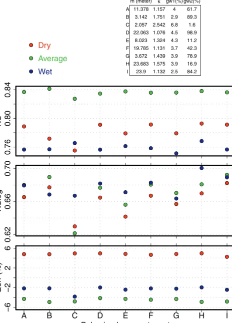
Fig.8.Selectedgroupofbehavioralparametersetsandtheircalibrationmetricsthatwereusedformodelsimulations.Anine behavioralparametersetscomprisedof(m(m),k,gw1(%),andgw2(%))wereshownintable(upperright).

Toaddresstheequifinalityconcept,whichstatesthattheremaybemanymodelsofacatchment thatacceptablyreproduceobservations,weselectedagroupofbehavioralparametersetsfromthe MonteCarlosimulations(Fig.7)thathadapercenterror(Qerr)of−5.0%≤Qerr≤5.0%,aNash–Sutcliffe efficiencyondailyflows(NS≥0.75),andaNash–Sutcliffeefficiencyonlogdailyflows(NSlog≥0.60). Ninebehavioralparametersetswereidentifiedthatsatisfiedallthethreementionedconditionsover thethreedifferentwateryearconditions(dry,averageandwet).Fig.8givesaplotofthenine behav-ioralparameterssetsselectedwithmodelperformancemetrics.InFig.8,welistattheupperright cornertheninebehavioralparameterswithvaluesofm(m),k,gw1(%),andgw2(%).Wegivethe modelperformancemetricscorrespondingtothedifferentwateryears(dry,average,andwet)for

0

100

200

300

400

0

100

200

300

400

Simulated (mm)

Observed (mm)

Fig.9.ScatterplotofmonthlyobservedandsimulatedrunoffinmmfortheMadRivernearMoretownwatershed(USGSgauge #04288000)inverificationofRHESSysduring1955to2010wateryears.RHESSysparametersusedtodrivemodelsimulations runoffresultswere:m=2.057(m),k=2.542,gw1=6.8(%),andgw2=1.6(%).

eachbehavioralparameterssetinred,green,andbluecolorsrespectively.Themodelperformance metricsshowninFig.8aretheNash–Sutcliffeefficiency(NS)fordailysimulatedandobservedrunoff, theNash–Sutcliffeefficiency(NSlog)fordailysimulatedandobservedrunoffinlog-scale,andthe per-centerror(Qerr)betweendailysimulatedandobservedrunoff.Wenotethattheaveragewateryear modelsolutionscapturemostofthevarianceobservedcomparedwithdryandwetyearsmodel solu-tions(NSaverage≈0.84).Wetwateryearmodelsolutionstotalannualflowerrorestimatesachieveda

closematchwithobservedrunoffvalues(QerrWet≈0%).

Fig.9showsmonthlyobservedandsimulatedrunoffforthestudywatershedasverificationof RHESSysmodelperformanceduring1955–2010wateryears.AsseeninFig.9,modelperformance isrobust.Theverificationperiodusedwasfromwateryear1955towateryear2010.Ingeneral,all theselectedbehavioralparametersetsareabletoexplainmorethan60%ofthevariance seenin observeddailyrunoff,andunderestimateobservedrunoffbyabout4%.Modelresultsgeneratedfrom eachoftheninebehavioralparametersetsshowthatpatternsandtrendsofsimulatedrunoffwere consistent.

Simulatedrunoffresultswithm=23.9(m),k=1.132,gw1=2.5(%),andgw2=84.2(%)parameterset (i.e.,groupIinFig.8)areabletoexplainabout79%ofthevarianceseeninobserveddailyrunoffduring thecalibrationdryyear,about84%ofthevarianceseeninobserveddailyrunoffduringthecalibration averageyear,andabout79%ofthevarianceseeninobserveddailyrunoffduringthecalibrationwet

0 5 10 15 20 25

mm/da

y

Cumulativ

e (mm)

mm/da

y

Cumulativ

e (mm)

Oct Dec Feb Apr Jun Aug

mm/da

y

Oct Dec Feb Apr Jun Aug

Cumulativ

e (mm)

Fig.10.Dailysimulatedversusobservedrunoff(mm)fortheMadRivernearMoretownwatershedincalibrationofRHESSys. Wet[row(a)],average[row(b)]anddry[row(c)]wateryieldyearresultsareshown.Rightpanelsgivecumulativerunoff (observedandsimulated),evapotranspirationandstoragesimulatedwithobservedprecipitationduringcorrespondingyearto theleft.

year(Fig.10).Dryyearwateryield(panela),averageyearwateryield(panelb)andawetyearwater yield(panelc)areshowninFig.10.Wealsopresentcumulativesimulatedrunoff,evapotranspiration andstorage(offsettobezeroatthestart)aswellasobservedprecipitationandrunoff.Themodel capturesmostofthevariabilityseenindailyrunoffduringspringbuttoalesserdegreeduringsummer time.ThisisshownwiththeNash–Sutcliffeefficiencyoflog-transformeddailyrunoffvaluesof0.79 (panela),0.84(panelb),and0.76(panelc).

Table3

AnnualprecipitationattheMadRiverwatershedduring1951–2005wateryearsMannKendalltrendanalysis.isthearithmetic meaninmeters,isunbiasedstandarddeviationinmeters,CViscoefficientofvariation(/),iscorrelationbetweengridded data(Maureretal.,2002)andtheCMIP5ensemble,(tau)isKendall’staucorrelationcoefficient,p-valueis2sided-test,Trend isHighlySignificantwhen(p≤0.001)andSignificantwhen(p≤0.05).

Datasource/climatemodelID CV (tau) p-Value Trend

Maureretal. 1.209 0.192 0.159 – 0.3859 0.00003 Highlysignificant

ACCESS1-0 1.192 0.104 0.087 0.011 0.0128 0.89603 Notrend BCC-CSM1-1 1.189 0.108 0.091 0.077 0.0492 0.60119 Notrend BNU-ESM 1.199 0.113 0.095 0.318 0.2162 0.02018 Significant CanESM2 1.193 0.117 0.098 0.064 0.0626 0.50421 Notrend CCSM4 1.200 0.105 0.088 −0.077 0.0303 0.74941 Notrend CESM1-BGC 1.200 0.094 0.079 0.208 0.2040 0.02835 Significant CNRM-CM5 1.193 0.111 0.093 0.180 0.1960 0.03527 Significant CSIRO-Mk3-6-0 1.203 0.133 0.111 0.126 −0.0020 0.98842 Notrend GFDL-CM3 1.200 0.101 0.084 −0.205 0.0626 0.50421 Notrend GFDL-ESM2G 1.197 0.099 0.082 0.025 0.1300 0.16337 Notrend GFDL-ESM2M 1.198 0.117 0.097 0.158 0.1582 0.08937 Notrend INM-CM4 1.189 0.107 0.090 −0.063 0.1205 0.19629 Notrend IPSL-CM5A-LR 1.201 0.111 0.092 0.168 0.2485 0.00755 Significant IPSL-CM5A-MR 1.197 0.093 0.078 0.033 0.1098 0.23958 Notrend MIROC-ESM 1.194 0.093 0.078 −0.062 0.0909 0.33066 Notrend MIROC-ESM-CHEM 1.202 0.108 0.090 −0.161 0.0653 0.48586 Notrend MIROC5 1.184 0.123 0.104 0.008 −0.0397 0.67372 Notrend MPI-ESM-LR 1.196 0.112 0.094 0.075 0.0007 1.00000 Notrend MPI-ESM-MR 1.184 0.105 0.089 0.027 −0.0478 0.61134 Notrend MRI-CGCM3 1.198 0.100 0.083 0.124 0.1407 0.13105 Notrend NorESM1-M 1.195 0.082 0.068 0.079 0.2094 0.02442 Significant

3.2. Globalclimatemodelshistoricaltrendsandvariabilities

Ananalysisoftwenty-onehindcastCMIP5modeloutputdatasetswasperformedtoassessthe variabilityandtrendofeachdatasetcomparedtotheobservedhistoricaldataofMaureretal.(2002). Theprecipitationcoefficientofvariation(CV)andtrend(representedbyKendall’stau)arepresentedin

Table3.AsnotedbythediscrepancyinKendall’staucomparedtotheobservations,noneoftheCMIP5

datasetsadequatelyreproducestheobservedprecipitationtrend.OnlyfiveCMIP5modeloutputsshow astatisticallysignificantincreasingtrend(whichisfarlowerinmagnitudethantheobserved),and thosefivearechosenasasubsetonthatbasisforfurtheranalysisinthiswork.Moreover,comparison oftheprecipitationcoefficientofvariationoftheCMIP5andobserveddatasetsshowsthatnoneof theCMIP5modelsadequatelyreproducestheobservedvariability,whichlimitstheabilitytosimulate extremeevents.

Thefailureofthehindcastclimatedatatoreproducetheobservedtrendcallsintoquestionthe validityoftheprecipitationforecastdataasanadequatedriverofhydrologymodelsforthesimulation ofclimatechangeimpacts.Therefore,foranalternatescenario,wesuperimposedtheobservedtrend inthehistoricalprecipitation(+7mm/year)ontherelativelyflatCMIP5precipitationdataforuseasa driverofthehydrologymodelpresentedinthiswork.Thisapproachassumesthattheobservedtrend willcontinueunchangedinthefuture,andallowsassessmentofthepossiblehydrologicflowregime resultingfromincreasingprecipitation.Hydrologymodelsimulationresultsusingbothalteredand unalteredprecipitationinputtimeseriesarecomparedtoemphasizetheimportanceoftrendinthe CMIP5data.TheCMIP5productsreproduceobservedtemperaturetrends,whichwereleftunaltered. TheRHESSysmodelwasruninaretrospectivemodetoproducehistoricalrunoffsimulationsusing thehistorical CMIP5climatedata(1955–2005)asaclimatedriver.Theannualrunoffsimulations (retrospectiveclimatedatafromfiveclimatemodelsundertwoscenarios)showadifferenttrendand variabilitywhencomparedtohistoricalobservedrunoffdata(Fig.11).Fig.11showsbothtimeseriesas wellasdistributions(representedbyboxplots)toillustratethesedifferencesintrendandvariability. Meanannualrunofffromallclimatemodelswasclosetoobservedrunoff.However,interquartile annualrunoffrangeofallclimatemodelstestedwaslessthanobservedannualrunoff.Notsurprisingly,

1960 1980 2000 400 600 800 1000 Runoff (mm) OBSERVED BNU−ESM CESM1−BGC CNRM−CM5 IPSL−CM5A−LR NorESM1−M

OBSERVED Trend (loess−R default)

GCMs Average Trend (loess−R default)

400

600

800

1000

Runoff (mm)

OBSERVED BNU−ESM CESM1−BGC CNRM−CM5 IPSL−CM5A−LR NorESM1−M

Fig.11. AnnualobservedandretrospectivesimulatedrunoffattheMadRivernearMoretownwatershed(USGSgauge# 04288000).Dataarerunoffforthewateryears1955–2005.RunoffsimulationswereobtainedbyhindcastingtheRHESSys modelwithfiveclimatemodelsfromtheCMIP5ensemblesdataandtheninebehavioralsetsdiscussed.Trendsshownwere obtainedusingthelocalpolynomialregressionfitting(loess)functionwithdefaultparametersinRsoftwarepackage.

climatemodel-drivenrunoffsimulationshaveclearlyunderestimatedthehistoricalobservedrunoff trendbecauseofthelackoftrendinCMIP5precipitationdata.Differencesintrendsarevisualized usinglocalpolynomialregressionfittingfunction(loess)evaluatedfromthedefaultparametersinthe

Rsoftwarepackage(Clevelandetal.,1992;RDevelopmentCoreTeam,2014).Theseresults(Fig.11) showthatclimatemodeldatahavenotsucceededinproducinghistoricalobservedrunofftrendsand variabilitieswhenappliedonaregionalscalestudy.

3.3. Modelprediction

RunoffsimulationsshowninFigs.12–15wereobtainedbydrivingtheRHESSysmodelwith ensem-blesfrom:(i)thesubsetoffiveCMIP5climatemodelsthatshowsignificanttrendinprecipitation,and (ii)thefiveclimatemodelsfromtheCMIP5withthesuperimposedtrendasdescribedearlier(Section

2.3).Inbothofthetwosetsofensembles,weconsideredthetwoclimatescenarios(RCP4.5andRCP 8.5).ThefiveclimatemodelsshowninFigs.12–15are,a:BNU—ESM;b:CESM1—BGC;c:CNRM—CM5; d:IPSL—CM5A—LR;ande:NorESM1—M.Anoticeableincreaseinnumberoffloodeddayshasbeen observed.Inaddition,arepeatedpatternoffloodoccurrencesisevidentacrossalltheclimatemodel studieswithvariationsinduration.

Fig.12showskerneldensityestimatesofthedistributionofmaximumflooddurationdaysatour studywatershed,usingthefloodthresholdof15mm/day(2,175cfs).The1964–2013lineinFig.12

isthekerneldensityestimateofflooddurationdaysusingthefloodthresholdof15mm/dayduring 1964–2013wateryears.Future(i.e.,2016–2099wateryears)kerneldensityestimatesoffloodduration dayswereobtainedbydrivingtheRHESSysmodelwithfiveclimatemodelsfromtheCMIP5ensembles (subscript1)aswellasthesuperimposedtrendensembles(subscript2)consideringthetwoscenarios (i.e.,RCP4.5andRCP8.5)andtheninebehavioralsetsdiscussed.Theestimatedbandwidththatthe

SheatherandJones(1991)methodgivesforthevariousdistributionsshowninFig.12varybetween

0.1and1.7days.Forconsistency,sothatmodedifferencesarenotduetobandwidthdifferences,Fig.12

wasplottedusingtheaveragebandwidthof0.8days.Tochecksensitivitytobandwidth,wealsoplotted densityestimateswithrangeofbandwidthsspanning0.1–1.7daysandobtainedfigures(notshown)

0

5

10

15

20

0.00

0.05

0.10

0.15

0.20

0.25

Flood Duration (Days)

Density

0

5

10

15

20

Flood Duration (Days)

Fig.12. KerneldensityestimateoftheflooddurationindaysattheMadRivernearMoretownwatershed(USGSgauge# 04288000)observedandprojectedfrommodelsimulations.Theflooddurationindaysarethenumberofdayswhenrunoff equalsorexceedsarunoffmagnitudeof15mm/day(i.e.,dailydischargeof2,175cfs).Kerneldensitylinelabeled(b-1)refers totheCESM1—BGCclimatemodelensemblesflooddurationscenario,whilekerneldensitylinelabeled(c-2)referstothe CNRM—CM5climatemodelwithsuperimposedtrendensemblesflooddurationscenario.

1960 1980 2000 2020 2040 2060 2080 2100 5 10 15 20 25 30 7QMAX (mm/d a y) (1) ● ● ● ● ● ● ● ● ● ● ● ● ● ● ● ● ● ● ● ● ● ● ●●●●●●●●●●●●●●●● ●●●●●●●●●●●●●●●● ● ● ● ● ● ● ● ● ● ● ● ● ● ● ● ● ● ● ● ● ● ● ● ● ● ● ● ● ● ● ● ● ● ● ●● ● ● ● ● ● ● ● ● ● ● ● ● ● ● ● ● ● ● ● ● ● ● ● ● ● ● ● ● ● ● ● ● ● ● ● ● ● ● ● ● ● ● ● ● ● ● ● ● ● ● ● ● ● ● ● ● ● ● ● ● ● ● ● ● ● ● ● ● ● ● ● ● ● ● ● ● ● ● ● ●

HISTORICAL CESM1−BGC IPSL−CM5A−LR

(1) 5 10 15 20 25 30 1960 1980 2000 2020 2040 2060 2080 2100 5 10 15 20 25 30 7QMAX (mm/d a y) (2) ● ● ● ● ● ● ● ● ● ● ● ● ● ● ● ● ● ● ● ● ● ● ● ● ● ● ● ● ● ● ● ● ● ● ● ● ● ● ● ● ● ● ● ● ● ● ● ● ● ● ● ● ● ● ●●_●●●●_●●●●_●●●●●●●●●●●●●●●●●●●● ● ● ● ● ● ● ● ● ● ● ● ● ● ● ● ● ● ● ● ● ● ● ●●●●●●●●●●●●●●●●●●●● ● ● ● ● ● ● ● ● ● ● ● ● ● ● ● ● ● ● ● ● ● ● ● ● ● ● ● ● ● ● ● ● ● ● ● ● ● ● ● ● ● ● ● ● ● ● ● ● ● ● ● ● ● ● ● ● ● ● ● ● ● ● ● ● ● ● ● ● ● ● ● ● 5 10 15 20 25 30 BNU−ESM CNRM−CM5 NorESM1−M (2)

Fig.13.Seven-daymaximumflowattheMadRivernearMoretownwatershed(USGSgauge#04288000).Rightpanelsgive boxplotsofseven-daymaximum(7QMAX)dataforthehistorical(1955–2013)andsimulated(2016–2099)wateryearrunoffs. Panelsnumberedwith1refertotheCMIP5ensembles,whilepanelsnumberedwith2refertotheCMIP5withsuperimposed trendensembles.

1960 1980 2000 2020 2040 2060 2080 2100 10 20 30 40 50 BFI (%) (1) ● ● ● ● ● ● ● ● ● ● ● ● ● ● ● ● ● ● ● ● ● ● ●● ● ● ● ● ● ● ● ● ● ● ● ● ● ● ● ● ● ● ● ● ●●●●●●●● ● ● ● ● ● ● ● ● ● ● ● ● ● ● ● ● ● ● ● ● ● ● ● ● ● ● ● ● ● ● ● ● ● ● ● ● ●●●●●●●●●●●●●●●● ● ● ● ● ● ● ● ● ● ● ● ● ● ● 10 20 30 40 50 (1)

HISTORICAL CESM1−BGC IPSL−CM5A−LR

1960 1980 2000 2020 2040 2060 2080 2100 10 20 30 40 50 BFI (%) (2) ● ● ● ● ● ● ● ● ● ● ● ● ● ● ● ● ● ● ● ● ● ● ● ● ● ● ● ● _●●●●●●_●● ● ● ● ● ● ● ●_●●●●●●_●●●●●●●●●●●●●_●● ●●●●●● ● ● ● ● ● ● ● ● ● ● ● ● ● ● ● ● ● ● ● ● ● ● ● ● ● ● ● ● ● ● ● ● 10 20 30 40 50 BNU−ESM CNRM−CM5 NorESM1−M (2)

Fig.14. Baseflowindex(BFI)attheMadRivernearMoretownwatershed(USGSgauge#04288000).Rightpanelsgiveboxplots ofbaseflowindexdataforthehistorical(1955–2013)andsimulated(2016–2099)wateryearrunoffs.Panelnumberfollows namingconventionusedearlierinFig.13.

thatwereverysimilartoFig.12,withmodesatthesamelocations.Wethereforeconcludedthat interpretationswerenotsensitivetotheselectionofbandwidthintherangeresultingfromdifferent datalengths.Wealsolookedattimeseriesplotsfortheabovementioneddistributions(notshown) andfoundthatroughlyevery25yearsthereisapeakinnumberoffloodeddays.Ourresults,using

Historical Contingency Constancy 0 0.2 0.4 Predictability RCP 4.5 RCP 8.5 (a−1) RCP 4.5 RCP 8.5 (b−1) RCP 4.5 RCP 8.5 (c−1) RCP 4.5 RCP 8.5 (d−1) RCP 4.5 RCP 8.5 (e−1) Historical 0 0.2 0 .4 Predictability RCP 4.5 RCP 8.5 (a−2) RCP 4.5 RCP 8.5 (b−2) RCP 4.5 RCP 8.5 (c−2) RCP 4.5 RCP 8.5 (d−2) RCP 4.5 RCP 8.5 (e−2)

Fig.15.Colwellindex,Predictability(P),Constancy(C),andContingency(M)ofrunoffattheMadRivernearMoretown water-shed(USGSgauge#04288000).Dataaredailyrunoffforthewateryears1955–2013(historical)andsimulatedrunoffforthe wateryears2016–2099(future).PanelnumberfollowsnamingconventionusedearlierinFig.12.

asuperimposedincreasingprecipitationtrendreflectedinthehistoricalrecord,predictfourmore floodeddaysinthecomingcenturyrelativetothehindcastperiod.

UsingtheunalteredCMIP5dataasinput(RCP4.5andRCP8.5),modelresultsdonotshowa sig-nificantchangeinthehighestflows(7QMAX),despitefutureprojectionsofincreasedprecipitation intheregion(Fig.13,part1).Thismayrepresenttheroleofsoilmoistureorsnowpackdynamics. However,asignificantchangeisshownforthecaseofsuperimposedprecipitationtrendensembles. Resultssuggestthatthemedianofthesevenmaximumrunoff7QMAXwillchangeby30%inthefuture (Fig.13,part2).

Wealsoassessedclimate-inducedchangesinlowflowdisturbances.Ourresultssuggestthatboth variablesthatquantifylowflowdisturbances(BFIand7QMIN)showedasignificantincreaseinthe future.Wenotedanincrease ofaboutthree ordersofmagnitudeinthebaseflow indexvariable (Fig.14).Thisincreaseinlowflowregimeisevidentthroughtheuseofalltheclimatemodelsstudied. InFig.14,weshowboxplotsofhistoricandfuturebaseflowindicestoillustratethedegreeofincreased change.Thetimingassociatedwiththisincreaseisduringsummer(June21th_{toSeptember20}th_).The 7-dayminimum(7QMIN)variablebehaviorhasnotbeenshownsinceitconveysthesameinformation. ThisfindingisconsistentwiththerecentobservationofHodgkinsandDudley(2011)indicatingthat thelatterhalfofthetwentiethcenturyhaswitnessedanincreaseinsummerflowsinNewEngland.

Modelpredictionsdidnotindicateasignificantchangeinflowreversaldaysunderfutureclimate scenarios.Somemodelssuggestdecreasednumberofreversaldayswhileotherssuggestincreased numberofreversaldays.Wethinkthatthequalityofourpredictionresultsdidnotsucceedtomanifest aclearflowvariabilitysignal(inputclimatedataandmodelefficiencytocapturestreamflowvariance). Theseresultsconveyalimitationofourmodelingeffortstoassessstreambanksdamagesanticipated withclimatechange.

Model outputshows a 60% increase in theColwell indexrunoff predictability metric for the 2015–2099wateryearsperiodamongallmodelstested.Bothconstancyandcontingencyareshown asbarplotsinFig.15toillustratetheColwellindexcomponents.Wenotethatthecontingencyis min-imalwhichmeansthattheprobabilityofoccurrenceofeachflowstateisindependentofthemonth (homogenousmonthlyflowtimeseries).Weinferthatexpectedrunoffatthisstudywatershedwould haveadifferentmonthlypatternordistributioncomparedtohistoricaldataobserved.Monthlyrunoff patternchangewillaffectthequalityofthewatershedhabitatandcauseecologicalconsequenceson fisheriespopulations.

4. Discussion

TheCMIP5dataproducts(Tayloretal.,2011;Meehletal.,2014)arewidelyusedforregionalclimate changeimpactsanalysis.However,forourstudyareainnorthwesternNewEngland,onlyfiveclimate modelsshowedstatisticallysignificanttrendsinprecipitationinhindcast,butthemagnitudeofthese trendsarenotadequatelyrepresentativeofthoseseeninobservedannualprecipitation.Toaddress thisdiscrepancyinhistoricalprecipitationtrend,weextrapolatedtheobservedhistoricalprecipitation trendtoprovideanupperenvelopeofpredictionsoffuturehydrologicalimpactsassociatedwith climatechange.Theuseofanextrapolatedobservedtrendcannotcaptureregionalclimatepatterns inducedbylarge-scalechangesincirculationordecadal-scaleclimaticoscillations(suchastheNorth AtlanticOscillationorArcticOscillation),andthereforefuturedatasetswithextrapolatedtrendsmust beusedwithgreatcaution.However,itisclearfromthisanalysisthatCMIP5productsareinsufficient forregionalhydrologicanalysisinVermontbecausethetrendandvariabilityareunderrepresented. Theuseofanyofthetwenty-oneCMIP5modelsavailablewouldleadtorunoffsimulationsthatshow nochangeinhighflows.Suchaconclusioncoulderroneouslybeusedasabasisfora“donothing” approachbypolicymakersforadaptationtoclimatechange,wheninfactincreasingprecipitation cancausenumerousadversehydrologicimpacts,suchasanincreasedfloodriskandexacerbated nonpointsourcepollution.WedemonstratethelargedifferenceinflowregimewhenusingtheCMIP5 datawithasuperimposedtrendcomparedtoonlyunalteredCMIP5datausingthebestfivedatasets. Thenear-term(4–5decades)predictedflowsusingthesuperimposedtrenddatasetmaybeusefulfor designandplanningasabasicscenarioforadaptationtoclimatechangeinhighgradientwatersheds innorthwesternNewEngland.

Inadditiontothelackofareproducedtrendinprecipitation,recentworkhasdescribedthefailure oftheCMIP5datatocaptureincreasedintensity,durationandfrequencyofprecipitationextremes, whichisconsistentwithourfindingofinadequaterepresentationofvariabilityintheprecipitation processinVermont(Wuebblesetal.,2013).Therefore,thechangingprobabilityoftheuppermost quantilesisnotwellrepresentedusingourapproach.Themean,variability,andskewnessoffloware allexpectedtochangewithclimatechange,butthepresentedapproachonlyallowsforchangesin thefirsttwomoments.

OurapproachtoprojectingfutureflowregimeinnorthwesternNewEnglandhasnotincorporated thenonlinearinterconnectivityandfeedbacksbetweenclimatevariablesandvegetationcover. More-over,thehydrologicalmodelusedinourapproachdidnotincludeincorporationofimpactsofincreased CO2concentrationsonstomatalphysiologyofforests,changesinspeciescompositionordistribution, andtheresponseofleafareaindextoclimatechange.Vegetationfeedbackscouldactinvariousways toexacerbateoroffsetourprojectedchangesinstreamflow.CO2fertilizationwouldbeexpectedto reducestomatalconductanceandincreasewateruseefficiency,therebydecreasing evapotranspira-tion(ET)andincreasingstreamflowduringthegrowingseason,asdiscussedbyCampbelletal.(2011), thoughtheirmodelprojectionsofstreamflowincorporatingCO2fertilizationresultedinincreasing trendsinfutureETattheHubbardBrookExperimentalForestinnearbyNewHampshire.Warmer con-ditionsinthefuturemightalternativelylengthenthegrowingseasonforforestsintheregion(Betts,

2011;Richardsonetal.,2012;Whiteetal.,2014).Afuturetrendoflengthenedleaf-onperiodwould

resultindaystoweeksofextendedET,offsettingsomeoftheincreasedfutureprecipitationand mit-igatingagainstincreasingbaseflow.Amorecomplexandyetunexaminedimpactofclimatechange onvegetation-waterrelationswouldbeassociatedwithchangesinforesthealthandspecies com-positionthatwoulddrivechangesinETdemandsandresultingstreamflow.Decliningforesthealth andassociatedreductionsinETcouldleadtoincreasesinbaseflowgreaterthanthelevelsweproject here.Thestepchangesinthebaseflowindexprojectedinoursimulationsaredrivenbytheprojected lineartrendinincreasingprecipitationanddonotincludethesemorecomplexvegetation-climate interactionsthatmayalterfuturestreamflows.Ingeneral,ourabilitytoprojectflowregimeshould beassessedconsideringthisuncertainty.

Ourresultssuggestarepeatedpatternoffloodoccurrenceswithincreasedfrequency.Somestudies havesuggestedthatthisrepeatedmodeoffloodoccurrencesinourstudyregioniscorrelatedwith climateindexoccurrencesattheregionsuchastheNorthAtlanticOscillation(NAO)(Huntingtonetal.,

2004;GriffithsandBradley,2007;Brownetal.,2010).Thisrepeatedphenomenonoffloodoccurrences

maylikelybeattributedtohemisphericscaleandpotentiallyregionalscaleatmosphericcirculation patterns,howevertheexpectedwarmedclimatemayinfluencetheseatmosphericcirculationindices themselves,hencethereisgreatuncertaintyinfuturefloodsignals(Visbecketal.,2001).

Flowvariabilityisanimportantaspectofthestreamflowregime.Thereisanongoingdiscussion withintheLakeChamplainmanagementcommunityaswellasthestateandfederalenvironmental protectionagenciesconcerningtheLakeChamplainsedimentandnutrientloads(StagerandThill, 2010).Theanticipatedfutureincreasedmaximumflowswilllikelygreatlyexceedcurrentsediment andnutrientloadingtotheLake,continuingatrendofdecliningwaterqualityinLakeChamplain(Lake

ChamplainBasinProgram,2012).

TheMadRiverwatershedphysicalhabitatisforBrownandBrooktrout,Longnosedace,andSlimy sculpinbutinsomereaches,thewaterqualitylimitsfishpopulations.Fishpopulationsinhabiting Vermontstreamsandriversingeneralhaveadaptedtoflooding(Kirn,2011).However,giventhe expectedchangesinclimate(temperatureincrease)andtheassociatedstreamflowtemporalpatterns change(Colwell’spredictabilityincrease)thefutureadaptationshouldbeconsidered.Theanticipated hydrologicalimpactspresentedhereinmayassistongoingresearchthatinvestigatestheseecological responsestoclimatechangeinLakeChamplainecosystem(Warrenetal.,2012).

ThepresentedworkcriticallyassessestheabilityoftheCMIP5ensembletoadequatelycapture thedynamicsofclimateconditionsoverthehistoricperiodatourstudyregionforuseinhydrologic impactanalysis.Ourfuturesimulationresultshighlightthesubstantialdifferencesbetweentheuseof CMIP5andtrend-extrapolatedobservations,underscoringtheneedtobeverycautiouswhenapplying climatemodelproductsforregionalanalysis.However,thepredictionresultspresentedinthiswork shouldbeviewedasbestestimatesofwhatisavailable.Understandingchangesinstreamflowregime

requiresabetterknowledgeofclimatedata,runoffmodelsparameters,andrepresentationofphysical processes.Inordertoobtainthatknowledge,extensivefieldeffortsintendedtoexaminehydrological modelsensitivitiestoclimateandhydrologicalmodelparametersarerequired.

5. Conclusions

UsingtheCMIP5climatedataforregionalhydrologicanalysistomakerunoffprojectionstoinform planningandpolicywouldbefundamentallyproblematiciftheclimatemodelsarenotadequately validatedforaregionofinterest.ManyoftheforcingCMIP5datafailtocaptureboththetrends andvariabilityobservedinprecipitationwhenruninhindcast.Thisstudyhasshownthepotential differencesinsimulatedflowmetricsiftheCMIP5dataisapplieduncritically,andshowsthatCMIP5 failstocapturetrendstowardincreasedprecipitationinVermont.

Nevertheless,whendrivenbytheCMIP5datacorrectedfortrend,thehydrologicalmodelused inthisstudypredictsanincreaseinhighflows,lowflows,andadecreaseintheuncertaintyseenin temporalpatternsofrunoffduringthe21stcenturyforcentralVermont.Thetrend-corrected sim-ulationshowsanincreaseof30%inseven-daymaximumflow,fourdaysincreaseinfloodeddays, threeordersofmagnitudeincreaseinbaseflowindex,anda60%increaseinrunoffpredictability.The above-mentionedresultsreflecttheneedtoadapttoincreasedfloodrisk,updatedfloodplain man-agement,exacerbatednonpointpollutionloadingtoLakeChamplain,andotherproblemsassociated withhigherfutureflows.

Acknowledgements

ThisworkwassupportedbytheVermontExperimental Programfor StimulatingCompetitive Research(EPSCoR)AwardnumberNSFEPSGrant#1101 1 .TheauthorsacknowledgetheVermont AdvancedComputingCorewhichissupportedbyNASA(NNX06AC88G),attheUniversityof Ver-montforprovidingHighPerformanceComputingresourcesthathavecontributedtotheresearch resultsreportedwithinthispaper.WeacknowledgetheWorldClimateResearchProgramme’s Work-ingGrouponCoupledModelling,whichisresponsibleforCMIP,andwethanktheclimatemodeling groups(listedinTableA-1ofthispaper)forproducingandmakingavailabletheirmodeloutput.For CMIP,theU.S.DepartmentofEnergy’sProgramforClimateModelDiagnosisandIntercomparison providescoordinatingsupportandleddevelopmentofsoftwareinfrastructureinpartnershipwith theGlobalOrganizationforEarthSystemSciencePortals.Theauthorsareindebtedtotwoanonymous reviewersfortheirconstructiveandthoroughreviews.

3 7

AppendixA.

TheWorldClimateResearchProgramme(WCRP)developedglobalclimateprojectionsthroughits CoupledModelIntercomparisonProject5(CMIP5).Weexaminedtwenty-oneprojectionensembles ofCMIP5downscaledbythedailybias-correctionandconstructedanalogs(BCCA)statistical down-scalingtechniqueavailableat(http://gdo-dcp.ucllnl.org/downscaledcmipprojections/)accessedon 27May2014andlistedinTableA1.MannKendalltrendanalysis(HelselandHirsch,2002)wasused toexaminewhetheranytrendsinprecipitationdatawerestatisticallysignificant.Table3givestrend analysisresultsforthehistoricobservedannualprecipitation(Maureretal.,2002)aswellastheCMIP5 projectionensembleshindcastdataoverourstudywatershed.Thistableincludesthemeanannual precipitation,,theannualstandarddeviation,,thecoefficientofvariation,CV,thecrosscorrelation betweenclimatemodelensemblesandobservedprecipitation,,theKendall’staucorrelation coeffi-cient,,aswellasthep-valueassociatedwiththeMannKendalltest.Table3showsthattheyarefive climatemodelensembleswithsignificantincreasingtrend(p<0.05)inannualprecipitation.Namely, thesefiveclimatemodelingcentersare:theCollegeofGlobalChangeandEarthSystemScience,Beijing NormalUniversity(BNU—ESM);theCommunityEarthSystemModelContributors(CESM1—BGC);the CentreNationaldeRecherchesMétéorologiques/CentreEuropéendeRechercheetFormationAvancée enCalculScientifique(CNRM—CM5);theInstitutPierre-SimonLaplace(IPSL—CM5A—LR);andthe Nor-wegianClimateCentre(NorESM1—M).Amongthetwenty-oneprojectionensemblesanalyzed,these

TableA1

CoupledModelIntercomparisonProject(CMIP5)groupsstudied.

No. Modelingcenter(orgroup) InstituteID Modelname

1 CommonwealthScientificandIndustrialResearch OrganizationandBureauofMeteorology,Australia

CSIRO-BOM ACCESS1-0

2 BeijingClimateCenter,ChinaMeteorological Administration

BCC BCC-CSM1-1

3 CollegeofGlobalChangeandEarthSystemScience, BeijingNormalUniversity

GCESS BNU-ESM

4 CanadianCentreforClimateModellingandAnalysis CCCMA CanESM2

5 NationalCenterforAtmosphericResearch NCAR CCSM4

6 CommunityEarthSystemModelContributors NSF-DOE-NCAR CESM1-BGC

7 CentreNationaldeRecherches

Météorologiques/CentreEuropéendeRechercheet FormationAvancéeenCalculScientifique

CNRM-CERFACES CNRM-CM5

8 CommonwealthScientificandIndustrialResearch Organization,QueenslandClimateChangeCentreof Excellence CSIRO-QCCCE CSIRO-Mk3.6.0 9 NOAAGeophysical FluidDynamics Laboratory NOAAGDFL GFDL-CM3 10 GFDL-ESM2G 11 GFDL-ESM2M

12 InstituteforNumericalMathematics INM INM-CM4

13 InstitutPierre-Simon Laplace

IPSL IPSL-CM5A-LR

14 IPSL-CM5A-MR

15 JapanAgencyforMarine-EarthScienceand Technology,AtmosphereandOceanResearch Institute(TheUniversityofTokyo),and NationalInstituteforEnvironmentalStudies

MIROC MIROC-ESM

16 MIROC-ESM-CHEM

17 AtmosphereandOceanResearchInstitute(The UniversityofTokyo),NationalInstitutefor EnvironmentalStudies,andJapanAgencyfor Marine-EarthScienceandTechnology

MIROC MIROC5

18 Max-Planck-InstitutfürMeteorologie(Max PlanckInstituteforMeteorology)

MPI-M MPI-ESM-LR

19 MPI-ESM-MR

20 MeteorologicalResearchInstitute MRI MRI-CGCM3

21 NorwegianClimateCentre NCC NorESM1-M

fivemodelsshowedarelativelyclosecorrelationwithobservedprecipitationdata.Weadoptedusing thesefiveclimatemodelensemblesforthiswork.

AppendixB.

FlowpredictabilityvariablesusedinthispaperareColwell’sindices(Colwell,1974).Colwell’sindices arepredictability(P),constancy(C)andcontingency(M).Constancy(C)andcontingency(M)are quan-tifiedbasedonentropymeasuresofuncertaintyfromShannon’sinformationtheoryeitheracrossall months(C),orcontingentuponaspecificmonth(M)(Jelínek,1968).Predictability(P)hastwoseparable components:constancy(C)andcontingency(M).Predictabilitycombinesconstancyandcontingency throughP=C+M.CalculationofColwell’sindicesP,CandMrequiresthatvaluesbebinnedintodiscrete groups.

Predictability(P)istheconverseofuncertainty,itisreasonablethentobasemeasuresof predictabil-ityanditscomponents,constancy(C)andcontingency(M),onthemathematicsofinformationtheory

(Colwell,1974).FollowingColwell,forafrequencymatrix(contingencytable)withtcolumns(times

phenomenonwasinstateiattimej.Definethecolumntotals(Xj),rowtotals(Yi),andthegrandtotal (Z)as: Xj= s

Thentheuncertaintywithrespecttotimeis H(_X)₌₋ t

theuncertaintywithrespecttostateis H(Y)=− s

andtheuncertaintywithrespecttotheinteractionoftimeandstateis H(XY)=−

Thepredictabilityofaperiodicphenomenonismaximalwhenthereiscompletecertaintywith regardtostate(row)oncethepointintime(column)isspecified.Intermsofinformationtheory,the conditionaluncertaintywithregardtostate,withtimegiven,isdefinedas(Jelínek,1968)

HX(Y)=H(XY)−H(X).

Whenpredictabilityisatitsminimum,allstatesareequiprobableforalltimes.InthiscaseH(X)=log t,andH(XY)=logst,sothatHX(Y)=logs.Toobtainmeasureofpredictability(P)withtherange(0,1),

define

P=1−HX(Y) logs =1−

H(XY)−H(X) logs .

Constancyismaximizedwhenallrowtotalsbutonearezero;itisminimizedwhenallrowtotals areequal.SinceH(Y)variesinpreciselytheoppositeway,anditsmaximumvalueislogs,ameasure ofconstancy(C)withrange(0,1)isgivenby

C=1−H(Y) logs.

Contingency representsthe degree to which time determines state, or thedegree to which theyare dependent oneach other. In information theory, contingency is measuredby a quan-tity called average mutual information (Jelínek, 1968). Colwell (1974) cites contingency as the average amount of information about the state of the phenomenon provided by time or

I(XY)=H(Y)−HX(Y)=H(Y)+H(X)−H(XY).

Colwell(1974)givesanadjustedmeasureofcontingency(M),withrange(0,1)as

References

Band,L.E.,Patterson,P.,Nemani,R.,Running,S.W.,1993.Forestecosystemprocessesatthewatershedscale:incorporating hillslopehydrology.Agric.ForestMeteorol.63,93–126,http://dx.doi.org/10.1016/0168-1923(93)90024-C.

Band,L.E.,Mackay,D.S.,Creed,I.F.,Semkin,R.,Jeffries,D.,1996.Ecosystemprocessesatthewatershedscale:sensitivityto potentialclimatechange.Limnol.Oceanogr.41,928–938,http://dx.doi.org/10.4319/lo.1996.41.5.0928.

Betts, A.K., 2011. Vermont climate change indicators. Weather Climate Soc. 3, 106–115, http://dx.doi.org/10.1175/ 2011WCAS1096.1.

Brekke,L.,Thrasher,B.L.,Maurer,E.,Pruitt,T.,2013.DownscaledCMIP3andCMIP5ClimateProjections:ReleaseofDownscaled CMIP5ClimateProjections,ComparisonwithPrecedingInformation,andSummaryofUserNeeds.U.S.Dept.oftheInterior Tech.Rep.,BOR,Denver.

Brown,P.J.,Bradley,R.S.,Keimig,F.T.,2010.ChangesinextremeclimateindicesforthenortheasternUnitedStates,1870–2005. J.Climate23,6555–6572,http://dx.doi.org/10.1175/2010jcli3363.1.

Campbell,J.L.,Driscoll,C.T.,Pourmokhtarian,A.,Hayhoe,K.,2011.Streamflowresponsestopastandprojectedfuturechanges inclimateattheHubbardBrookExperimentalForest,NewHampshire,UnitedStates.WaterResour.Res.47,W02514, http://dx.doi.org/10.1029/2010wr009438.

Chinnayakanahalli,K.J.,Hawkins,C.P.,Tarboton,D.G.,Hill,R.A.,2011.Naturalflowregime,temperatureandthe composi-tionandrichnessofinvertebrateassemblagesinstreamsofthewesternUnitedStates.FreshwaterBiol.56,1248–1265, http://dx.doi.org/10.1111/j.1365-2427.2010.02560.x.

Cleveland,W.S.,Grosse,E.,Shyu,W.M.,1992.Localregressionmodels.In:Chambers,J.M.,Hastie,T.J.(Eds.),StatisticalModels inS.Wadsworth&Brooks/Cole,PacificGrove,CA,p.608.

Colwell, R.K., 1974. Predictability, constancy, and contingency of periodic phenomena. Ecology 55, 1148–1153, http://dx.doi.org/10.2307/1940366.

Dingman,S.L.,2002.PhysicalHydrology,2nded.PrenticeHall,UpperSaddleRiver,NJ,646pp.

Dunne,T.,Leopold,L.B.,1978.WaterinEnvironmentalPlanning.W.H.FreemanandCompany,NewYork,818pp.

Gibson,C.A.,Meyer,J.L.,Poff,N.L., Hay,L.E.,Georgakakos,A.,2005. Flowregimealterationsunderchangingclimatein tworiverbasins:implicationsforfreshwaterecosystems.RiverRes.Appl.21,849–864,http://dx.doi.org/10.1002/rra. 855.

Gordon,N.D.,McMahon,T.A.,Finlayson,B.L.,Gippel,C.J.,Nathan,R.J.,2004.StreamHydrology:AnIntroductionforEcologists, 2nded.JohnWiley&Sons,Chichester,England,429pp.

GRASSDevelopmentCoreTeam,2012.GeographicResourcesAnalysisSupportSystem(GRASS)Software,Version6.4.2. Fon-dazioneMach–CentreforAlpineEcologyCEA,Trento,Italy,Availableat:http://grass.osgeo.org/

Griffiths,M.L.,Bradley,R.S.,2007.Variationsoftwentieth-centurytemperatureandprecipitationextremeindicatorsinthe northeastUnitedStates.J.Climate20,5401–5417,http://dx.doi.org/10.1175/2007jcli1594.1.

Hartley,S.,Dingman,S.L.,1993.Effectsofclimaticvariabilityonwinter-springrunoffinNewEnglandriverbasins.Phys.Geogr. 14,379–393.

Hauer, F.R., Baron, J.S., Campbell, D.H., Fausch, K.D., Hostetler, S.W., Leavesley, G.H., Leavitt, P.R., McKnight, D.M., Stanford, J.A., 1997. Assessmentof climatechange andfreshwater ecosystemsof theRockyMountains, USAand Canada.Hydrol.Process.11,903–924,http://dx.doi.org/10.1002/(sici)1099-1085(19970630)11:8<903::aid-hyp511>3.0.co; 2-7.

Hayhoe,K.,Wake,C.,Huntington,T.,Luo,L.,Schwartz,M.,Sheffield,J.,Wood,E.,Anderson,B.,Bradbury,J.,DeGaetano,A.,Troy, T.,Wolfe,D.,2007.PastandfuturechangesinclimateandhydrologicalindicatorsintheUSnortheast.Clim.Dynam.28, 381–407,http://dx.doi.org/10.1007/s00382-006-0187-8.

Hayhoe,K.,Wake,C.,Anderson,B.,Liang,X.-Z.,Maurer,E.,Zhu,J.,Bradbury,J.,DeGaetano,A.,Stoner,A.,Wuebbles,D., 2008. Regionalclimatechangeprojectionsfor theNortheastUSA. Mitig.Adapt.Strat.GlobalChange13,425–436, http://dx.doi.org/10.1007/s11027-007-9133-2.

Helsel,D.R.,Hirsch,R.M.,2002.StatisticalMethodsinWaterResourcesTechniquesofWaterResourcesInvestigations,Book4. U.S.Geol.Sur.,Reston,VA(ChapterA3),510pp.

Hodgkins,G.A.,Dudley,R.W.,Huntington,T.G.,2003.ChangesinthetimingofhighriverflowsinNewEnglandoverthe20th Century.J.Hydrol.278,244–252,http://dx.doi.org/10.1016/s0022-1694(03)00155-0.

Hodgkins,G.A.,Dudley,R.W.,2005.ChangesinthemagnitudeofannualandmonthlystreamflowsinNewEngland,1902–2002. U.S.Geol.Surv.Sci.Invest.Rep.,2005–5135.

Hodgkins,G.A.,Dudley,R.W.,Huntington,T.G.,2005.SummerlowflowsinNewEnglandduringthe20thcentury.J.Am.Water Resour.Assoc.41,403–411,http://dx.doi.org/10.1111/j.1752-1688.2005.tb03744.x.

Hodgkins,G.A.,Dudley,R.W.,2006.Changesinthetimingofwinter-springstreamflowsineasternNorthAmerica,1913–2002. Geophys.Res.Lett.33,L06402,http://dx.doi.org/10.1029/2005GL025593.

Hodgkins,G.A.,Dudley,R.W.,2011.HistoricalsummerbaseflowandstormflowtrendsforNewEnglandrivers.WaterResour. Res.47,W07528,http://dx.doi.org/10.1029/2010WR009109.

Huntington, T.G., Hodgkins, G.A.,Keim, B.D., Dudley, R.W., 2004. Changes in the proportionof precipitation occur-ring as snow in New England (1949–2000). J. Climate 17, 2626–2636, http://dx.doi.org/10.1175/1520-0442 (2004)017<2626:CITPOP>2.0.CO;2.

Huntington,T.G.,Richardson,A.D.,McGuire,K.J.,Hayhoe,K.,2009.Climateandhydrologicalchangesinthenortheastern UnitedStates:recenttrendsandimplicationsforforestedandaquaticecosystems.Can.J.ForestRes.39,199–212, http://dx.doi.org/10.1139/x08-116.

Jelínek,F.,1968.ProbabilisticInformationTheory:DiscreteandMemorylessModels.McGraw-Hill,NewYork,609pp. Kaufmann,M.R.,Troendle,C.A.,1981.Therelationshipofleafareaandfoliagebiomasstosapwoodconductingareainfour

subalpineforesttreespecies.ForestSci.27,477–482.

Kirn,R.,2011.FloodImpactstoWildTroutPopulationsinVermont.VermontAgencyofNaturalResourcesFisheriesPrograms Rep.,VDFW,Roxbury,VT.