ROI: An extensible R Optimization Infrastructure

(1)

ROI: The R Optimization

Infrastructure Package

Stefan Theußl, Florian Schwendinger, Kurt

Hornik

Research Report Series Institute for Statistics and Mathematics

(2)

Stefan Theußl Raiffeisen Bank International AG Florian Schwendinger WU (Wirtschafts-universität Wien) Kurt Hornik WU (Wirtschafts-universität Wien) Abstract

Optimization plays an important role in many methods routinely used in statistics, machine learning and data science. Often, implementations of these methods rely on highly specialized (non-reusable) optimization algorithms. However, in many instances recent advances, in particular in the field of convex optimization, make it possible to con-veniently and straightforwardly use modern solvers (reusable) instead with the advantage of enabling broader usage scenarios and thus promoting reusability. This paper introduces theROptimization Infrastructure package which provides an extensible infrastructure to model linear, quadratic, conic and general nonlinear optimization problems in a consistent way. Furthermore, the infrastructure administers many different solvers, reformulations, problem collections and functions to read and write optimization problems in various formats.

Keywords: optimization, mathematical programming, linear programming, quadratic pro-gramming, convex propro-gramming, nonlinear propro-gramming, mixed integer propro-gramming, R.

1. Introduction

Optimization is at the core of inference in modern statistics since solving statistical inference problems goes hand in hand with solving optimization problems (OPs). As such statisticians, data scientists, and others who regularly employ computational methods ranging from various types of regression (e.g., constrained least squares, regularized least squares, nonlinear least squares), and classification (e.g., support vector machines, convex clustering) to covariance estimation and low rank approximations (e.g., multidimensional scaling, non-negative matrix factorization) benefit from advances in optimization, in particular in mixed integer and con-vex optimization. For example,Bertsimas, King, and Mazumder (2016) show that, due to a striking speedup factor of 450 billion in mixed integer optimization in the period of 1991-2015, the NP-hard best subset problem (Miller 2002) can now be solved reasonably fast (number of observations in the 100s and number of variables in the 1000s is solved within minutes).

O’Donoghue, Chu, Parikh, and Boyd(2016) introduce theSCSsolver for convex optimization

problems, which can be used to solve among others (logistic) regression with l{1,2}- regular-ization, support vector machines, convex clustering, non-negative matrix factorization and graphical lasso.

For R (R Core Team 2017), being a general-purpose tool for scientific computing and data

science, optimization and access to highly efficient solvers play an important role. The field of optimization has already many resources to offer, like software for modeling, solving and

(3)

randomly generating optimization problems, as well as optimization problem collections used to benchmark optimization solvers. In order to exploit the available resources more conve-niently, over the years many modeling tools have emerged. One of the first systems used to model linear optimization problems is the so-called Mathematical Programming System (MPS) format (seeKallrath 2004). Developed in the 1960’s, theMPSformat today seems rather archaic but it is still widely used to store and exchange linear problems and is supported by most of the linear optimization solvers. Later, algebraic modeling languages (AML) (e.g., GAMS (Bisschop and Meeraus 1982) andAMPL(Fourer, Gay, and Kernighan 1989)) became available. AMLs are domain specific languages (DSL) dedicated to optimization. Today mod-ern optimization systems are typically implemented in high-level programming languages like Julia(Bezanson, Edelman, Karpinski, and Shah 2017),MATLAB(The MathWorks Inc. 2017), Python (Python Software Foundation 2017) or R. Many of these systems are DSLs specially suited for convex optimization, such asYALMIP (Löfberg 2004) andCVX(Grant and Boyd

2014) in MATLAB,CVXPY(Diamond and Boyd 2016) andCVXOPT(Andersen, Dahl, and

Vandenberghe 2016) in Python, Convex.jl (Udell, Mohan, Zeng, Hong, Diamond, and Boyd

2014) in Julia and CVXR(Fu 2017) in R.JuMP (Lubin and Dunning 2015) is a DSL

imple-mented inJuliadesigned for mixed-integer programming. pyOpt(Perez, Jansen, and Martins

2012) is a Python package for nonlinear constrained optimization.

Despite R having access to many modern optimization solvers which are capable of solving a wide class of optimization problems (see e.g., the CRAN optimization and mathematical programming task view by Theußl and Borchers 2017), it is still commonplace to develop highly sophisticated special purpose code (SPC) for many statistical problems. The reasons are manyfold. To name but a few: 1) efficiency, i.e., SPC tends to be faster, 2) reusability, i.e., many solvers have not been easily reusable (at least without the knowledge of a DSL) and 3) capability, i.e., problems could not be solved due to a lack of adequate solvers. This paper introduces theROptimization Infrastructure (ROI), which is composed of package ROI(Theußl, Schwendinger, Hornik, and Meyer 2017) and its (at the time of this writing) 22

companion packages. The companion packages equipROIwith state of the art optimization

solvers, benchmark collections and functions to read and write optimization problems in various formats (increase capability). In contrast to DSLs, theROIpackage does not aim to

create a new language but provides a modeling mechanism borrowing its strength from the rich language featuresR has to offer (facilitate reusability). Another key feature of ROI is

that it is designed to be extensible, thus allowing package developers to plug-in new solvers and make use of their highly efficient code (eliminate efficiency detriments). Already a wide range of suitable solvers exist for which interfaces have been written and they are typically made available via so-called plug-ins. Currently ROI can be used to model and solve linear,

quadratic, second order cone, semidefinite, exponential cone, power cone and general nonlinear optimization problems as well as mixed integer problems. This makes it applicable to many optimization problems encountered in statistics, machine learning and data science. Such problems are then formulated and manipulated by using provided R functions instead of special syntax from DSLs for which highly specialized knowledge would be required.

The remainder of this paper is organized as follows: In Section2we discuss the basic optimiza-tion problem classes, with a special focus on the newer developments in convex optimizaoptimiza-tion. A survey of the R packages concerned with solving the problem classes introduced in Sec-tion2is given in Section3. Section4shows how to formulate optimization problems with the

(4)

Section5. Section6is dedicated to the extension ofROI. Applications in the field of statistics

are presented in Section7. Section8concludes this paper.

2. Problem classes

Optimization is the process of allocating scarce resources to a feasible set of alternative solutions in order to minimize (or maximize) the overall outcome. Given a function f0 :

Rn→Rand a setC ⊂Rn we are interested in finding an x∗ ∈Rn that solves minimize f0(x)

subject to x∈ C. (1)

The function f0 is called the objective function. A pointx is said to be feasible if it satisfies every constraint given by the set C of all feasible points defining the feasible region. If C is empty then we say that the optimization problem isinfeasible. Since maximization problems can be expressed as minimization problems by just changing the sign in the objective function, we will mainly deal with minimization problems subsequently.

An OP can be bounded or unbounded. For the latter, the value of the objective for a given sequence xj _{∈ C} _{tends to} _−∞ _{in a minimization problem, symbolically} _f

0(xj) → −∞ as j →+∞. Thus, a problem like in Equation1may or may not have asolution. If the problem is neither infeasible nor unbounded then we can often find a vector x∗ ∈ C that satisfies

f0(x∗)≤f0(x), ∀x∈ C, which is commonly referred to as a solution of the OP.

Since any feasible set C can be expressed by the combination of constraint functions, the OP from Equation 1can be written as:

minimize f0(x)

subject to fi(x)≤bi, i= 1, . . . , m, (2) whereb∈_Rm_{is the so-called right-hand-side. The constraints}_f

i, i= 1, . . . , mare sometimes referred to as functional constraints (Ben-Tal and Nemirovski 2001; Nesterov 2004). Since any equality constraint can be expressed by two inequality constraints and vice versa any inequality constraint can be expressed as an equality constraint by adding additional variables (also called slack variables), it is common practice to define OPs only in terms of either equality, less than or equal or greater than or equal constraints, to avoid redundancies. Equation 2 is also sometimes referred to as the primal problem, which highlights the fact that there exists an alternative problem formulation thedual problem. The dual problem is typically defined via the Lagrangian function (Lagrange duality) (Nocedal and Wright 2006). There are several interconnected characteristics which determine how efficiently a given OP can be solved, namely convexity, the functional form of the objective, the functional form of the constraints and if the variablex is binary, integer, or continuous. An OP as displayed in

Equation 1 is convex, if f0 is convex and the set C is convex. Whereas modern solvers can efficiently solve a wide range of convex OPs and verify that a global solution was obtained,

(5)

the same is mostly not true for non-convex problems. More information about convex pro-gramming can be found in, e.g., Boyd and Vandenberghe (2004); Ben-Tal and Nemirovski

(2015).

Based on the functional form of the objective function and of the constraints, OPs can be divided into linear and nonlinear OPs. Thereby, the class of nonlinear OPs can again be subdivided into conic, quadratic and general nonlinear OPs. In the following we give a formal definition of the different classes of OPs and some information about their properties. 2.1. Linear programming

Starting from Equation 2, a linear program (LP) is an OP where all fi (i = 0, . . . , m) are linear. Thus an LP can be defined as:

minimize a>₀x

subject to Ax≤b (3)

where x is the vector of objective variables which has to be optimized. The coefficients of

the objective function are represented by a0 ∈ Rn. A ∈ Rm×n is a matrix of coefficients representing the constraints of the LP, hence in accordance with Equation 2 Ax ≤ b could

also be written as a>_i x ≤ bi, i = 1, . . . , m (here ai refers to the i−th row of the coefficient matrix A). All LPs are convex and normally solved via interior-point or simplex methods.

For more information about the origination and mathematical properties of these methods we refer the reader to the book ofNocedal and Wright (2006).

2.2. Quadratic programming

A quadratic program (QP) is a generalization of the standard LP shown in Equation3, where the objective function contains a quadratic part in addition to the linear term. The quadratic part is typically represented by a matrixQ0 ∈Rn×n. Therefore QPs can be expressed in the following manner: minimize 1 2x >_Q 0x+a>0x subject to Ax≤b. (4)

Unlike LPs not all QPs are convex. A QP is convex if and only ifQ0 is positive semidefinite. A generalization of the QP is the quadratically constrained quadratic program (QCQP):

minimize 1 2x >_Q 0x+a>0x subject to 1 2x >_Q ix+a>i x≤bi, i= 1, . . . , m. (5) A QCQP is convex if and only if all Qi (i = 0, . . . , m) are positive semidefinite (Lobo,

Vandenberghe, Boyd, and Lebret 1998). Whereas convex QP or even QCQP are commonly solved by reformulations (transformations) to second-order cone programming (SOCP) or semidefinite programming (SDP) (see Section2.3), the question how to obtain a reliable global solution for non-convex QCQP is still an active field of research. Details on the necessary transformations to cast convex QCQP into an SOCP or SDP can be found in, e.g.,Loboet al.

(1998);Alizadeh and Goldfarb(2003); Bao, Sahinidis, and Tawarmalani(2011). 2.3. Conic programming

(6)

Conic programming (CP) refers to a class of problems designed to model convex OPs. The most prominent members of this class are LP, SOCP and SDP. In the following we will define a CP as:

minimize a>₀x

subject to Ax+s=b s∈ K,

(6) where the setKis a nonempty closed convex cone, often constructed by the Cartesian product of simpler cones K = Q

Ki. Every cone K has a dual cone K∗ = {y|x>y ≥ 0 for allx ∈ K} for more information about the dual cone we refer the interested reader to Boyd and

Vandenberghe(2004).

The standard form of CP as given in Equation6 minimizes a linear objective over a convex cone (b−Ax = s ∈ K). As Nemirovski (2006) points out, representing CPs in this form has two main advantages. First, this formulation has strong unifying abilities which means only a few cones allow to model many different types of OPs. Additionally the nonlinearities are no longer represented by general nonlinear objective and constraint functions but vectors and matrices which allows the algorithms to utilize the structure present in the convex OPs. Second, the convexity is built-in into the definition of CPs. At the same time, theoretically, any convex OP can be reformulated into the form given in Equation 6. Thereby nonlinear objective functions are expressed inepigraph form (see e.g.,Boyd and Vandenberghe 2004):

minimize t

subject to f0(x)≤t fi(x)≤bi.

(7) Practically the amount of OPs which can be solved via CP is limited by the number of cones supported by a given optimization solver. State of the art solvers distinguish between up to eight different types of cones. Following the definitions in Diamond and Boyd (2015) and

O’Donoghue et al. (2016), a convex cone K is typically a Cartesian product from simple convex cones of the following types.

Free cone

From Equation6it can be immediately seen, that in the case of linear equality constraintssi has to be zero, i.e.,si∈ Kzero. Where the zero cone is defined as

K_zero={0} (8)

therefore its dual, the free cone is defined as

K_free=_R. (9)

Nonnegative cone

Linear inequality (less than or equal) constraints are represented by requiringsi to be non-negative, i.e.,si ∈ Knneg.

Knneg={x∈R |x≥0} (10) From the definition of the free cone and nonnegative cone, it is apparent that any LP can be written as a CP whereK is a product of free and nonnegative cones.

(7)

Second-order cone

Kn_soc ={(t, x)∈_Rn |x∈_Rn−1, t∈_R, ||x||₂≤t} (11) The second-order cone is commonly used to model sums of norms as well as convex QP and QCQP (Lobo et al. 1998; Alizadeh and Goldfarb 2003). CPs where K is a product of free, nonnegative and second-order cones are commonly referred to as SOCP.

Positive semidefinite cone

Kn

psd={X |X∈ Sn, z

>_Xz _≥_{0 for all}_z_∈

Rn} (12)

Here Sn _{refers to the space of real-symmetric} _n_×_n _{matrices. SDPs are commonly used for} solving combinatorial problems (e.g., maximum cut problem) and for solving convex QPs and QCQPs (Vandenberghe and Boyd 1996a;Helmberg 2000;Freund 2009;Baoet al.2011). Lobo et al.(1998) show that each SOCP can be rewritten into a SDP.

Exponential cone

The primal exponential cone can be defined as

K_expp = {(x, y, z)∈_R3 _|_{y >}₀_{, ye}xy ≤_z} ∪ {(_x,0_{, z})∈_R3 |_x≤0_{, z} ≥0}_, (13)

therefore the dual exponential cone is given by Kexpd = {(u, v, w)∈R3 |u <0,−ue

v

u ≤ew} ∪ {(0, v, w)∈_R3 |v, y≥0}. (14)

As can be inferred from Equation 13, the exponential cone can be used to model expo-nential functions and logarithms. More details about the expoexpo-nential cone and functions representable by the exponential cone can be found inChares (2009) and Serrano(2015).

Power cone

The 3-dimensional primal power cone has been already investigated inKoecher(1957) and is defined as

Kα

powp={(x, y, z)∈R3 |x, y≥0, xαy1

−α_{≥ |}_z_|}_, _where_α_∈_[0_,_1]_, ₍₁₅₎ therefore the dual power cone is given by

Kα_powd= ( (u, v, w)∈R3 |u, v≥0, _u α α _v 1−a 1−α ≥ |w| ) , whereα∈[0,1]. (16)

The power cone can be used to model powers andp-norms. For more information about the

power cone and its modeling capabilities we refer toChares (2009).

Putting the hierarchies described above all together we get the following ordering among OPs LP⊂convex QP⊂convex QCQP⊂SOCP⊂SDP⊂CP.

(8)

2.4. Nonlinear optimization

The most general problem class is nonlinear optimization or nonlinear programming (NLP). Considering Equation2, this is the problem where at least onefi,i= 0, . . . , m is not linear. NLPs are not required to be convex, which makes it in general hard to obtain a reliable global solution. Contrary to the convex case, in a non-convex setting most optimization algorithms only find the extrema off0 in the neighborhood of the starting value (local optimum).

2.5. Mixed integer programming

A mixed integer program (MIP) adds additional requirements to the optimization problem, namely it requires that some of the objective variables can only take integer values. Consid-ering Equation2, a problem is called a mixed integer problem if the (type) constraintxk ∈Z for at least onek is added. In the case where all nobjective variables are integral we speak

of a pure integer programming (IP) problem. An IP where all variables are bounded between zero and one, i.e.,x∈ {0,1}n_{, is called a binary (integer) program.}

Since MIPs are non-convex, even mixed integer linear programs (MILP) are in general NP-Hard. Typically they are solved via branch-and-bound (Land and Doig 1960) and the cutting plane (Gomory 1960) algorithms or a combination of both. Both algorithms avoid to solve the problem directly, but instead solve multiple relaxations where the integrality constraint is dropped. MILP problems are known to be very difficult to solve, nevertheless an increase in quantity and quality of free and nonfree solvers was observed in the last decade (Linderoth and Ralphs 2005;Bixby 2012).

3. Software

Recently, an increase of the available packages handling many different OPs in R could be observed. The CRAN optimization and mathematical programming task view (Theußl and Borchers 2017) currently lists around 100 different optimization related packages. These packages reach from solvers which can solve a wide range of optimization problems (e.g.,

Rcplex(Theußl and Bravo 2016),Rmosek(Friberg 2014),optimx(Nash and Varadhan 2011;

Nash 2014a)) to very specialized solvers which are created to solve a specific problem type very fast. This section provides an overview of the solver landscape inR. The insights gained in this section will be used to derive a consistent solver infrastructure. First we divide the solver landscape into commercial and non-commercial solvers. Second, in accordance with Section2, we split the group of non-commercial solvers into linear solvers, quadratic solvers, conic solvers and general purpose solvers.

3.1. Overview

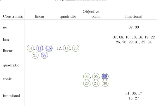
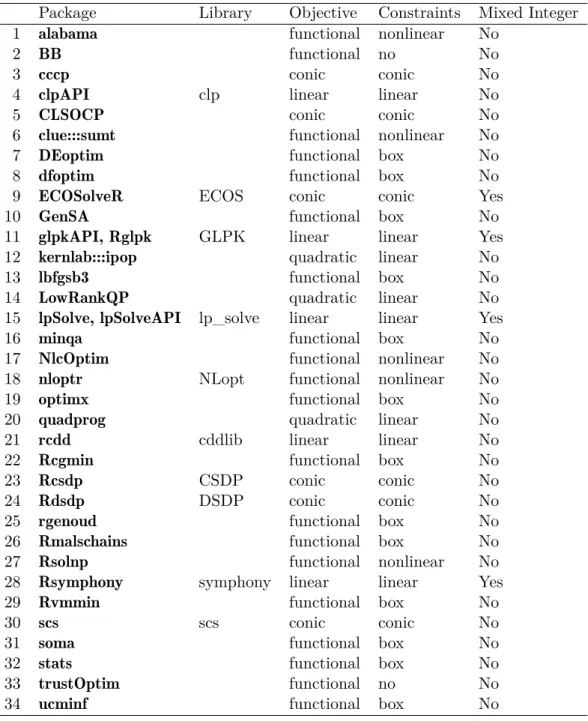
As pointed out in Section 2, in the field of optimization we are typically facing different problem classes. The possibly three most important distinctions are between linear versus nonlinear problems, integer versus continuous and convex versus non-convex problems. Ordered based on increasing complexity, an objective function might be of type linear, (con-vex) quadratic, conic (i.e., any objective expressible as a CP) or functional (i.e., any objective expressible as function). Similarly constraints are typically of type box, linear, (convex) quadratic, conic or functional. Box constraints (or variable bounds) are a special type of

(9)

lin-Objective

Constraints linear quadratic conic functional

no 02, 33 box 07, 08, 10, 13, 16, 19, 22_{25, 26, 29, 31, 32, 34} linear 04 , 11 , 15 12, 14 , 20 21 , 28 quadratic conic 03 , 05 , 09 23 , 24 , 30 functional 01, 06, 17_{18, 27}

Table 1: Overview on optimization problems and solvers.1

ear constraints which enforce lower and upper bounds on the objective variables. The terms conic objective/constraints are used in a general way and refer to any linear and nonlinear ob-jective/constraints that can be reformulated as a conic problem. Therefore this also includes problems with linear and convex quadratic objective/constraints. The most general form are functional objective/constraints which includes all linear and nonlinear objective/constraints. Table 1 gives an overview on which solver can be used to solve which types of OPs. Solvers allowing mixed integer constraints are highlighted with a rectangular frame (e.g., 00) and solvers restricted to convex problems are highlighted with a circular frame (e.g., 00 ). Con-sequently solvers which are restricted to convex problems and can handle integer constraints are marked with both a circular and rectangular frame (e.g., 00 ). For completeness, we note that the linear solvers are also marked to be restricted to convex problems although this is no restriction since all linear problems are convex.

Therefore the position and the frame of a particular solver in the table indicates its ability to solve a given problem. Each problem class to the left and above of the current position can be handled by the solver including its current position. For instance the ECOS(Domahidi, Chu,

and Boyd 2013) solver provided in packageECOSolveR(Fu and Narasimhan 2017, 09 ) is a

convex optimization solver, which can solve conic problems restricted to combinations of the zero, nonnegative, second-oder and primal exponential cone. SinceECOS is equipped with a

branch-and-bound algorithm, it can also be used to solve mixed integer conic problems.

(10)

3.2. Commercial solvers

Since commercial solver packages often bundle a variety of solvers, it is often not possible to assign them to a certain problem class, therefore we will treat them separately. At the time of this writingRinterfaces are available to the commercial solver softwareCPLEX(ILOG 2015), MOSEK (ApS 2017), Gurobi(Gurobi Optimization 2016),Lindo (Lindo Systems 2003) and localsolver(Benoist, Estellon, Gardi, Megel, and Nouioua 2011).

3.3. Non-commercial solvers

The non-commercial solvers landscape can be split into two parts. First, solvers where the functional form is fixed and only the coefficients are provided, this includes all LP, QP, QCQP and CP solvers currently available in R. Second, solvers which can optimize any functional form expressible as an R function. This includes most NLP solvers, sometimes summarized as general purpose solvers.

Linear solvers

Interfaces to several open source LP and MILP solvers are available in R. Most of these packages provide a high-level access to the solver, those explicitly designed to provide a low-level access are commonly marked with the suffixAPI.

The Computational Infrastructure for Operations Research (COIN-OR) project (https:// www.coin-or.org/) provides open-source software for the operations research community. Among this software there are the COIN-OR linear programming (Clp,Forrest, de la Nuez,

and Lougee-Heimer 2004) solver and the SYMPHONY (Ralphs and Güzelsoy 2005, 2011)

solver. Clp is mainly used as library and provides methods for solving LPs via interior point

methods or the simplex algorithm. In R Clp is available through clpAPI (Fritzemeier and

Gelius-Dietrich 2016) which provides a low level interface to Clp. SYMPHONY is a flexible

MILP solver written inC++, that transforms the MILP into LP relaxations to be solved by any LP solver callable through the Open Solver Interface (OSI).Rsymphony(Hornik, Harter,

and Theußl 2017a) provides an interface to theSYMPHONYsolver, where by default the LP

relaxations are solved by theClp solver.

GNU Linear Programming Kit (GLPK,Makhorin 2011) is a solver library written in ANSIC, for solving LP and MILP. InRthe low level interfaceglpkAPI (Fritzemeier, Gelius-Dietrich,

and Luangkesorn 2015) and the high level interface Rglpk (Theußl and Hornik 2017) are

available.

lp_solve(Berkelaar, Eikland, and Notebaert 2016) uses the simplex algorithm combined with

branch-and-bound to solve LPs and MILPs. It furthermore allows to model semi-continuous and special ordered sets problems. PackageslpSolve(Berkelaar 2015) andlpSolveAPI(Konis

2016) provide access to the lp_solvesolver in R.

Additionally the function lpcdd() from package rcdd (Geyer and Meeden 2017) and the

functionsimplex()from packageboot(Canty and Ripley 2017) can be used to solve LPs via

the simplex algorithm.

By taking a closer look at the elements needed by packages capable of solving LPs and MILPs2 we can conclude that the following elements should be present in a consistent and convenient

(11)

optimization infrastructure for modeling LPs and MILPs.

objective: A numeric vector giving the coefficients of the linear objective.

constraints:

• A constraint matrix A (see Equation 3).

• A vector giving the direction of the constraints (i.e., ==,<= or>=). • A vector giving the right hand side b (see Equation3).

bounds: Two vectors giving the lower and upper bounds.

types: A vector storing the type information, i.e., binary, integer and numeric.

maximum: A boolean indicating if the objective function should be maximized or minimized. Although the elements bounds and maximum, as well as the constraint directions and the binary types are not strictly necessary. Their inclusion is motivated by the fact that they are supported by many solvers and simplify the problem specification.

Quadratic solvers

At the time of this writing there exist two non-commercial packages specialized on solv-ing quadratic OPs in R, namely quadprog and LowRankQP. Both are able to solve stricly

convex QPs but can not be used to solve QCQPs. The quadprog (Turlach and

Weinges-sel 2013) package uses the dual method described in Goldfarb and Idnani (1983), whereas

LowRankQP(Ormerod and Wand 2014) is based on an interior point algorithm described in

Fine and Scheinberg(2001).

Additionally, package kernlab (Karatzoglou, Smola, Hornik, and Zeileis 2004; Karatzoglou,

Smola, and Hornik 2016) contains the function ipop() which implements an interior point solver capable of solving QPs.

QP solver generally take the same arguments as LP solver plus an additional matrix parameter storing the coefficients of the quadratic termQ0.

Conic solvers

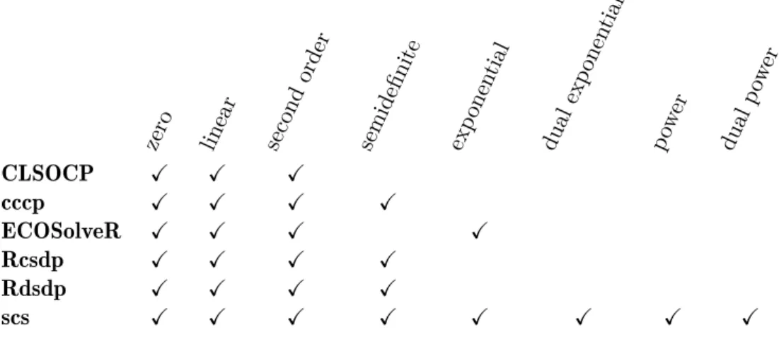
Most of the conic solvers use a standard form similar to Equation 6, where the objective function is assumed to be linear and the vector b−Ax is restricted to a certain cone K. Nevertheless, in Table1they are shown to have a conic objective function and conic constraints to express that they are able to solve any LP and convex NLP expressible by a CP. Therefore, which types of NLPs a given solver can solve, depends on the types of cones the solver can model. Table2 shows the conic solvers available in Rand the types of cones they support. PackageCLSOCP(Rudy 2011) is specialized in solving SOCPs, it is a pureRimplementation of the one-step smoothing Newton method based on the algorithm described in Tang, He, Dong, and Fang (2012). For solving SDP there exist the specialized packages Rcsdp and Rdsdp. Since any SOCP can be transformed into an SDP they can also be used for solving

SOCPs. Rcsdp (Bravo 2016) is an interface to the CSDP (Borchers 1999) library which is

(12)

zero linear second order semidefinite exp onen tial dual exp onen tial power dual power CLSOCP _X _X _X cccp X X X X ECOSolveR X X X X Rcsdp _X _X _X _X Rdsdp X X X X scs X X X X X X X X

Table 2: Conic packages and the supported cones.

and Ye 2008) library. Both packages can read andRcsdpcan also write"sdpa"-files, which is

a file format commonly used to store SDPs. Thecccp(Pfaff 2015) package provides functions

to solve LPs, QPs, SOCPs and SDPs, the algorithms are reported to be similar to those in

CVXOPT(Andersen et al.2016). CVXOPT is aPythonpackage for solving convex OPs via interior-point methods (more information about the algorithms can be found in Andersen, Dahl, Liu, and Vandenberghe 2012). ECOSolveR(Fu and Narasimhan 2017) is an interface

to the embedded conic solver ECOS (Domahidi et al. 2013). A special feature of ECOS is

that it combines convex optimization with branch-and-bound techniques, therefore it can be used to solve CPs where some variables are required to be integer. Thescs(O’Donoghue and

Schwendinger 2016) package is an interface to the Splitting Conic Solver (SCS, O’Donoghue

2015) library, which uses a version of the alternating direction method of multipliers (ADMM) for solving CPs. SCS is designed to solve large cone problems faster than standard

interior-point methods. More information about the algorithm and a comparison to other solvers can be found inO’Donoghue et al.(2016).

General purpose solvers

Solvers capable of handling nonlinear objective functions without further restrictions are called general purpose solvers (GPS). These solvers can minimize (or maximize) any functional form representable as anRfunction with different types of constraints.

Dependent on the solver different types of constraints can be used, where the most general form of constraint is the functional constraint (i.e., any constraint expressible as an R func-tion). The generality of GPS comes at the price of performance and that there is usually no guarantee that a global optimum is reached.

Global GPS Local GPS

Gradient free Gradient Gradient free Gradient

No Constraint 5 0 7 8

Box Constraint 16 4 7 10

Functional Constraint 2 0 7 7

(13)

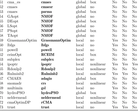
Important properties of GPS are whether they are designed to search for a local or global optima, if gradient information has to be provided or the method is gradient free and which type of constraints can be set. Table3 shows the number of GPS methods grouped by these properties (the counts are based on Table6where additional details can be found) and reveals some interesting details about theRGPS landscape. There exist almost twice as many GPS for local optimization than for global optimization and, even though most of the local solvers utilize gradient information, only four of the global solvers use gradient information. The difference in distribution of gradient based and gradient free optimization algorithms between global and local GPS can be explained by the fact that in global optimization, metaheuristics like evolutionary methods or particle swarm optimization are commonly used. In a recent studyMullen(2014a) surveys the continuous global optimization packages available inRand compares their performance on a set of tests bundled in theglobalOptTests (Mullen 2014b)

package. Table 6 gives an extensive listing of which methods are applicable to global OPs. For more information about the methods we refer toMullen(2014a).

Based on the type of constraints, the GPS can be divided intono constraints,box constraints, linear constraints, quadratic constraints and functional constraints. As Table 3 shows, most of the GPS support no constraint or box constraints. Fortunately, packageoptimx (Nash and

Varadhan 2011) provides a unified interface to many of these solvers, consolidating methods from packagesstats,ucminf(Nielsen and Mortensen 2016),minqa(Bates, Mullen, Nash, and

Varadhan 2014),Rcgmin(Nash 2014b),Rvmmin(Nash 2017) andBB(Varadhan and Gilbert

2009). It was designed as a possible successor ofoptimwhich is part of thestatspackage and

can be used to solve OPs with box constraints. Another package which incorporates many different algorithms is nloptr (Ypma, Borchers, and Eddelbuettel 2017). It is an Rinterface to the NLopt (Johnson 2016) library, which bundles several global and local optimization

algorithms. Depending on the algorithm it can solve NLPs with box-constraints or functional-constraints.

Most of the GPS able to handle functional constraints allow to specify functional equality and/or functional inequality constraints.

To model functional equality constraints the following two forms are most commonly used • hi(x) = 0, i= 1, . . . , k (e.g., alabama (Varadhan 2015), DEoptimR(Conceicao 2016),

nloptr::auglag,nloptr::isres,nloptr::slsqp,NlcOptimand Rnlminb2(Wuertz 2014))

• hi(x) =bi, i= 1, . . . , k (e.g., Rsolnp(Ghalanos and Theussl 2015))

where h is a function and b∈ _Rk _{gives the right hand side. Similarly, functional inequality} constraints are commonly given in one of the following three forms:

• gj(x)≤0, j =k+ 1, . . . , m(e.g., DEoptimR,nloptr::nloptr,NlcOptim(Chen and Yin

2017),Rnlminb2,csr::snomadr(Racine and Nie 2017))

• gj(x)≥0, j =k+ 1, . . . , m(e.g., alabama,nloptr::auglang,

nloptr::auglang, nloptr::cobyla, nloptr::ires, nloptr::mma, neldermead (Bihorel and

Baudin 2015) and nloptr::slsqp)

• lj ≤gj(x)≤uj, j =k+ 1, . . . , m(e.g., ipoptr (Ypma 2011), Rdonlp2(Wuertz 2007),

(14)

where g is a function and l ∈ _Rm−k_, _u _∈

Rm−k are the lower and upper bounds of the constraints. A general optimization infrastructure should be designed in a way that the functional form employed can be transformed into the commonly used forms shown above. An analysis of the above solver spectrum reveals that the critical arguments to GPS are:

start: The initial values for the (numeric) parameter vector.

objective: The function to be optimized.

constraints: Depending on the GPS the constraints can be, none, linear, quadratic, func-tional equality or funcfunc-tional inequality constraints. To model funcfunc-tional constraints consistently with linear and quadratic constraints the following elements are needed.

• A function representing the constraints.

• A vector giving the direction of the constraints. • A vector giving the right hand side.

bounds: Variable bounds, commonly given as lower and upper bounds.

Additionally some GPS make use of the gradient and/or hessian of the objective and the jacobian of the constraints. The optional elements can be summarized by:

gradient: A function that evaluates the gradient of the argument objective.

hessian: A function that evaluates the hessian of the argumentobjective.

jacobian: A function that evaluates the jacobian of the argument constraints.

maximum: A boolean indicating whether the objective function should be maximized or min-imized.

control: Further control arguments specific to the solver. Return values include:

par: The “solution” (parameters) found.

value/objective: The value of the objective function evaluated at the “solution”.

convergence, status: An integer information about the convergence and exit status of the optimization task.

gradient: The gradient evaluated at the solution found.

hessian: The hessian evaluated at the solution found.

message: A text message giving additional information about the optimization / exit status.

(15)

4. A general optimization infrastructure for

R

After reviewing the optimization resources available inR, it is apparent that the main function of a general optimization infrastructure package should take at least three arguments:

problem representing an object containing the description of the corresponding OP, solver specifying the solver to be used (e.g.,"glpk","nlminb","scs"),

control containing a list of additional control arguments to the corresponding solver.

The arguments solver and control are easily understood, since from the available solver spectrum we only have to choose those which are capable to handle the corresponding OP and (optionally) supply appropriate control parameters. However, building the problem object, in a general and intuitive way, seems to be a very challenging task which leads to several design issues.

Based on the review in Sections 2 and 3 it seems natural to instantiate OPs based on an objective function, one or several constraints,types and bounds of the objective variables, as well as the direction of optimization (whether a minimum or a maximum is sought).

4.1. Optimization problem

A new optimization problem is created by calling

OP(objective, constraints, types, bounds, maximum)

where the arguments are explained in detail below.

Alternatively, an OP can be formulated piece by piece, by creating an empty OP

OP()

and using the setter functions to assign the values. The setter and getter functions have the same names as the arguments of OP and can be used to manage specific parts of the OP. For instance, by replacing the linear objective of an LP with a quadratic objective the LP is altered into a QP. An extensive set of examples showing the creation and modification of OPs can be found at the end of this sections.

FunctionOP()always returns an S3 object of class OPwhich stores the entire OP. Storing the OP in a single Robject has many advantages, among others:

• the OP can be checked for consistency during the creation of the problem,

• the different elements of the OP can easily accessed after the creation of the problem, • and the OP can be easily altered, e.g., a constraint can be added, bounds can be

changed, without the need to redefining the entire OP.

(16)

4.2. Objective function

The survey of optimization solvers in Section3 reveals that the way the objective function is stored depends primarily on its functional form. If the objective function is linear (L), i.e.,

a>₀x, then it is common practice to only supply a coefficient vector a0 ∈Rn. For quadratic objective functions (Q) of the form 1

2x

>_Q

0x+a>0x most solvers take a vectora0 ∈Rn and a matrix Q0 ∈Rn×n as input. General nonlinear objective functions (i.e., nonlinear functions which can not be represented as an QP or CP), are represented as an R function (F) which takes the vector of objective variables as argument and returns the objective value. Depending on the type of the objective function, i.e.,F,Q, or Lonly a subset of the solver spectrum can be used.

Objective function types and corresponding constructors implemented inROI are:

F The most general form of an objective function is created with the F_objective(F, n,

G, H, names) constructor by simply supplying F, an R function representing f0(x), and n the length ofx. Optionally, information about the gradient and the hessian can

be provided via the arguments G and H. Is no gradient provided it will be calculated numerically if needed. The optional names argument is propagated to the solution object to make the solution more readable.

Q Objective functions representing a quadratic form as outlined above can be easily created

with the Q_objective(Q, L, names)constructor takingQ, the quadratic partQ0, and optionally L, the linear parta0, as arguments. The namesargument is again optional.

L If the objective to be optimized is a linear function then one should use theL_objective(L,

names)constructor supplyingL(the coefficients to the objective variables) as a numeric vector. The namesargument is again optional.

All three constructors return an object inheriting from class‘objective’. 4.3. Constraints

To model all the problem classes introduced in Section2four different types of constraints are sufficient. Thereby arguments with the same name have the same functionality irrespective of the constraint type hence they are only explained once.

F The most general form of constraints can express any constraint representable by an R function. They are created via F_constraint(F, dir, rhs, J, names), here F is either a function or a list of functions. diris a character vector giving the direction of the constraint and rhsis a numeric vector giving the right hand side of the constraint. The optional arguments J and names can be used to provide the Jacobian and the variable names of the constraints.

C Conic constraints are constructed via the function C_constraint(L, cones, rhs,

names), thereby L can be either a numeric vector of length n or a matrix of

dimen-sion m×n. In accordance with Equation6thecones impose a restriction on the slack

(17)

Q Quadratic constraints as defined in Equation 5can be easily created with the constructor

Q_constraint(Q, L, dir, rhs, names). The quadratic constraints Q are given as a list of lengthm where the entries are either of n×n matrices orNULL.

L Linear constraints are constructed via the functionL_constraint(L, dir, rhs, names).

All constructors return an object inheriting from class‘constraint’.

A conic constraint can be comprised of several cones, where each cone type can occur multiple times. The cone constructors all start withK_followed by an short cut of the cone name, as defined in Section2.3. CurrentlyROIimplements constructors for the conesK_zero,K_nneg,

K_soc, K_psd, K_expp,K_expd,K_powp, and K_powd. To combine different cones the generic combine function c()can be used.

Since in many situations it is desirable to optimize a given objective function subject to a constraint object composed out of different constraints (which may be of different type),ROI

can combine multiple constraints into a single constraint using the generic functions c()or

rbind(). Therefore, the following constraints

L11 x + L12 y = rhs1 L21 x + L22 y ≤ rhs2 L31 x2 + L32 y2 ≤ rhs3

(17) could be formulated in several equivalent ways. First as combination of linear and quadratic constraints R> library("ROI") c(L_constraint(L = rbind(c(L11, L12), c(L21, L22)), dir = c("==", "<="), rhs = c(rhs1, rhs2)), Q_constraint(Q = rbind(c(2 * L31, 0), c(0, 2 * L32)), L = c(0, 0), dir = "<=", rhs = rhs3))

second as combination of linear and conic constraints

c(L_constraint(L = rbind(c(L11, L12), c(L21, L22)), dir = c("==", "<="), rhs = c(rhs1, rhs2)),

C_constraint(L = rbind(c(0, 0), c(-L31, 0), c(0, -L32)), cones = K_soc(3), rhs = c(rhs3, 0, 0)))

or entirely as conic constraints.

C_constraint(L = rbind(c(L11, L12), c(L21, L22), c(0, 0), c(-L31, 0), c(0, -L32)),

cones = c(K_zero(1), K_nneg(1), K_soc(3)), rhs = c(rhs1, rhs2, rhs3, 0, 0))

Additionally the constraints could also be formulated entirely as Q_constraint or

(18)

4.4. Objective variable types

As it is common practice in mixed-integer solvers to distinguish between the variable types continuous, integer and binary we follow this practice. To encode the variable choice charac-ters are used,"C"for continuous,"I"for integer and"B"for binary, where by default all the variables are assumed to be of continuous type.

4.5. Bounds

Variable bounds are a special type of constraints typically used to restrict the objective vari-able between real lower and upper bounds, these are often referred to as “box bounds” or “box constraints”. Although variable bounds could be easily modeled as constraints, most solvers which support any type of constraint also support variable bounds directly. Furthermore, many GPS only support variable bounds as can be seen in Table 3. Thus, it is reasonable but also convenient to consider them separately.

Typically, implementations of optimization algorithms differentiate between five types of ob-jective variable bounds: free (−∞,∞), upper (−∞, ub], lower [lb,∞), double bounded [lb, ub],

and fixed bounds. InROIvariable bounds are represented as a list with two elements—upper

and lower, where only the non-default values are stored in a simple sparse format. In this sparse format only indices and the values of the non-default values are stored. For the lower bounds the default value is zero and for the upper bounds the default value is infinity. Thus for OPs where all the variables are required to take values in the interval [0,∞) no bounds have to be specified. Upper and/or lower bounds are specified by providing the index i of

the corresponding variable (arguments li, ui) and its lower (lb) or upper (ub) bound, re-spectively. Therefore the box constraints −∞ ≤ x1 ≤ 4, 0 ≤ x2 ≤ 100, 2 ≤ x3 ≤ ∞ and 0≤x4≤ ∞ are constructed inROI as follows,

R> V_bound(li = 1:4, ui = 1:4, lb = c(-Inf, 0, 2, 0), + ub = c(4, 100, Inf, Inf))

ROI Variable Bounds:

2 lower and 2 upper non-standard variable bounds.

in the case all the upper and lower values are provided (default values are not omitted) the indices can be left out

R> V_bound(lb = c(-Inf, 0, 2, 0), ub = c(4, 100, Inf, Inf))

2 lower and 2 upper non-standard variable bounds.

in the case default values are omitted the number of objective variables has to be provided.

R> V_bound(li = c(1L, 3L), ui = c(1L, 2L), lb = c(-Inf, 2), ub = c(4, 100), + nobj = 4L)

(19)

2 lower and 2 upper non-standard variable bounds. 4.6. Examples

Here we show how the different types of OPs can be formulated inROI.

LP

Putting all this together, the LP

maximize 3x1 + 7x2 − 12x3 subject to 5x1 + 7x2 + 2x3 ≤61 3x1 + 2x2 − 9x3 ≤35 x1 + 3x2 + x3 ≤31 x1, x2≥0, x3 ∈[−10,10] can be created by R> lp <- OP(objective = L_objective(c(3, 7, -12)), + constraints = L_constraint( + L = rbind(c(5, 7, 2), c(3, 2, -9), c(1, 3, 1)), + dir = c("<=", "<=", "<="), rhs = c(61, 35, 31)),

+ bounds = V_bound(li = 3, ui = 3, lb = -10, ub = 10, nobj = 3), + maximum = TRUE)

R> lp

ROI Optimization Problem:

Maximize a linear objective function of length 3 with - 3 continuous objective variables,

subject to

- 3 constraints of type linear.

- 1 lower and 1 upper non-standard variable bound.

Once an OP is constructed, the functionsobjective(),constraints(),bounds(), types()

and maximum() can be used to access/alter the corresponding element. The function

objective()returns the objective as function, which can be directly used to evaluate param-eters. The number of parameters required, can be obtained by the generic functionlength().

R> param <- rep.int(1, length(objective(lp))) R> objective(lp)(param)

(20)

To access the data of the objective, the generic functionterms()should be used.

R> terms(objective(lp))

$L

A 1x3 simple triplet matrix. $names

NULL

For all the other elements the corresponding getter returns directly the underlying data rep-resentation.

MILP

To extend the LP from above to an MILP, we add the additional requirements x2, x3 ∈ Z, which results in the following OP:

R> milp <- lp

R> types(milp) <- c("C", "I", "I") R> milp

Maximize a linear objective function of length 3 with - 1 continuous objective variable,

- 2 integer objective variables, subject to

- 3 constraints of type linear.

BLP

The following example of a binary linear programming (BLP) problem is based onFischetti and Salvagnin (2010) and will be used later to illustrate how multiple solutions can be ob-tained. minimize −x1−x2−x3−x4−99x5 subject to x1+x2≤1 x3+x4≤1 x4+x5≤1 xi∈ {0,1} (18) R> blp <- OP(objective = L_objective(c(-1, -1, -1, -1, -99)),

+ constraints = L_constraint(L = rbind(c(1, 1, 0, 0, 0), c(0, 0, 1, 1, 0), + c(0, 0, 0, 1, 1)), dir = c("<=", "<=", "<="), rhs = rep.int(1, 3)), + types = rep("B", 5L))

(21)

QCQP

Following the definition from Equation 5, the quadratic terms are multiplied by one-half, therefore the QCQP minimize 1 2(x21+x22) subject to 1 2x 2 1 ≥ 12 x1, x2 ≥0 (19) can be constructed by

R> qcqp <- OP(objective = Q_objective(Q = diag(2), L = c(0, 0)),

+ constraints = Q_constraint(Q = rbind(c(1, 0), c(0, 0)), L = c(0, 0), + dir = ">=", rhs = 0.5))

R> qcqp

Minimize a quadratic objective function of length 2 with - 2 continuous objective variables,

subject to

- 1 constraint of type quadratic.

- 0 lower and 0 upper non-standard variable bounds.

SOCP

For formulating SOCPs it can be advantageous to consider the following alternative standard form (Loboet al. 1998;Andersenet al. 2012),

minimize a>₀x

subject to kBix+wik2 ≤u>i x+vi, i= 1, . . . , k (20) here k is the number of second-order cones,Bi ∈R(di−1)×n,wi∈Rdi−1,ui∈Rn,vi ∈R and the dimension of each cone is given bydi. Starting from Equation20the transformation into the standard form given in Equation6 can be accomplished by

A=−         u>₁ B1 ... u>_k Bk         , b=         v1 w1 ... vk wk         , s∈ Y i=1,...,k Kdi soc. (21) Therefore the OP maximize x+y+z subject to √x2+_z2_≤√2 x, y, z ≥0, y≤5 (22) can be easily solved inROI.

(22)

R> socp <- OP(objective = L_objective(c(1, 1, 1), names = c("x", "y", "z")), + constraints = C_constraint(rbind(c(0, 0, 0), c(-1, 0, 0), c(0, 0, -1)), + cones = K_soc(3), rhs = c(sqrt(2), 0, 0)),

+ bounds = V_bound(ui = 2, ub = 5, nobj = 3L), maximum = TRUE) R> socp

Maximize a linear objective function of length 3 with - 3 continuous objective variables,

subject to

- 3 constraints of type conic.

|- 3 conic constraints of type 'soc'

Similarly by making use of the epigraph form (see Equation 7, the convex QP minimize qx2₁+x2₂

subject to x1+x2= 2 x1, x2≥0

(23) can be formulated as a SOCP.

R> A <- rbind(c(0, 0, -1), c(-1, 0, 0), c(0, -1, 0), c(1, 1, 0)) R> b <- c(1, 0, 0, 2)

R> cp <- OP(objective = L_objective(c(0, 0, 1)),

+ constraints = C_constraint(A, c(K_soc(3), K_zero(1)), b)) R> cp

Minimize a linear objective function of length 3 with - 3 continuous objective variables,

subject to

|- 3 conic constraints of type 'soc' |- 1 conic constraint of type 'zero'

SDP

Another standard form commonly used for SDPs (e.g., Vandenberghe and Boyd (1996b);

Nemirovski(2004); Andersenet al. (2012)) is

minimize a>₀x

subject to Pn

(23)

here a0 ∈ Rn and Fi ∈ Rd×d are symmetric matrices and is the generalized inequality. ThereforePn

i=1xiFi F0 is equivalent to F0−Pni=1xiFi ∈ Kd_psd. In order to transform an SDP problem given in the form of Equation 24 into the form shown in Equation 6, a half-vectorization should be performed. Half-half-vectorization is a special kind of matrix half-vectorization for symmetric matrices, which transforms a symmetric matrix

R> (A <- matrix(c(1, 2, 3, 2, 4, 5, 3, 5, 6), nrow = 3))

[,1] [,2] [,3]

[1,] 1 2 3

[2,] 2 4 5

[3,] 3 5 6

into a vector, alikevechtransformsnsymmetricd×dmatrices into a (d(d+1)/2)×nmatrix:

R> vech(A) [,1] [1,] 1 [2,] 2 [3,] 3 [4,] 4 [5,] 5 [6,] 6

Specifically, the following problem minimize x1+x2−x3 subject to x1 10 3_{3 10} ! +x2 6 −4 −4 10 ! +x3 8 1_{1 6} ! 16 −13 −13 60 ! x1, x2, x3≥0 can be modeled as follows:

R> F1 <- rbind(c(10, 3), c(3, 10)) R> F2 <- rbind(c(6, -4), c(-4, 10)) R> F3 <- rbind(c(8, 1), c(1, 6))

R> F0 <- rbind(c(16, -13), c(-13, 60))

R> psd <- OP(objective = L_objective(c(1, 1, -1)),

+ constraints = C_constraint( L = vech(F1, F2, F3), cone = K_psd(3), + rhs = vech(F0)))

R> psd

Minimize a linear objective function of length 3 with - 3 continuous objective variables,

(24)

subject to

|- 3 conic constraints of type 'psd'

NLP

The following example fromRosenbrock(1960) is some times referred to as Rosenbrock’s post office problem. maximize x1x2x3 subject to x1+ 2x2+ 2x3 ≤72 x1, x2, x3 ∈[0,42] (25) R> nlp_1 <- OP()

R> gradient <- function(x) c(prod(x[-1]), prod(x[-2]), prod(x[-3]))

R> objective(nlp_1) <- F_objective(F = function(x) prod(x), n = 3, G = gradient) R> rosenbrock <- function(x) x[1] + 2 * x[2] + 2 * x[3]

R> constraints(nlp_1) <- F_constraint(F = rosenbrock, dir = "<=", rhs = 72, + J = function(x) c(1, 2, 2))

R> bounds(nlp_1) <- V_bound(ud = 42, nobj = 3L) R> maximum(nlp_1) <- TRUE

R> nlp_1

Maximize a nonlinear objective function of length 3 with - 3 continuous objective variables,

subject to

- 1 constraint of type nonlinear.

Alternatively the linear constraintx1+ 2x2+ 2x3≤72 could and should be modeled directly as a linear constraint,

R> nlp_2 <- nlp_1

R> constraints(nlp_2) <- L_constraint(L = c(1, 2, 3), "<=", 72) R> nlp_2

Maximize a nonlinear objective function of length 3 with - 3 continuous objective variables,

subject to

- 1 constraint of type linear.

(25)

using L and Q constraints rather than F_constraint has the advantage that for L and Q

constraints the Jacobian is derived analytically if needed and not provided.

5. Package

ROI

The R optimization infrastructure can be structured into the package ROI and its

accom-panying extensions. Package ROI provides all the necessary classes, methods and manages

the extensions. The extension packages add optimization solvers, read/writing functions and additional resources (e.g., model collections). Currently ROI distinguishes between two

dif-ferent types of extensions, namely, plug-ins and models. Here plug-ins play a special role, hence all plug-ins are loaded automatically when ROI is loaded. When a plug-in is loaded

it provides data about its capabilities. This data is stored in an in-memory database and includes information about to which problems the plug-in is applicable, which formats it can read/write and the control arguments available from the solver and how the solver specific control arguments relate to arguments commonly used.

This mechanism makes it possible that ROIis aware of all the installed plug-ins, without the

need to change ROI when a new plug-in is added. To make the automatic loading possible

the plug-ins have to follow the name convention ROI.plugin.<name>, where <name> is typically the name of an optimization solver (e.g., ROI.plugin.glpk (Theussl 2017)). The

prefix ROI.models (e.g., ROI.models.netlib (Schwendinger 2016)) is used for data packages

with predefined OPs. In Section 5.6 we give an overview about the data packages available in the ROIformat.

5.1. Solving optimization problems

After formulating an OP as described in Section 4, it can be solved by calling the func-tion ROI_solve(x, solver, control, ...). This function takes an R object of class OP containing the formulation of the OP, the name of the solver to be used and a list con-taining solver-specific parameters as arguments. The solver and control arguments are optional, if no solverargument is provided ROIwill choose an applicable solver

automati-cally (see Section 5.7.1). Alternatively the solver-specific parameters can be specified via the dots arguments.

R> lp_sol <- ROI_solve(lp, solver = "glpk") R> lp_sol

Optimal solution found.

The objective value is: 8.670149e+01

R> milp_sol <- ROI_solve(milp, solver = "symphony") R> milp_sol

R> blp_sol <- ROI_solve(blp, solver = "glpk") R> blp_sol

(26)

The objective value is: -1.010000e+02

R> socp_sol <- ROI_solve(cp, solver = "ecos") R> socp_sol

The objective value is: 4.142136e-01

R> psd_sol <- ROI_solve(psd, solver = "scs") R> psd_sol

R> nlp_1_sol <- ROI_solve(nlp_1, solver = "alabama", start = c(10, 10, 10)) R> nlp_1_sol

Some OPs have multiple solutions, in the case of BLP (MILP) some solver can retrieve all (multiple) solutions. For MILPs it is in general not possible to obtain all the solutions but only multiple solutions, since even this simple MILP

minimize x1−x2 subject to x1−x2= 0 x1, x2∈Z

(26) has an infinite number of solutions. In the following we use the"msbinlp" solver to retrieve all the solutions to the OP defined in Equation18, here methodgives the solver used within the inner loop andnsol_maxthe maximal number of solutions to be returned. Since we have a pure binary problem and five objective variables, it is clear that there can be at most ten solutions,

R> blp_sol <- ROI_solve(blp, solver = "msbinlp", method = "glpk", nsol_max = 10) R> blp_sol

2 optimal solutions found.

alternatively it is also possible to set nsol_max to Inf. Then ROI tries to retrieve all the

solutions.

5.2. Solution and status code

To make the solutions of the various solvers easy to understand, all the solutions are canon-icalized within the plug-ins. After the canonicalization each solution contains the following components:

(27)

solution the solution of the OP,

objval the optimal objective value,

status the canonicalized status code,

message the original solver message

and a meta attribute containing the solver name and additional optional arguments.

Solver status codes are used to inform the user about the exit status of the solver. Despite the common usage of status codes in optimization solvers there is no widely used standard. Nevertheless, we believe it is desirable to provide unified status codes. The status codes used in ROI_solve are simple and consistent with the common practice, to return 0

on success (if a “solution” meeting the solver specific requirements was found) 1otherwise. To obtain the (primal) “solution” the generic function solution(x, type) should be used,

R> solution(lp_sol)

[1] 0.000000 9.238806 -1.835821

in the case of multiple solutions a "list"of solutions is returned.

R> solution(blp_sol)

[[1]]

[1] 0 1 1 0 1 [[2]]

[1] 1 0 1 0 1

If the status code is 1 solutionwill return NA, to prevent the user from using solutions with a status code different from 0.

R> lp_inaccurate_sol <- ROI_solve(lp, solver = "scs", tol = 1e-32) R> solution(lp_inaccurate_sol)

[1] NA NA NA

However in a few situations it can be desirable to obtain solutions even if the solver signals no success. In these cases ROI can be forced to return the solution provided by the solver

regardless of the status code.

R> solution(lp_inaccurate_sol, force = TRUE)

[1] 8.142725e-16 9.238806e+00 -1.835821e+00

(28)

R> solution(lp_sol, type = "dual")

[1] -4.298507 0.000000 0.000000

Furthermore, auxiliary variables

R> solution(lp_sol, type = "aux")

$primal

[1] 61.0000 35.0000 25.8806 $dual

[1] 0.5820896 1.4626866 0.0000000

the solution matrices of a PSD problem

R> lapply(solution(psd_sol, type = "psd"), as.matrix)

$`4`

[,1] [,2]

[1,] 0.11050022 0.031337481 [2,] 0.03133748 0.008887201

the original solver message

R> solution(lp_sol, type = "msg") $optimum [1] 86.70149 $solution [1] 0.000000 9.238806 -1.835821 $status [1] 5 $solution_dual [1] -4.298507 0.000000 0.000000 $auxiliary $auxiliary$primal [1] 61.0000 35.0000 25.8806 $auxiliary$dual [1] 0.5820896 1.4626866 0.0000000

(29)

R> solution(lp_sol, type = "objval")

[1] 86.70149

the status

R> solution(lp_sol, type = "status")

$code [1] 0 $msg solver glpk code 5 symbol GLP_OPT

message Solution is optimal. roi_code 0

and the status code

R> solution(lp_sol, type = "status_code")

[1] 0

of the OP can be retrieved by the functionsolution(). 5.3. Reformulations

Reformulations are often used to transform a problem of class A into a problem of class B, where the solution of the original problem can be derived from the solution of the reformulation (which is typically easier to solve). Although reformulation tech-niques are commonly used in optimization the functions performing these reformula-tions are generally hidden within the optimization software. To facilitate the compari-son of different reformulation algorithms ROI provides functions for managing

reformula-tions. Function ROI_registered_reformulations() lists the available reformulations and

ROI_reformulate(x, to, method)performs the reformulation. Following Boros and Ham-mer (2002) we illustrate the transformation of a binary QP into a MILP, the code for the reformulation is based on the implementation in therelations(Meyer and Hornik 2017)

pack-age.

minimize 6−x−4y−z+ 3xy+yz

x, y, z ∈ {0,1} (27)

R> Q <- rbind(c(0, 3, 0), c(0, 0, 1), c(0, 0, 0))

R> bqp <- OP(Q_objective(Q = Q + t(Q), L = c(-1, -4, -1)), types = rep("B", 3)) R> glpk_signature <- ROI_solver_signature("glpk")

(30)

objective constraints bounds cones maximum C I B

1 L X X X TRUE TRUE FALSE FALSE

2 L L X X TRUE TRUE FALSE FALSE

3 L X X X TRUE FALSE TRUE FALSE

R> milp <- ROI_reformulate(x = bqp, to = glpk_signature) R> ROI_solve(milp, solver = "glpk")

HereROI selects the applicable reformulations based on the provided signatures. A method

is considered to be applicable if it can transform the given OP into a new OP, where the signature of the new OP is a subset of the signature provided in the argument to. Since it is possible that several methods are applicable, the argumentmethodcan be used to select a specific reformulation method.

5.4. ROI solvers

ROI currently can make use of eighteen different solvers, applicable to a wide range

of OPs. Inspired by R’s available.packages() function, ROI can return a listing of

the solver plug-ins available at CRAN (https://CRAN.R-project.org), R-Forge (https:

//r-forge.r-project.org/,Theußl and Zeileis 2009) and GitHub(https://github.com/). ROI_available_solvers()without an argument lists all the available solvers. If an OP is provided as argument, only the available solvers applicable will be returned.

R> ROI_available_solvers(cp)[, c("Package", "Repository")]

Package Repository

4 ROI.plugin.ecos https://cran.r-project.org/src/contrib 12 ROI.plugin.scs https://cran.r-project.org/src/contrib 17 ROI.plugin.ecos http://R-Forge.R-project.org 27 ROI.plugin.scs http://R-Forge.R-project.org

A listing of all the available plug-ins on CRANand R-Forgecould be easily compiled by just using theavailable.packages()function. But to be able to find all the solvers available and applicable to a given OP also the solver signature is needed. Therefore a database containing the solver signatures and the information provided by available.packages was compiled and is queried wheneverROI_available_solvers is called.

A vector of all solvers installed and loaded (registered) can be obtained by,

R> ROI_registered_solvers()

nlminb alabama cbc

"ROI.plugin.nlminb" "ROI.plugin.alabama" "ROI.plugin.cbc"

clp cplex deoptim

(31)

ecos glpk gurobi "ROI.plugin.ecos" "ROI.plugin.glpk" "ROI.plugin.gurobi"

ipop lpsolve mosek

"ROI.plugin.ipop" "ROI.plugin.lpsolve" "ROI.plugin.mosek"

msbinlp nloptr optimx

"ROI.plugin.msbinlp" "ROI.plugin.nloptr" "ROI.plugin.optimx"

quadprog scs symphony

"ROI.plugin.quadprog" "ROI.plugin.scs" "ROI.plugin.symphony"

similarly

R> ROI_applicable_solvers(cp)

[1] "ecos" "scs"

returns a vector giving the names of the registered solvers applicable to a given problem. Both return values are based on the solver registry, which stores the solver method and information about the solver registered by the plug-ins. The solver registry is an in-memory database based on theregistry (Meyer 2015) package.

ROI_installed_solvers gives a listing of all the installed plug-ins (not necessarily loaded) delivered directly with ROIand found

R> ROI_installed_solvers()

nlminb alabama cbc

"ROI.plugin.nlminb" "ROI.plugin.alabama" "ROI.plugin.cbc"

clp cplex deoptim

"ROI.plugin.clp" "ROI.plugin.cplex" "ROI.plugin.deoptim"

ecos glpk gurobi

"ROI.plugin.ecos" "ROI.plugin.glpk" "ROI.plugin.gurobi"

ipop lpsolve mosek

"ROI.plugin.ipop" "ROI.plugin.lpsolve" "ROI.plugin.mosek"

msbinlp nloptr optimx

"ROI.plugin.msbinlp" "ROI.plugin.nloptr" "ROI.plugin.optimx"

quadprog scs symphony

"ROI.plugin.quadprog" "ROI.plugin.scs" "ROI.plugin.symphony"

by searching for the prefix ‘ROI.plugin’ in the Rlibrary trees.

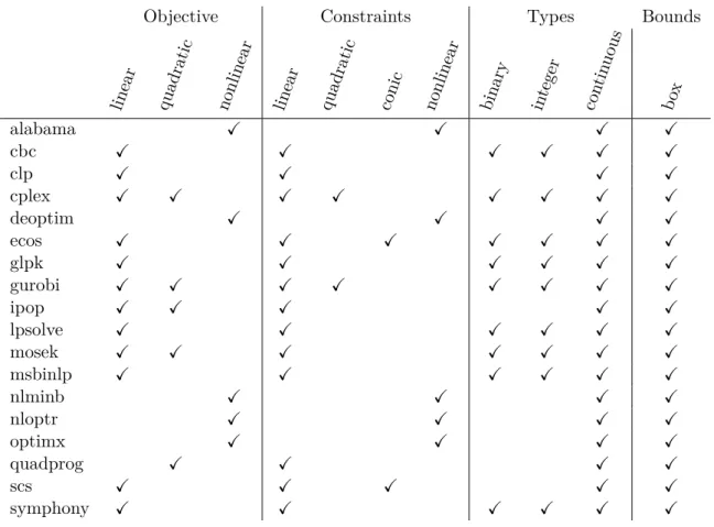
An overview on the currently available solver plug-ins based on the problem types is given in Table4. Please note that the functionality provided in a plug-in does not necessarily have to be the same as the functionality of the solver, e.g.,ROI.plugin.nlminb can take functional

constraints nlminb can only take box constraints. Furthermore we want to emphasize that ROIwas built to be extended, as shown in Section6.

5.5. ROI read/write

OPs are commonly stored in flat file formats, different solvers allow to read/write different types of this file formats. ROI manages the reader/writer registered in the plug-ins, thus

(32)

Objective Constraints Types Bounds

linear quadratic nonlinear linear quadratic conic nonlinear binary integer con tinuous box alabama X X X X cbc X X X X X X clp X X X X cplex X X X X X X X X deoptim X X X X ecos X X X X X X X glpk X X X X X X gurobi X X X X X X X X ipop X X X X X lpsolve X X X X X X mosek X X X X X X X msbinlp X X X X X X nlminb X X X X nloptr X X X X optimx X X X X quadprog X X X X scs X X X X X symphony X X X X X X

Table 4: Currently available ROIplugins.

R> lp_file <- tempfile()

R> write.op(lp, lp_file, "lp_lpsolve") R> writeLines(readLines(lp_file)) /* Objective function */ max: +3 C1 +7 C2 -12 C3; /* Constraints */ +5 C1 +7 C2 +2 C3 <= 61; +3 C1 +2 C2 -9 C3 <= 35; +C1 +3 C2 +C3 <= 31; /* Variable bounds */ -10 <= C3 <= 10; and read R> read.op(lp_file, "lp_lpsolve")