Structure exploiting optimization methods for model predictive control

(1)

Thesis for theDegree ofDoctor ofPhilosophy

Structure exploiting optimization

methods for model predictive control

E

_mil

K

_lintberg

Department of Signals and Systems ChalmersUniversity ofTechnology

(2)

Structure exploiting optimization methods for model predictive control EmilKlintberg

ISBN 978-91-7597-567-2 c

EmilKlintberg, 2017.

Doktorsavhandlingar vid Chalmers tekniska högskola Ny serie nr 4248/2017

ISSN 0346-718X

Department of Signals and Systems ChalmersUniversity ofTechnology

SE–412 96 Göteborg Sweden

Telephone: +46 (0)31 – 772 1000 Email: [email protected]

Typeset by the author using LA_TEX.

Chalmers Reproservice Göteborg, Sweden 2017

(3)

Abstract

This thesis considers optimization methods for Model Predictive Control (MPC). MPC is the preferred control technique in a growing set of applications due to its flexibility and to the natural way in which constraints can be incorporated in the control policy. Its applicability is, however, limited by the high computational burden associated with the solution of the underlying optimization problems. To alleviate this drawback we study structures in the MPC problems, which can enhance their solution.

The first topic of the thesis is numerical structures in matrices arising in gradient-based optimization methods for MPC. The idea is that due to the nu-merical structures, dense matrices can be approximated by sparse matrices to reduce the computational cost per iteration, and also for the overall solution of the MPC problem.

The second topic of the thesis is parallelizable optimization methods for multi-stage MPC. Multi-stage MPC is a popular framework used to increase the robustness of MPC schemes. One major drawback, however, is that the under-lying optimization problems become very large. In this context, we consider parallel implementations of two different classes of optimization methods. First, we propose a parallelizable linear algebra for a primal-dual interior point method for two-stage MPC problems, i.e. for multi-stage MPC problems where the sce-nario tree is restricted to only branch in its root node. Secondly, we consider Newton’s method to solve the Lagrange dual problem of multi-stage MPC prob-lems. We show that the Hessian of the dual function is permutation similar to a block-tridiagonal matrix, propose a strategy for reducing the need for regular-ization, and reduce the cost of globalization strategies for problems with simple constraints and a diagonal cost.

The third topic of the thesis is optimization methods for solving distributed MPC problems in a distributed fashion using dual decomposition. Dual decom-position is commonly used with gradient-based methods to achieve a completely distributed method. In this thesis, however, we use dual decomposition together with Newton’s method to achieve semi-distributed methods with a fast practi-cal convergence. We study the occurence of a singular dual Hessian and pro-pose a constraint relaxation to prevent it. Additionally, we propro-pose a distributed dual Newton strategy which can be viewed as a distributed primal-dual interior point method, and study the numerical structure of the dual Hessian for prob-lems stemming from MPC deployed on multi-agent systems that are interacting via non-delayed couplings.

(4)

Abstract

Keywords: Model Predictive Control, Multi-stage robust MPC, Distributed op-timization, Optimization methods.

(5)

Acknowledgments

As my time as a PhD student is coming to an end, it is time to acknowledge some of the people that have offered support on the way.

First, I would like to express my gratitude towards Bo Egardt for giving me the opportunity to start as a PhD student in his group. In hindsight, this was a crossroad in my career where I believe that I chose the right path.

I have also been lucky to have many fruitful and enjoyable collaborations during my time at Chalmers. I have learned a lot about optimization from my supervisor Sebastien Gros. Moritz Diehl has hosted me twice, once in Leuven and once in Freiburg, where I have had the opportunity to collaborate with Attila Kozma and Dimitris Kouzoupis. At Chalmers I had the opportunity to collab-orate with John Dahl and Anton Klintberg. I am very thankful for all these collaborations.

Last and most importantly, I would like to express my gratitude towards my family and friends.

Emil Klintberg Göteborg, April 2017

(6)

(7)

List of publications

This thesis is based on the following seven appended papers.

Standard MPC

Paper 1

Emil Klintberg, Sebastien Gros. Approximate inverses in precon-ditioned fast dual gradient methods for MPC. Accepted to the 20th IFAC World Congress, July 2017.

Multi-stage MPC

Paper 2

Emil Klintberg, Sebastien Gros. A Parallelizable Interior Point Method for Two-Stage Robust MPC. IEEE Transactions on Control Systems Technology, vol. PP, 2017.

Paper 3

Emil Klintberg, John Dahl, Jonas Fredriksson, Sebastien Gros. An improved dual Newton strategy for scenario-tree MPC.IEEE Con-ference on Decision and Control, pp. 3675-3681, December 2016.

Paper 4

Emil Klintberg, Dimitris Kouzoupis, Moritz Diehl, Sebastien Gros. A dual Newton strategy with fixed iteration complexity for multi-stage MPC.Technical report. CPL Publication id: 248820. Chalmers University of Technology.

(8)

List of publications

Distributed MPC

Paper 5

Attila Kozma, Emil Klintberg, Sebastien Gros, Moritz Diehl. An Improved Distributed Dual Newton-CG Method for Convex Quadratic Programming Problems. American Control Conference, pp. 2324-2329, July 2014.

Paper 6

Emil Klintberg, Sebastien Gros. A Primal-Dual Newton Method for Distributed Quadratic Programming. IEEE Conference on De-cision and Control, pp. 5843-5848, December 2014.

Paper 7

Emil Klintberg, Sebastien Gros. Numerical structure of the Hes-sian of the Lagrange dual function for a class of convex problems. SIAM Journal on Control and Optimization, vol. 55, issue 1, pp. 574-593, 2017.

Other publications

In addition to the appended papers, the following papers are also written by the author of the thesis.

Emil Klintberg, Sebastien Gros. An inexact interior point method for optimization of differential algebraic systems. Computers and Chemical Engineering, vol. 92, pp. 163-171, 2016.

Anton Klintberg, Emil Klintberg, Björn Fridholm, Hannes Kuu-sisto, Torsten Wik. Statistical modeling of OCV-curves for aged battery cells.Accepted to the 20th IFAC World Congress, July 2017.

(9)

Notations and abbreviations

Notation Meaning

R Set of real numbers

[a,b] Interval of real numberszsuch thata≤z≤ b

(a,b) Interval of real numberszsuch thata<z< b

Rm×n Set of real matrices of dimensionm×n

Sn Set of symmetric real matrices of dimensionn×n

Sn₊ Set of symmetric positive semidefinite matrices of dimensionn×n

Sn₊₊ Set of symmetric positive definite matrices of dimensionn×n

A0 The matrixAis positive definite

A0 The matrixAis positive semidefinite

diag(a1, . . . ,an) Diagonal matrix with diagonal elementsa1, . . . ,an

1 Column vector of ones

∂f

∂z ∈R n×m

Jacobian of the function f :Rm →Rnwith respect to the variablez ∇f ∈_Rm×n _{Gradient of the function}

f :_Rm _→ Rn

∇2f ∈_Sn _{Hessian of the function} _f _:

Rn→ R

dom f Domain of the function f :_Rn_→

R

Abbreviation Meaning

CQ Constraint Qualification

CPU Central Processing Unit

KKT Karush-Kuhn-Tucker

LICQ Linear Independence Constraint Qualification

min minimize

MPC Model Predictive Control

QP Quadratic Program

s.t. subject to

(10)

(11)

3.1 Numerical structure of the dual Hessian . . . 182 3.2 A distributed quasi-Newton strategy . . . 188 4 Extension to inequality constrained problems . . . 191 4.1 Dual decomposition using the relaxed dual function . . . 192 5 Numerical experiments . . . 197 6 Conclusions and future research directions . . . 198 References . . . 200

(16)

(17)

Part I

(18)

(19)

Chapter 1 Introduction

This chapter provides a brief background on Model Predictive Control (MPC). The concepts of robust MPC and distributed MPC are also introduced, and the main contributions of the thesis are summarized.

1.1 Background

In the early 1970s, it was observed that the performance of the complex and multivariable systems in process industry could be improved by using predictive, receding horizon controllers. Several control techniques were proposed where the arguably most well-known is the so-called Dynamic Matrix Control (DMC) developed at Shell Oil [1].

In DMC, a linear step response of the system was repeatedly simulated over a finite horizon and optimal control actions were calculated as the solution to a least-squares problem. Due to the simulation, unusual dynamic behaviors could be forecasted and complex control problems, which were unsolvable with PID controllers, could be handled. In its first version, the DMC was unable to incor-porate system constraints in the control law, although this was later addressed by formulating the problem as a Quadratic Program (QP) [2]. The ability of han-dling system constraints was particularly important, since the economically most beneficial operating point of processing units is often located at the intersection of constraints [3].

The early receding horizon controllers, such as the DMC controller, are di-rect ancestors of modern MPC, which nowadays is the preferred control tech-nique in a growing set of applications. In MPC, control actions are repeatedly calculated to optimize the predicted system behaviour, and the benefits over tra-ditional control techniques are thus inherited from the DMC. In addition to its practical benefits, an important research effort has been dedicated to develop a rigorous theoretical foundation for MPC controllers [4].

(20)

Chapter1. Introduction

However, the benefits compared to traditional control techniques come at the expense of solving an optimization problem at every sampling instant. This weakness initially limited the use of MPC to systems with long sampling times and to applications where expensive computing units could be afforded. Hard-ware improvements and an intensive research effort to design tailor-made opti-mization techniques have, however, alleviated these drawbacks and have made MPC feasible for increasingly faster systems and for some embedded applica-tions. Despite the improvements, MPC is still intractable or very challenging in many demanding applications.

In the following sections, we provide an overview of optimization methods for MPC, and introduce two challenging problem classes; robust MPC and dis-tributed MPC.

1.2 Overview of optimization techniques for MPC

In the early 2000s, so-calledexplicit MPCwas proposed where the optimization problem is solved offline and the result is saved as a look-up table for online use [5]. This strategy quickly proved to be useful in some challenging applications and earned a significant attention in the literature [6–9]. However, the approach is in general limited to short horizons and linear systems with few states due to the excessive memory requirements otherwise. The significance of explicit MPC has therefore decreased with the development of customized online optimization methods, although some recent results have been directed towards reducing the memory requirements of the method [10].

Interior point methodsare often preferred due to their robustness, practically consistent convergence and their polynomial (although not necessarily tight) bounds on the runtime. An early interior point method that exploited the spe-cific structure of optimization problems arising from MPC was proposed in [11]. The method used a Riccati recursion to find the search directions and showed a linearly increasing computational cost with the horizon, compared to a cubically increasing cost for a naive implementation. After this, a variety of tailor-made in-terior point methods with decreasing runtimes [12–15] and computational com-plexities [16] have followed.

It has also been proposed to exploit the similarity between subsequent opti-mization problems in MPC by using anactive set method. Specifically, based on the preceding problem a good initial guess for the active set can be provided, which often significantly improves the convergence of the method. This idea was successfully implemented in [17], and further exploited in [18,19] where a paral-lelizable method was presented. However, active set methods lack the practically consistent convergence of interior point methods, and have no useful bound on the runtime.

(21)

1.3. RobustMPC

A considerable part of the recent developments has been devoted to first-order methods. In particular the Alternating Direction Method of Multipliers [20] and the fast gradient method [21–25] are commonly identified as favourable for embedded MPC. Their popularity is stemming from their easy implementa-tion and from the fact that, in contrast to interior point methods and active set methods, they have practically useful bounds on the runtime. However, their practical performance is heavily affected by the problem data. This is partly alle-viated by the generalized fast gradient method which was presented in [26], and used in the context of MPC in [27, 28].

1.3 Robust MPC

An important property of a control system is its ability of handling plant vari-ations and uncertainties, i.e. its so-called robustness. Being a feedback control technique, MPC has in its linear case some intrinsic robustness [29, 30]. Con-straint satisfaction can, however, not be guaranteed if uncertainties are present in the system, and in the case of nonlinear systems the resulting control scheme may be non-robust [30]. As a remedy, several formulations of robust MPC schemes have been proposed to handle uncertainties in the employed model.

The early formulations of robust MPC used a min-max formulation [31], where the worst-case of several possible output trajectories was optimized, while the control inputs were feasible for all possible realizations of the uncertainty. It was, however, observed that the formulation could lead to infeasible optimization problems and was overly conservative, since it did not consider the fact that a new problem would be solved at the next sampling instant.

To account for the feedback, it was proposed to perform the optimization over feedback control laws instead of control inputs [32]. The resulting opti-mization problem was, however, infinite dimensional and thus difficult to solve. Several approximations were proposed to obtain a tractable formulation, includ-ing so-calledtube-based MPCwhere the feedback law is approximated around a nominal trajectory [33, 34].

Another formulation which has recently gained attention in the literature is the so-called multi-stage MPC [35, 36]. Stemming from the field of stochas-tic programming, this formulation represents the uncertainty by a scenario tree, which in contrast to the early min-max formulations accounts for the feedback in the MPC scheme. A major drawback, however, is that the size of the underlying optimization problem grows exponentially with the length of the horizon. To alleviate this, several tailor-made optimization techniques have been proposed.

An early interior point method that exploits the specific structure of optimiza-tion problems originating from scenario tree problems was proposed in [37]. The method uses a Riccatti recursion to calculate the search direction in normal

(22)

tion form, and supports a certain degree of parallelism. Later, it has been pro-posed to use dual decomposition to achieve parallelizable methods that exploit the specific structure of multi-stage MPC problems. In [38], dual decomposi-tion is used in conjuncdecomposi-tion with a first-order method whereas in [39] a Newton strategy is used in the dual space.

1.4 Distributed MPC

Many large scale systems are composed of interacting subsystems, which for various reasons are hard to control with a central controller. It is then natural to consider distributed control techniques.

Distributed MPC has for the last 10 years been a popular field of research, which has resulted in a vast collection of methods, where a significant part in-volves local MPC controllers of each subsystem. Methods of this kind are com-monly categorized asdecentralized [40, 41] if no communication between the subsystems is used, or in the case of communication ascooperative [42, 43] or non-cooperative[44–46] depending on the local objective functions.

Another strategy to achieve a distributed MPC controller, which we will fo-cus on, is to rely on techniques from distributed optimization to solve the central MPC optimization problem. Although the large-scale optimization problem can be very challenging to solve in real-time, this formulation has the obvious advan-tage of not sacrificing control performance compared to central control. For this purpose, several methods have been proposed, mostly based on so-calledprimal decompositionordual decomposition.

In primal decomposition, the optimization problem is split into a two level problem, where the local variables are manipulated locally, and the shared vari-ables are manipulated via a so-called master problem. As a result, the iterates are feasible after every iteration, but the approach generally suffers from an in-creasing number of variables in the master problem for an inin-creasing number of subsystems. Several methods using primal decomposition for MPC have been proposed in the literature, see e.g. [47–49].

In dual decomposition, the optimization problem is also split into a two level problem, where all primal variables are manipulated locally and the subproblems are coordinated via the dual variables which are adjusted in a master problem. In this case, the number of variables in the master problem is usually not increasing as rapidly with the number of subsystems, but the iterates are not feasible until convergence is achieved. This strategy was first proposed for distributed MPC in [50, 51], and has then been proposed in conjunction with a variety of methods [52–55] and for a variety of applications [56].

(23)

1.5. Motivation and contributions

1.5 Motivation and contributions

Despite the immense algorithmic research, further improvements are still needed to extend the use of MPC to fast systems that in addition are embedded, large-scale, safety critical, uncertain or in some other way complicated. The diffi -culty lies in extending methods to have seemingly conflicting properties, as e.g. possessing a fast and consistent practical convergence besides being scalable or having tight bounds on the runtime.

The focus of this thesis is on optimization methods for MPC, where the main contributions can be divided into methods for standard MPC, multi-stage MPC, and for distributed optimization, which can be used to form distributed MPC schemes. The contribution for standard MPC aims at decreasing the computa-tional cost of a first-order method and hence to facilitate the usage of MPC in embedded applications. The contributions for multi-stage MPC and distributed MPC aim at improving the scalability of interior-point methods and active set methods for these problem classes. The main contributions are outlined below.

1.5.1 Standard MPC

It is commonly proposed to use first-order methods to solve the Lagrange dual problem in the context of MPC. However, the methods are in general sensitive to ill-conditioning. In [28], this drawback is resolved at the expense of more computationally demanding iterations by using a preconditioned fast gradient method. In the paper:

Emil Klintberg, Sebastien Gros. Approximate inverses in precon-ditioned fast dual gradient methods for MPC. Accepted to the 20th IFAC World Congress, July 2017.

we alleviate the extra computational burden by approximating the dense pre-conditioner by a banded matrix. This is motivated by the observation that the preconditioner is an exponentially off-diagonally decaying matrix.

1.5.2 Multi-stage MPC

Interior point methods are often preferred in control applications due to their consistent practical convergence, and several interior point methods suitable for multi-stage MPC have been proposed in the literature [37, 57, 58]. In the paper:

Emil Klintberg, Sebastien Gros. A Parallelizable Interior Point Method for Two-Stage Robust MPC. IEEE Transactions on Control Systems Technology, vol. PP, 2017.

(24)

we propose a parallelizable interior point method for two-stage MPC, i.e. for multi-stage MPC where the scenario tree is restricted to only branch in its root node. In contrast to the methods proposed in [37, 57, 58], we introduce separate decision variables for every scenario in order to increase the degree of parallelism and to enable the use of well-established factorization techniques as building blocks. Note, however, that we focus on two-stage problems, whereas e.g. [37] focuses on multi-stage problems.

In [39], dual decomposition is used in conjunction with Newton’s method to achieve a parallelizable method with a fast practical convergence. However, it is observed that the Hessian of the Lagrange dual function has an intricate sparsity pattern, implying that the solution of the Newton system is a severe computational bottleneck for large problems. In the paper:

Emil Klintberg, John Dahl, Jonas Fredriksson, Sebastien Gros. An improved dual Newton strategy for scenario-tree MPC.IEEE Con-ference on Decision and Control, pp. 3675-3681, December 2016.

we show that the Hessian is permutation similar to a block tridiagonal matrix, and consequently that the method has a linear computational cost in the number of scenarios. We also present an inexpensive elimination of redundant constraints in order to reduce the need for regularization.

The globalization can, however, be expensive in the dual Newton strategy, since many backtracking steps may be required at each iteration. This can be a significant drawback since every backtracking step involves solving QPs. In the paper:

Emil Klintberg, Dimitris Kouzoupis, Moritz Diehl, Sebastien Gros. A dual Newton strategy with fixed iteration complexity for multi-stage MPC.Technical report. CPL Publication id: 248820. Chalmers University of Technology.

we overcome this drawback for the practically important class of problems with a diagonal cost and simple bounds.

1.5.3 Distributed optimization

In [55], a method for solving distributed QPs based on dual decomposition was proposed. The method performs Newton steps on the dual variables where the Newton system is solved using a Conjugate Gradient (CG) method. In this con-text it has been observed that the presence of local inequality constraints can yield a singular Hessian of the Lagrange dual function. In the paper:

Attila Kozma, Emil Klintberg, Sebastien Gros, Moritz Diehl. An Improved Distributed Dual Newton-CG Method for Convex Quadratic

(25)

1.6. Outline

Programming Problems. American Control Conference, pp. 2324-2329, July 2014.

we study this effect and propose a constraint relaxation strategy to address the problem, and the resulting method can be viewed as an exterior point method.

However, it is well-known that interior point methods in general outperform exterior point methods, and distributed interior point methods based on dual de-composition have been proposed in e.g. [59, 60]. In the paper:

Emil Klintberg, Sebastien Gros. A Primal-Dual Newton Method for Distributed Quadratic Programming. IEEE Conference on De-cision and Control, pp. 5843-5848, December 2014.

we propose a method for solving distributed QPs which closely resembles a path-following primal-dual interior point method. We show that local factorizations can be re-used to compute the dual Hessian and linear predictors that are used to enhance the convergence of the method.

In the paper:

Emil Klintberg, Sebastien Gros. Numerical structure of the Hes-sian of the Lagrange dual function for a class of convex problems. SIAM Journal on Control and Optimization, vol. 55, issue 1, pp. 574-593, 2017.

we show that the Hessian of the Lagrange dual function is numerically structured if a dual Newton method is used to solve a distributed MPC problem where the interactions between the subsystems are non-delayed. Based on this observation we propose to use a banded approximation of the Hessian in order to reduce the computational and communication burden of the method.

1.6 Outline

This thesis consists of two parts, where Part I provides a background and mo-tivation for the second part. In Part II, seven papers are appended which serve as a core for the thesis. Part I comprises five chapters. Chapter 1 provides an introduction to the field and the thesis. In Chapter 2 we provide an introduction to MPC, multi-stage MPC and distributed MPC. In Chapter 3, we recall basic results in convex optimization and introduce some common optimization meth-ods which are instrumental for Part II. In Chapter 4, a summary of the appended papers is provided. Chapter 5 finalizes Part I with some concluding remarks and future research directions.

(26)

(27)

Chapter 2 Model Predictive Control

In this chapter, we recall the basic principle of Model Predictive Control (MPC) and describe properties of multi-stage MPC and distributed optimization which are instrumental for Part II of the thesis.

2.1 Standard MPC

In this section we provide a brief introduction to Model Predictive Control (MPC); for a more detailed description see e.g. [61].

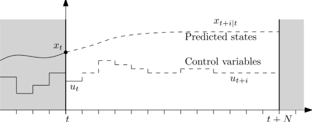
MPC is an optimization-based control technique, where the control inputs are selected based on the current state and predicted state trajectories. Specifically, at each sampling instant, a mathematical model of the system is simulated over a finite horizon and the sequence of control inputs over the horizon is optimized with respect to a performance criterion. The first element of the sequence is then applied to the real plant and a new open-loop optimal control problem is solved at the next sampling instant. Feedback is thus generated into the control scheme. The principle is illustrated in Figure 2.1.

To formulate the open-loop optimal control problem, we consider the follow-ing controlled dynamical system:

˙

x(t)= F(x(t),u(t)) (2.1)

wherex(t)∈_Rnx_{denotes the (di}ff_{erential) states of the system,}_u(t)_∈

Rnu _denotes

the controls representing the actuation in the system, and the system dynamics is determined byF :Rnx×Rnu → Rnx. In the context of control, it is often beneficial

to represent the system (2.1) explicitly at discrete points, i.e.:

xi+1 = f(xi,ui), x0 = x(t0) (2.2)

where we have introduced the simplified notation xi = x(ti) andui = u(ti), and

the controls are assumed to be constant functions between the sampling instants,

(28)

Chapter2. ModelPredictiveControl t t+N ut+i x_t₊_i_|_t Predicted states ut xt Control variables

Figure 2.1: Illustration of the finite-horizon prediction. The notation xt+i|t refers

to the predicted state at time instantt+ibased on information at time instantt.

i.e.:

u(t)=ui, t ∈[ti,ti+1) (2.3)

The state transition mapping f :Rnx×Rnu →Rnxis often approximated, although

it can be represented exactly as: f(xi,ui)= x(ti)+

Z ti+1

ti

F(x(τ),u(ti))dτ (2.4)

By using (2.2), the current statextand a sequence of control variables{ut+k}_kN₌−₀1,

the state trajectory can be predicted over a horizonN as:

           xt+1|t = f(xt,ut) ... xt+N|t = f(xt+N−1|t,ut+N−1) (2.5)

where the notationxt+i|t refers to the predicted states at time instantt+ibased on

information at time instantt. In the following, for notation simplicity, we assume thatt=0 and omit to explicitly denote the dependence of the prediction ont, i.e. we usexi = xt+i|t.

Since the control variables can be manipulated, it is natural to aim at se-lecting them optimally. In this context, we measure optimality by the following performance criterion: V(x,u)=`N(xN)+ N−1 X i=0 `(xi,ui) (2.6)

which takes lower values for favourable states and controls compared to less favourable ones, and where we have introduced the notations x = [xT

0, . . .x

T N]

T

andu = [uT₀, . . .uT_N₋₁]T for the collection of state and control variables over the horizon.

(29)

2.1. StandardMPC

The open-loop optimal control problem, which in the following is referred to as theMPC problem, can then be formulated as:

min x,u V(x,u) (2.7a) s.t. xi+1 = f(xi,ui), i=0, . . . ,N−1 (2.7b) x0 = x(t0) (2.7c) ui ∈ U, i= 0, . . . ,N−1 (2.7d) xi ∈ X, i=0, . . . ,N−1 (2.7e) xN ∈ XN (2.7f)

where the stage constraint setsUandXare assumed to be non-empty and closed, and represent control and state constraints such as e.g. physical limitations and safety restrictions of the system. The terminal constraint setXN is instrumental

to guarantee closed-loop stability [4]. Note that (2) is amultiparametric program with the initial state as the parameter. This, together with the highly structured nature of (2), is often heavily exploited in the design of optimization methods for MPC problems.

Let us now remark on a practically important class of MPC problems, often labeled as linear MPC. In this class, the dynamics are yielded by a linear sys-tem, the cost function is a separable convex quadratic function, and the stage constraint setsXandUand theterminal constraint setXN are polyhedral. This means that the MPC problem takes the form of the following structured QP, which has earned a lot of attention in the literature:

min x,u N−1 X i=0        1 2 " xi ui #T" Qi Si ST_i Ri # " xi ui # + " qi ri #T" xi ui #      + 1 2x T NPxN +qTNxN (2.8a) s.t. xi+1 = Axi+Bui, i=0, . . . ,N−1 (2.8b) x0 = x(t0) (2.8c) C xi+Dui ≤ di, i= 0, . . . ,N−1 (2.8d) DNxN ≤dN (2.8e)

A major challenge in MPC is to solve the underlying optimization problems sufficiently fast. To that end, a variety of customized optimization techniques have emerged to exploit the intrinsic structure of the MPC problems. The struc-ture is mainly stemming from the following two observations.

First, because of the stage-wise structure of the objective function, it is sepa-rable with respect to the time stages and its Hessian isblock-diagonal. Secondly, the constraints are a combination of stage-wise restrictions and dynamic con-straints. This means that variables are only directly affected by other variables

(30)

Chapter2. ModelPredictiveControl

atneighboring time stages. These structures can, as we shall see, be exploited to significantly reduce the memory requirements and computational times for solving (2.7) and (2.8).

2.2 Multi-stage MPC

In this section we provide a brief introduction to multi-stage MPC and formulate the underlying optimization problem; for a more comprehensive description see [62].

To formulate the MPC problem in this case, we consider a discrete-time, constrained system with uncertain parametersθ:

xi+1 = f(xi,ui, θ) (2.9a)

xi ∈ X(θ), ui ∈ U(θ) (2.9b)

To account for the uncertain parameters, we considermdrealizations ofθat each

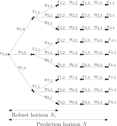
time stage. The predicted state trajectory over a horizonNcan then be described by a scenario tree, as depicted in Figure 2.2, where each branch corresponds to a specific realization of the uncertainty.

We define a scenario as a path from the root node to a leaf node of the sce-nario tree. This means that each scesce-nario corresponds to a unique sequence of realizations of the uncertainty, and accordingly that the number of scenarios is growing exponentially with the length of the MPC horizon, yielding very large MPC problems. It is therefore often proposed to treat the uncertain parameters as constant after a certain period of time. This simplification is motivated by the fact that a new MPC problem is solved at the next sampling instant, implying that an accurate model of the far future is not critical. We denote the time pe-riod where the parameters can change as therobust horizon Nrin contrast to the

prediction horizonN. Accordingly, we consider M= mNr

d scenarios.

Let us consider separate state and control variables for each scenariok, i.e. we introducexk =[xT_k_,₀. . .x_kT_,_N]T ∈Rn¯x, withxk,i ∈Rnxanduk = [uT_k_,₀. . .uT_k_,_N₋₁]T ∈ Rn¯u, withuk,i ∈ Rnu fork = 1, . . . ,M. However, because the uncertainty cannot

be anticipated, control actions are restricted to only depend on historical real-izations of the uncertainty, such that the control variables of the scenarios are coupled at their shared nodes. More specifically, if the uncertainty realizations for scenariok andl are identical up to and including time stagei, their control inputs should be identical up to that time stage, i.e.uk,j =ul,j,∀j=0, . . . ,i. This

restriction is commonly denoted asnon-anticipativity constraints. By considering the following performance criterion for scenariok:

Vk(xk,uk)=ωkV(xk,uk) (2.10)

(31)

2.2. Multi-stageMPC

Figure 2.2: The evolution of the system represented as a scenario tree. In this example,md = 3, Nr = 2 and M = 9. For nodes and branches that are shared

between multiple scenarios, the variable corresponding to the scenario with the lowest index is visualized in the tree.

(32)

whereV is defined in (2.6) andωk denotes the probability of occurrence of

sce-nariok, the multi-stage MPC problem can then be formulated as:

min x,u M X k=1 Vk(xk,uk) (2.11a) s.t. xk,i+1= f(xk,i,uk,i, θk,i), k=1, . . . ,M, i=0, . . . ,N−1 (2.11b) xk,0= x(t0), k =1, . . . ,M (2.11c) xk,i ∈ X, k=1, . . . ,M, i=0, . . . ,N−1 (2.11d) uk,i ∈ U, k =1, . . . ,M, i= 0, . . . ,N−1 (2.11e) xk,N ∈ XN, k= 1, . . . ,M (2.11f) uk,i =ul,i, ifxk,i = xl,i, k,l= 1, . . . ,M, i=0, . . . ,Nr (2.11g)

where we have introduced the notationsx=[xT

1 . . .x T M] T _and_u=_[uT 1 . . .u T M] T_for

the collection of variables over the scenarios, andθk,i denotes thekth realization

ofθat time instanti.

Let us now note that (2.11) is composed of Mordinary MPC problems that are coupled via the non-anticipativity constraints. This observation can, as we shall see in Part II, be exploited in order to design highly parallelizable optimiza-tion methods for (2.11).

2.2.1 Two-stage MPC

A common way of reducing the size of (2.11) is to restrict the scenario tree to only branch in its root node, i.e. to chooseNr =1. The multi-stage MPC problem

is then reduced to atwo-stage MPC problem:

min x,u md X k=1 Vk(xk,uk) (2.12a) s.t. xk,i+1 = f(xk,i,uk,i, θk,i), k=1, . . . ,md, i=0, . . . ,N−1 (2.12b) xk,0= x(t0), k =1, . . . ,md (2.12c) xk,i ∈ X, k =1, . . . ,md, i=0, . . . ,N−1 (2.12d) uk,i ∈ U, k= 1, . . . ,md, i= 0, . . . ,N−1 (2.12e) xk,N ∈ XN, k= 1, . . . ,md (2.12f) uk,0= ul,0, k,l=1, . . . ,md (2.12g)

Note that the only structural difference between the two-stage MPC problem and the multi-stage MPC problem lies in the non-anticipativity constraints. This formulation drastically reduces the number of scenarios, whereas a good perfor-mance can be obtained in practice [63, 64].

(33)

2.3. DistributedMPCvia distributed optimization

However, let us observe the following. The two-stage MPC problem does not model the fact that a new scenario tree, shifted in time, is considered at the next sampling instant. Hence, the second-stage control variables are less restricted compared to the first-stage control variables at the next sampling instant. This means that the controller could end up inrecursive infeasibility. We are, how-ever, not aware of an example where this occurs.

2.3 Distributed MPC via distributed optimization

In this section, we formulate a distributed MPC problem as a separable optimiza-tion problem.

Let us consider a large-scale system that consists ofPsubsystems:

xk,i+1 = fk(xk,i,uk,i), k=1, . . . ,P (2.13)

which are interacting via the followingcoupling constraints:

gi(x1,i,u1,i, . . . ,xP,i,uP,i)=0 (2.14)

where xk,i anduk,i represent state and control variables for subsystemk at time

instant i. Since the subsystems are often sparsly interconnected, the Jacobian matrix ofgi is typically sparse.

By using a performance criterion which is separable in the subsystems, the resulting MPC problem can be formulated as the following separable problem:

min x,u P X k=1 Vk(xk,uk) (2.15a) s.t. xk,i+1 = fk,i(xk,i,uk,i), k= 1, . . . ,P, i=0, . . . ,N−1 (2.15b) gi(x1,i,u1,i, . . . ,xP,i,uP,i)=0, i= 0, . . . ,N−1 (2.15c) xk,0 = xk(t0), k= 1, . . . ,P (2.15d) xk,i ∈ Xk, k =1, . . . ,P, i=0, . . . ,N−1 (2.15e) uk,i ∈ Uk, k= 1, . . . ,P, i=0, . . . ,N−1 (2.15f) xk,N ∈ Xk,N, k= 1, . . . ,P (2.15g)

where the sets Xk and Uk represent restrictions on the subsystem k, and Xk,N

denotes the terminal constraint set of subsystemk. Additionally, we have intro-duced the notations xk = [xT_k_,₀. . .xT_k_,_N]T and uk = [uT_k_,₀. . .uT_k_,_N₋₁]T for the state

and control variables for subsystem k, and the notations x = [xT₁ . . .xT_P]T and u= [uT

1 . . .u

T P]

T _{for the collection of variables over all subproblems.}

Note that (2.15) is composed ofPordinary MPC problems that are coupled via the coupling constraints (2.15c). For geographically distributed systems,

(34)

Coordinator

1

2 P

Figure 2.3: Schematic illustration of the coordinator and the distributed subprob-lems.

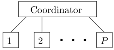
there is often only local knowledge of the subsystems (2.13), and distributed optimization techniques are therefore often desirable. In Part II, we consider Newton strategies for solving (2.15) in a distributed fashion. The problem is then decomposed intoPsubproblems, although in general the resulting methods require a coordinator and can thus be classified as partly distributed as depicted in Figure 2.3.

(35)

Chapter 3 Convex optimization

In this chapter, we recall results and methods from convex optimization which are instrumental for the results in Part II of the thesis.

3.1 Convex sets and functions

In this section we provide a brief introduction to convex sets and functions; for a more detailed description see e.g. [65]

A setS is convexif for any points z1,z2 ∈ S and any scalarθ ∈ [0,1], we

have:

θz1+(1−θ)z2∈ S (3.1)

Thus, the line segment between any two points in a convex set is also in the set. Figure 3.1 illustrates a convex and a non-convex set inR2.

A function f :Rn →Risconvexif dom f is a convex set and for any points

z1,z2∈dom f and any scalarθ∈[0,1], we have:

f (θz1+(1−θ)z2)≤ θf(z1)+(1−θ)f(z2) (3.2)

S1 _S2

Figure 3.1: The setS₁is a convex set whereas the setS₂is a non-convex set.

(36)

Chapter3. Convex optimization

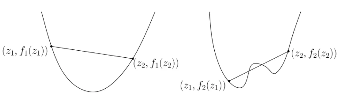
(z1, f1(z1))

(z2, f1(z2))

(z1, f2(z1))

(z2, f2(z2))

Figure 3.2: The function f1 is a convex function whereas the function f2 is a

non-convex function.

Geometrically this means that a function is convex if the line segment between any points (z1, f(z1)) and (z2, f(z2)) lies above or on the graph of f as illustrated

in Figure 3.2.

For differentiable functions, so-called first-order conditions can be estab-lished for the first-order Taylor expansion of convex functions. A diff eren-tiable function f is convex if and only if dom f is convex and for any points z1,z2∈dom f the following inequality holds:

f(z1)≥ f(z2)+∇f(z2)T(z1−z2) (3.3)

This implies that the first-order Taylor expansion of a convex function is a global underestimator of the function. Additionally, we say that a function is strictly convexif (3.3) holds with strict inequality for z1 , z2. Moreover, we say that

a differentiable function f is strongly convex with parameter σ > 0 if for any z1,z2∈dom f it holds that:

f(z1)≥ f(z2)+∇f(z2)T(z1−z2)+

σ

2kz1−z2k

2

(3.4) Observe that strong convexity implies strict convexity but not vice versa.

Assuming that f is twice differentiable, so-called second-order conditions for convexity can be established. A twice differentiable function f is convex if and only if dom f is convex and the Hessian of f is positive semidefinite, i.e.:

∇2f(z) 0 (3.5)

for allz∈dom f. Note that if (3.5) holds with strict inequality f is strictly con-vex, i.e. if dom f is convex and the Hessian of f is positive definite. Similarly, a twice differentiable function f is strongly convex with parameterσ >0 if dom f is convex and it holds that:

∇2f(z)σI (3.6)

for allz∈dom f. Hence, the minimum eigenvalue of∇2_f_{(z) is at least}σ_.

(37)

3.2. Convex optimization problems

Finally, to exemplify the difference between strictly convex functions and strongly convex functions, let us consider the following scalar valued function:

f(z)=ez (3.7)

Note that f is strictly convex since f00(z) >0, although it is not strongly convex since the second derivative can be arbitrary close to zero.

3.2 Convex optimization problems

In this section we provide a brief introduction to convex optimization problems. For a more detailed description see e.g. [65].

Throughout this thesis we consider various forms of the following convex optimization problem:

min

z f(z) (3.8a)

s.t. Az=b (3.8b)

hi(z)≤0, i= 1, . . . ,m (3.8c)

wherez∈_Rn_{is a vector of}_{decision variables,} _f _:

Rn→ Ris a convexobjective

function, A∈_Rp×n_and_b_∈

Rp, and theinequality constraint functions hi :Rn → R, i = 1, . . . ,m are convex. To simplify notations, we use in the following the

vector notation: h(z)=             h1(z) ... hm(z)             (3.9)

A pointz is called feasibleif it satisfies the constraints, i.e. if Az = band h(z) ≤ 0, and strictly feasible if it is feasible and satisfies the inequality con-straints with strict inequality, i.e. if Az = b and h(z) < 0. For notational con-venience, we denote the feasible set asZ = {z : Az = b, h(z) ≤ 0}. The opti-mization problem (3.8) is called feasible if there exists at least one feasible point, and infeasible otherwise. The optimal value of (3.8) is denoted as f?, where we use the convention of letting f? = ∞ for infeasible problems and f? = −∞for problems that are unbounded from below.

A finite value of f? does, however, not guarantee that there exists an optimal solution z? such that the optimal value is attained. To exemplify this, let us consider the following unconstrained problem:

min

z e z

(3.10) In this case, it is clear that f? = 0 although there exists no (bounded) z? such thatez? = _{0. The existence of a bounded} _z? _{such that} _f_(z?₎ = _f? _{is attained is}

(38)

specified in an important theorem due to Weierstrass. Here, we state a simplified version of this theorem:

Proposition 1 Let Z be nonempty and closed, and let f be strongly convex. Then there exists a z?such that:

f(z?)=min

z∈Z f(z) (3.11)

Proof 1 See e.g. [66].

Note that this is a slight modification of Weierstrass’ theorem where we have exchanged lower semi-continuity of f and the weak coercivity of f with respect toZto strong convexity of f. This is a more restrictive requirement since every convex function is also continuous and every strongly convex function is also coercive but not vice versa. In the rest of the thesis, we will assume that there exists a boundedz? such that f(z?)= f?is attained.

If the objective function f is differentiable and a bounded optimal point z? ∈ Zexists, then the optimal point fulfills the following so-called first-order optimality condition:

∇f(z?)T(z−z?)≥ 0, ∀z∈ Z (3.12)

Geometrically this means that if∇f(z?)_, 0, there is no feasible directionz−z? which is also a descent direction in f.

Finally, as a motivation for the next subsection, let us define arelaxationof the problem (3.8). Consider the following problem:

min

z∈ZR

fR(z) (3.13)

We say that (3.13) is a relaxation of (3.8) if fR : Rn → Ris a function such that

fR(z) ≤ f(z), ∀z∈ Z, andZ ⊆ ZR. If we denote the optimal value of (3.13) as

f_R?, we can state the following result for the pair of problems:

Theorem 1 The following properties hold: 1. f_R?≤ f?.

2. If (3.13) is infeasible, then so is (3.8).

3. If (3.13) has an optimal solution z?_R such that z?_R ∈ Zand fR(z?R) = f(z

?

R),

then z?_R is an optimal solution to (3.8) as well.

Proof 2 See [66].

As we shall see, this is an important result since many optimization algorithms seek a solution not to the considered problem but to a relaxation of the considered problem.

(39)

3.2. Convex optimization problems

3.2.1 Lagrangian duality

In many problems, there is a subset of the constraints that makes the problem significantly harder to solve, so-called complicating constraints. The idea in Lagrangian duality is to augment the objective function with the constraints, and it can therefore often serve as a vital tool in the design of optimization methods for problems involving complicating constraints.

Let us denote a subset of the constraints (3.8b) and (3.8c) as: ¯

Az=b¯ (3.14a)

¯

h(z)≤ 0 (3.14b)

where ¯A∈_Rp¯×n_{, ¯}_b_∈

Rp¯for ¯p≤ p, and ¯h:Rn →Rm¯ for ¯m≤ m. Additionally, we

introduce the notationZC

for the feasible set defined by the constraints in (3.8b) and (3.8c) that are not included in (3.14).

By introducing the dual variablesµ ∈ _Rp¯ _and_λ _∈

Rm¯ corresponding to the

constraints (3.14a) and (3.14b) respectively, we define the (partial) Lagrange functionas:

L(z, µ, λ)= f(z)+µT( ¯Az−b)¯ +λTh(z)¯ (3.15) Hence, the Lagrange function is defined by the objective function augmented with a weighted sum of constraint functions. The (negated) Lagrange dual func-tion is then defined as:

d(µ, λ)=−min

z∈ZCL(z, µ, λ) (3.16)

Under some (rather weak) conditions, the Lagrange dual function is diff eren-tiable. This is summarized in the following proposition.

Proposition 2 Assume thath(z)¯ is continuous and convex and that (3.8) is fea-sible. Then the dual function d(µ, λ)is differentiable with gradient:

∇d(µ, λ)= − " _¯ Az?(µ, λ)−b¯ ¯ h(z?(µ, λ)) # (3.17) where z?(µ, λ)= arg minz∈ZCL(z, µ, λ).

Proof 3 See e.g. [67].

We usually restrict the problem data further, and can then obtain a continuously differentiable dual function:

Proposition 3 Assume that h(z)¯ = Cz −d, that (3.8) is feasible and that f is continuous and strongly convex. Then the dual function d(µ, λ)has a Lipschitz continuous gradient.

(40)

Chapter3. Convex optimization Proof 4 See e.g. [68].

One important property of the Lagrange dual function is that it yields a lower bound on the optimal value f?of (3.8). More specifically, for anyµandλ ≥ 0 and any feasible ˜z∈ Z, we have that:

−d(µ, λ)= min z∈ZC f(z)+µT( ¯Az−b)¯ +λTh(z) ≤ f(˜z)+µT( ¯A˜z−b)¯ +λTh(˜z)≤ f(˜z) (3.18)

where the second inequality is stemming from the fact that:

µT

( ¯A˜z−b)¯ +λTh(˜z)≤0 (3.19)

Consequently, the Lagrange dual function is a relaxation of (3.8) wheneverλ≥

0, and (3.16) is then commonly referred to as aLagrangian relaxation. The best possible lower bound−d?that can be obtained from the Lagrange dual function is given by the followingLagrange dual problem:

min

µ,λ d(µ, λ) (3.20a)

s.t. λ≥0 (3.20b)

where we refer to the difference between the optimal value f? and−d? as the optimal duality gap. If the optimal duality gap is zero, i.e. if f? = −d?, we say thatstrong dualityholds. Strong duality is an important property since it implies that the primal solution can be recovered from the dual solution:

Proposition 4 Suppose that strong duality holds and that µ? and λ? solve the Lagrange dual problem. Then, z?is a primal optimal solution if and only if z?is feasible in (3.8) and: z? ∈arg min z∈ZCL(z, µ ?_{, λ}? ) (3.21) Proof 5 See [66].

As we shall see, this is an important result since the Lagrange dual problem and (3.21) often are significantly easier to solve compared to directly solving the primal problem.

There are several so-called constraint qualifications (CQs) to ensure that strong duality holds. In this thesis, we consider the following two commonly used CQs.

Definition 1 The system of constraints describing the feasible region Zis said to satisfy Slater’s constraint qualification if A has full row rank and there exists a point z∈ Zsuch that h(z)< 0.

(41)

3.2. Convex optimization problems Definition 2 The Linear Independence Constraint Qualification (LICQ) is said to be satisfied at a point z∈ Zif the gradients∇hi(z), i=1, . . . ,m together with

AT _{are linearly independent.}

Let us now assume that strong duality holds. Under this assumption, we can conclude that: f(z?)=−d(µ?, λ?)= min z∈ZCL(z, µ ?_{, λ}?₎ = min z∈ZC       f(z)+ µ ?T¯ Az−b¯+ ¯ m X i=1 λ? i h¯i(z)        ≤ f(z?)+ µ?T_¯ Az?−b¯+ ¯ m X i=1 λ? i h¯i(z?) ≤ f(z?) (3.22)

where the first equality is due to strong duality, the second equality follows from the definition of the dual function, and the last inequality holds sincez?is primal feasible, i.e. since ¯Az?−b¯ =0 and ¯h(z?)≤ 0. Accordingly, we can conclude that the inequalities in (3.22) can be replaced by equalities, and hence that:

¯ m X i=1 λ? ih¯i(z?)= 0 (3.23)

Since every term in the sum is non-negative, it follows that:

λ?

i h¯i(z?)= 0, i=1, . . . ,m¯ (3.24)

This condition is referred to ascomplementary slackness, and holds for any pri-mal optipri-mal solutionz?and dual optimal solutionµ?andλ?when strong duality holds.

3.2.2 KKT optimality conditions

It is often of importance to have easily verifiable criteria to check whether a cer-tain point is optimal or not. In this subsection we use the results from Lagrangian duality to develop the classical Karush-Kuhn-Tucker (KKT) conditions.

Let us assume that f andhin (3.8) are differentiable and that all constraints are dualized, i.e. thatZC =

Rn. Now, recall that an optimal pointz? minimizes L(z, µ?, λ?) overz ∈_Rn_{. This means that the gradient of the Lagrange function}

must vanish at the minimizerz?, i.e. at any optimal pointz? the following must hold: ∇f(z?)+ATµ?+ m X i=1 λ? i ∇hi(z?)=0 (3.25) 23

(42)

Additionally, assuming that strong duality holds, we recall that complemen-tary slackness must be satisfied for an optimal primal-dual solutionz? ∈ Z, µ? andλ? ≥ 0. This implies that any pair of primal and dual optimal points must satisfy: ∇f(z?)+ATµ?+∇h(z)λ? =0 (3.26a) Az?−b=0 (3.26b) hi(z?)λ?i =0, i= 1, . . . ,p (3.26c) hi(z?)≤0, i= 1, . . . ,p (3.26d) λ? i ≥0, i= 1, . . . ,p (3.26e)

The conditions (3.26) are called the KKT conditions. Following from the dis-cussion in Section 3.2.1, the KKT conditions are clearly sufficient and necessary conditions for optimality provided that the problem is convex and strong duality holds. However, without strong duality, i.e. without a constraint qualification, the KKT conditions remain only sufficient for convex problems. To exemplify this, let us consider the following convex problem:

min

z z1 (3.27a)

s.t. z2₁+z2 ≤0 (3.27b)

−z2 ≤0 (3.27c)

Note that there is only one feasible point, i.e. z = 0, and Slater’s CQ is hence not satisfied. Additionally, at this point both inequality constraints are active and LICQ is violated. The KKT conditions are:

" 1 0 # + " 0 0 1 −1 # λ= " 0 0 # (3.28a) λ≥0 (3.28b)

which clearly are unsolvable. Hence, this shows a situation in which the KKT conditions are not fulfilled at the optimal solution, and thus demostrates the im-portance of constraint qualifications.

3.3 Dual decomposition

In this section we recall dual decomposition on which some of the results in Part II are based.

(43)

3.3. Dual decomposition

Let us consider the following separable convex optimization problem: min z N X k=1 fk(zk) (3.29a) s.t. N X k=1 Akzk = b (3.29b) zk ∈ Zk, k=1, . . . ,N (3.29c)

wherezk ∈Rnk are vectors of local decision variables, fk : Rnk → Rare convex

functions,Ak ∈Rp×nk, and the setsZk are convex and fulfill a constraint

qualifi-cation such that strong duality holds. Additionally, for notational simplicity, we have introduced the notationz=[zT

1 . . .z

T N]

T _{and use}_Z=_Z

1× · · · × ZN.

Note that the equality constraint (3.29b) acts as a complicating constraint, since it involves all decision variables in contrast to the local constraints (3.29c). To decompose the problem (3.29), we introduce the dual variablesλ∈_Rp

corre-sponding to the complicating constraint (3.29b) and define the Lagrange function as: L(z, λ)= N X k=1 fk(zk)+λT        N X k=1 Akzk −b        (3.30)

where we note thatL(z, λ) is separable inz, i.e. it can be expressed as:

L(z, λ)= N X k=1 Lk(zk, λ) (3.31) where: Lk(zk, λ)= fk(zk)+λ T Akzk − 1 Nb ! (3.32) The Lagrange dual functiond(λ) = −minz∈ZL(z, λ) can thus be evaluated in parallel as: d(λ)=− N X k=1 min zk∈Zk Lk(zk, λ) (3.33)

where we have interchanged the order of the minimization and summation. As-suming that the Lagrange dual function is differentiable, according to Proposition 2, its gradient can be calculated as:

∇d(λ)=− N X

k=1

Akz?k(λ)+b (3.34)

wherez?_k(λ) = arg minzk∈ZkLk(zk, λ) can be calculated in parallel. As a result,

the Lagrange dual problem can be decomposed and solved in a parallel fashion using e.g. gradient-based optimization methods.

(44)

zk _zk_{+ ∆}_z

z

r(zk₎

z⋆

r(zk_{+ ∆}_z₎

Figure 3.3: Illustration of Newton’s method.

3.4 Optimization methods

In this section, we recall the optimization methods on which the results in Part II are based.

3.4.1 Newton’s method

The essence of many optimization routines is to find a solution to a nonlinear system of equations, i.e. the problem of findingz? ∈_Rn_{such that:}

r(z?)=0 (3.35)

wherer:_Rn _→

Rnis a smooth vector valued function, i.e.:

r(z)=             r1(z) ... rn(z)             (3.36)

In practice, one of the most consistently efficient methods for finding a solu-tionz? to a system of the form (3.35) is Newton’s method. In Newton’s method a solution is searched by iteratively linearizingrand performing steps that fulfill the linearizations as illustrated in Figure 3.3. The core of the method is thus to solve the following so-calledNewton systemin order to find theNewton direction

∆z:

∂r(zk₎

∂z ∆z=−r(z

k

) (3.37)

The variables are then updated in the direction of the Newton direction according to:

zk+1 =zk +t∆z (3.38)

(45)

3.4. Optimization methods

wheret ∈(0,1] is an appropriately chosenstep sizeto enforce convergence and speed of the iteration.

Provided that there exists a solutionz? to the system (3.35) and that ∂r_∂(z_zk) is full rank, Newton’s method provides a contractive iteration for findingz? if we provide an initial guess sufficiently close toz?. Here, we omit to further specify whatclose enoughmeans, and only state that it depends on how nonlinearr is, for details see e.g. [69].

To exemplify the usefulness of Newton’s method in optimization, let us con-sider the following unconstrained convex problem:

min

z f(z) (3.39)

Due to the absence of constraints, the first-order optimality condition simplifies to:

∇f(z?)= 0 (3.40)

Hence, the solutionz?to (3.39) is also solving the nonlinear system of equations (3.40). Applying Newton’s method on the system (3.40) results in the following Newton system:

∇2f(zk)∆z=−∇f(zk) (3.41)

A useful interpretation of this system is that the Newton direction is the mini-mizer of a quadratic model of f around the current point zk. Specifically, ∆zis the solution to the following unconstrained Quadratic Program (QP):

min z f(z k )+∇f(zk)Tz+ 1 2z T_∇2_f_(zk )z (3.42)

This interpretation often provides insights into when Newton’s method may be successful in solving an unconstrained optimization problem and when it may fail. In cases where f can only be inaccurately modeled by a quadratic function atzk_{, the selection of the step size}_t_{is instrumental.}

In the context of unconstrained optimization, the step size t is commonly chosen by abacktracking line-search. This means that the step size is initialized at a relatively large value and iteratively reduced until a condition measuring progress is fulfilled. In this thesis, we use theArmijo conditionin the backtrack-ing line-search. This means that for every search direction∆z, we initialize the step size att=1 and backtrack according to:

t :=βt (3.43)

until the Armijo condition is fulfilled, i.e. until:

f(zk+t∆z)≤ f(zk)+αt∇f(zk)T∆z (3.44)

(46)

f(zk₊_t_∆_z₎

f(zk_{) +}_tα_∇_f₍_zk₎T_∆_z

f(zk_{) +}_t_∇_f₍_zk₎T_∆_z t

Figure 3.4: Illustration of the Armijo condition.

for some constantsα, β ∈ (0,1). To gain some insights into the choice of the parametersαandβ, let us recall (3.3) and note that if f is nonlinear (3.44) would never be fulfilled forα = 1, since a linearization is a global underestimator of a convex function. By reducingα, however, the slope is reduced and the linear function will always intersect f. Evidently, for convex problems it is always possible to find a step sizet ∈ (0,1] such that (34) is fulfilled. Following from the discussion, we also note that large values ofαandβ correspond to a crude line-search whereas small values correspond to a careful search. An illustration of the Armijo condition is provided in Figure 3.4.

Note that for a twice differentiable convex function f,∇2f(zk) is only positive semidefinite, i.e. there could be directions in which f lacks curvature. Such cases are problematic since a rank deficient ∇2_f_{(z) leads to an inconsistent Newton}

system. This problem is in general addressed by adding a regularization matrix F ∈_Sn

+to∇2f(zk) to ensure that:

∇2f(zk)+F 0 (3.45)

One common choice is the so-calledLevenberg-Marquardt regularizationwith F =δI.

Algorithm 1Newton’s method for unconstrained minimization

1: fork≥ 0 do

2: CalculateF

3: Solve (∇2f(zk₎+_F)∆_z= _−∇_f_(zk₎

4: Perform line-search to find an appropriatet

5: zk+1 =zk+t∆z

6: end for

A basic Newton method for unconstrained convex minimization is provided in Algorithm 1. The computational bottleneck in Newton’s method typically lies in solving the Newton system. This means that any structure that can enhance its solution should be exploited.

(47)

3.4. Optimization methods

If the function f lacks enough differentiability or if the Newton system de-spite structure exploitation is too costly to solve, ∇2f(zk) is typically approxi-mated in the Newton system by a matrix that is cheaper to compute. The result-ing method is then referred to as aquasi-Newton method.

3.4.2 Primal-dual interior point methods

Due to their robustness and consistent practical performance, interior point meth-ods are often the preferred choice to solve problems of the form (3.8). In this subsection, we recall the basics ofprimal-dual interior point methods.

In primal-dual interior point methods, Newton’s method is used to solve a modified version of the KKT conditions. To motivate the modification, we recall that Newton’s method offers a practically efficient way of solving a system of smooth nonlinear equations. This means that the non-smooth complementary relationship betweenh(z?) andλ?in the KKT conditions is problematic. Thus, to smoothen the KKT conditions, the complementary slackness condition is relaxed as:

hi(z)λi =τ, i=1, . . . ,p (3.46)

whereτ≥ 0 is referred to as thebarrier parameter.

Additionally, to facilitate the enforcing of the inequality constraints, slack variables s ∈ _Rp _{are typically introduced, and the inequality constraints are}

re-formulated as:

h(z)+s=0 (3.47a)

s≥0 (3.47b)

The resultinginterior point KKT conditionsare given by:

0= ∇L(z,s, µ, λ)= ∇f(z)+ATµ+∇h(z)λ (3.48a)

0= Az−b (3.48b)

0= h(z)+ s (3.48c)

0= Sλ−τ1 (3.48d)

λ≥0, s≥ 0 (3.48e)

where we have introduced the notation S = diag(s) and 1 ∈ _Rp represents a vector of ones. Note that by decreasingτ, (3.48) can be an arbitrary good ap-proximation of the KKT conditions.

By fixingτand applying Newton’s method on the system (3.48a)-(3.48d) in the variablesz, µ, λand swe obtain the so-calledinterior-point KKT systemor

(48)

Chapter3. Convex optimization primal-dual system:                ∇2 zzL k AT ∇h(zk) A ∇h(zk₎T _I Sk Λk                               ∆z ∆µ ∆λ ∆s                =−                ∇zLk Azk₋_b h(zk₎+ _sk Λk sk−τ1                (3.49)

where we have introduced the notationsLk = L(zk,sk, µk, λk) andΛk =diag(λk). The primal-dual variables are then updated according to:

zk+1 =zk +t∆z (3.50a) sk+1 = sk+t∆s (3.50b) µk+1 ₌_µk₊ t∆µ (3.50c) λk+1 ₌_λk ₊ t∆λ (3.50d)

wheret ∈ (0,1] is chosen to enforce sk+1 > _{0 and} λk+1 > _{0. A basic}

primal-dual interior point method is summarized in Algorithm 2, whererk denotes the coefficient vector of (3.49) and >0 serves as a tuning parameter. State-of-the-art primal-dual interior point methods are, however, somewhat more subtle [69].

Algorithm 2Primal-dual interior point method

1: fork≥ 0 do

2: Solve interior point KKT system

3: Find appropriate step sizet

4: Update variables

5: ifkrkk ≤then

6: τ:= ατ

7: end if

8: end for

The computational bottleneck in any modern interior point method lies in the solution of the interior point KKT system, which motivates the development of efficient techniques for factorizing its coefficient matrix. Finally, we recall two reformulations of (3.49) that are commonly used to reduce the computational cost of its solution.

By eliminating ∆s and ∆λ using the bottom two block rows of (3.49), the so-calledaugmented systemis obtained:

" Φk AT A # " ∆z ∆µ # = − " rk_d Azk₋_b # (3.51) where we have introduced:

Φk ₌_∇2_Lk ₊_∇

h(zk)T(Sk)−1Λk∇h(zk) (3.52a)

rk_d =∇Lk +ATµk+∇h(zk)T(Sk)−1Λkh(zk)+ sk (3.52b)

Structure exploiting optimization methods for model predictive control