This is a repository copy of
Non-linear system identification of solvent-based
post-combustion CO2 capture process
.
White Rose Research Online URL for this paper:
http://eprints.whiterose.ac.uk/138999/
Version: Accepted Version
Article:
Akinola, T.E., Oko, E., Gu, Y. et al. (2 more authors) (2019) Non-linear system identification
of solvent-based post-combustion CO2 capture process. Fuel, 239. pp. 1213-1223. ISSN
0016-2361
https://doi.org/10.1016/j.fuel.2018.11.097
Article available under the terms of the CC-BY-NC-ND licence
(https://creativecommons.org/licenses/by-nc-nd/4.0/).
[email protected] https://eprints.whiterose.ac.uk/ Reuse
This article is distributed under the terms of the Creative Commons Attribution-NonCommercial-NoDerivs (CC BY-NC-ND) licence. This licence only allows you to download this work and share it with others as long as you credit the authors, but you can’t change the article in any way or use it commercially. More
information and the full terms of the licence here: https://creativecommons.org/licenses/ Takedown
If you consider content in White Rose Research Online to be in breach of UK law, please notify us by
1
Non-linear system identification of solvent-based post-combustion CO2 capture
process
Toluleke E Akinolaa, Eni Okoa, Yuanlin Gub, Hua-Liang Weib, Meihong Wang a* a Department of Chemical and Biological Engineering, University of Sheffield, Sheffield. S1 3JD b Department of Automatic Control and Systems Engineering, University of Sheffield, Sheffield. S1 3JD
a* Corresponding Author. Tel.: +44 114 222 7160. E-mail address: [email protected]
Abstract
Solvent-based post combustion capture (PCC) is a well-developed technology for CO2 capture
from power plants and industry. A reliable model that captures the dynamics of the solvent-based capture process is essential to implement suitable control design. Typically, first principle models are used, however they usually require comprehensive knowledge and deep understanding of the process. System identification approach is adopted to obtain a model that accurately describes the dynamics between key variables in the process. The nonlinear auto-regressive with exogenous (NARX) inputs model is employed to represent the relationship between the input variables and output variables as two Multiple-Input Single-Output (MISO) sub-models. The forward regression with orthogonal least squares (FROLS) algorithm is implemented to select an accurate model structure that best describes the dynamics within the process. The prediction performance of the identified NARX models is promising and shows that the models capture the underlying dynamics of the CO2 capture
process.
Keywords: Solvent-based post-combustion capture; chemical absorption; System
Identification; NARX; FROLS-ERR
Highlights
First principle dynamic model for solvent-based carbon capture process used to generate data
Solvent-based carbon capture process exhibits a highly nonlinear behaviour
System Identification of solvent-based CO2 capture process using NARX model Significant model term selection using the FROLS-ERR algorithm
Developed NARX model accurately predicts CO2 concentration at absorber outlet and
CO2 lean loading
2
Abbreviations
BIC - Bayesian Information Criterion
CCL - CO2 Capture level
CCS - Carbon Capture and Storage
ERR - Error Reduction Ratio
FROLS - Forward Regression with Orthogonal Least Squares
LL - Lean loading
MIMO - Multiple Input Multiple Output
MISO - Multiple Input Single Output
MP - Mass percentage
MPO - Multi step-ahead Prediction Output
MSE - Mean Square Error
NARX - Nonlinear Auto-regressive with exogenous inputs
NARMAX - Nonlinear Auto-regressive moving average with exogenous inputs
OSA - One-Step Ahead Prediction
PCC - Post Combustion Capture
SISO - Single Input Single Output
Nomenclature
- Dictionary
- Flue gas flowrate at the absorber inlet, kg/s - Treated gas flowrate at the absorber outlet, kg/s - CO2 mass fraction at the absorber inlet
- CO2 mass fraction at the absorber outlet
- Time delay
- Maximum lag in the input - Maximum lag in the output - Response Vector
- Regressors Vector
- Parameter Estimate - Parameter Vector - Number of terms
y1 - CO2 mass percentage at the absorber gas outlet (measured output)
y2 - CO2 lean loading (measured output)
u1 - Flue gas flowrate (measured input)
u2 - Lean MEA flowrate (measured input)
3
1 Introduction
1.1 Background
The utilisation of fossil fuels, particularly coal, for electricity generation is recognised as the single largest source of greenhouse gas emissions[1]. CO2 is the largest anthropogenic greenhouse gas
accounting for about three quarters of the global greenhouse gas emitted to the atmosphere[2]. This has resulted in a steady rise in the global average temperature and brought awareness among scientific communities to tackle issues rising from greenhouse gas (GHG) emissions.
Carbon capture and Storage (CCS) is acknowledged to play a major role in the reduction of CO2
emission from fossil fuel fired power plants. Amongst various CCS technologies, the utilisation of solvent-based post-combustion capture (PCC) process to treat fuel gas from coal fired plant has gained much attention[3]. This is attributed to its suitability to be retrofitted into an existing power plant and its capacity to treat flue gas with low CO2 partial pressure, giving the solvent-based PCC
an edge over other carbon capture technologies[1]. As a result, there has been notable progress in the solvent-based PCC technology development, which has made it the first and only commercial technology that is operational for large-scale coal-fired power plants. Some completed CCS projects include SaskPower Boundary Dam Carbon Capture and Petra Nova Carbon Capture Project[4]. Stringent environmental legislations around the world to reduce CO2 emissions have prompted the
need to deploy new energy sources such as nuclear and renewable energy. This will bring a significant shift in the dominant role of fossil fuel, especially coal, in the energy system and the need for flexible operation of coal fired power plants[5]. The flexible operation of a coal-fired power plant involves the variation of power plant load in accordance to the volatile electricity demand and prices[6]. This result in the fluctuation of the flue gas flowrate and composition to the absorber, as well as steam provided to the reboiler for solvent regeneration, which affects the operation of the capture plant. Thus, the flexible operation of the solvent-based PCC plant (i.e. variation of the capture rate in accordance with electricity demand) is important to cope with the coal-fired power plant operation. Investigation of the capture plant response to disturbances during various flexible operation modes such as start-up, shutdown and load following has gain much attention as well as the need to develop a suitable control strategy for the capture plant to handle these disturbances. 1.2 Literature Review
An accurate and reliable dynamic model is necessary to carry out a comprehensive study on the solvent-based CO2 capture process. Many studies on dynamic modelling of a solvent-based PCC
were carried out on first principle (i.e. mechanistic) models[1,7–12]. Challenges with high computational time when developing a detailed solvent-based PCC model especially when integrated with coal fired power plant and its high level of complexity makes it difficult to implement relevant process control strategies. Thus, simplification of the mechanistic model is required to
4
reduce the computational time for simulation[13,14]. This has significantly motivated the use of data driven modelling approach and system identification techniques, to represent the solvent-based PCC model. This involves constructing a suitable model that best describes the relationship between the process input and output variables.
In the past, most studies have represented the capture process as a linear model[15–20]. It should be noted that the capture process exhibits highly nonlinear behaviour[21]. The linear model is an approximation of the actual model, which tend to deviate from the actual model when large substantial changes in the input variables enter the carbon capture process[17], especially during flexible operation. Thus, a nonlinear model is essential to capture the actual dynamics within the carbon capture process. Only a few studies have applied non-linear modelling techniques such as neural networks[22–24] and non-linear autoregressive with exogenous input (NARX) model[21] to analyse the CO2 capture process.
The key steps of system identification include data collection, model structure detection, and model validation[25]. Various studies on system Identification of nonlinear systems have focused on different classes of system, which included volterra series model[26–28], Hammerstein model, Wiener model, Hammerstein-Wiener model[29] and NARMAX model[30,31]. Amongst these classes of nonlinear models, NARMAX model is one of the commonly used representations suitable for a large range of nonlinear systems[30,31]. The key task in system identification using NARMAX and related models centres on model structure detection. The well-known forward regression with orthogonal least squares (FROLS) algorithm has proven to be one of the most efficient approach for nonlinear model structure determination[30,32–34] for the NARMAX model. The FROLS algorithm selects the important model terms one by one, in a stepwise manner, based on their significance, which is measured using a simple but useful index called the error reduction ratio (ERR).
1.3 Aim and Objectives
This paper aims to introduce a data- driven dynamic modelling approach for the solvent-based PCC plant. In this study, the solvent-based CO2 capture process is represented as NARX models (a
special form of NARMAX model). The FROLS algorithm is used to find a most parsimonious (with least parameters) model to represent the relationship between the input variables (flue gas flowrate, lean MEA flowrate and reboiler temperature) and output variables (CO2 concentration in wt% and
CO2 lean loading).
1.4 Novelty and Structure of Paper
A key novelty of this study is that for the first time, the FROLS algorithm to develop a transparent NARX model that captures the relationship between the input variables and output variables in the carbon capture process. This algorithm enabled us to identify and rank key model terms that contribute to the response variable based on ERR and remove model terms that least contribute to
5
the system output. The FROLS-ERR algorithm has been extensively used in the literature as an effective system identification technique for various systems[35–38]. To our knowledge, the advantages and potentials of nonlinear system identification techniques, especially dynamic NARMAX models identification with the FROLS-ERR algorithm, have not been well explored for PCC processes.
The paper is structured as follows. Section 2 gives a description of the solvent-based PCC process. The system identification approach using FROLS-ERR algorithm is described in Section 3. Data collection and model identification are presented in Section 4, while Section 5 demonstrates the model performance and discusses the results obtained, statistical analysis as well as the step response analysis. Section 6 provides a brief but useful conclusion and future research consideration.
2 Solvent-based PCC Description
2.1 Solvent-based PCC Process
The solvent-based PCC process mainly consists of absorber and stripper with an aqueous mono-ethanolamine solution (MEA) as a chemical solvent. The schematic diagram is shown in Fig 1. The absorber typically receives flue gas from the power plants, which flows in from the bottom. The lean solvent is introduced from the top of the absorber and flows counter-currently to strip out CO2 from
the flue gas. Rich CO2 solvent exits the absorber bottom with the aid of a pump through a heat
exchanger into the regenerator while the treated gas leaves the absorber top into the atmosphere. In the regenerator, CO2 is stripped using heat input from steam extracted from power plants and
exits from the top of the regenerator through a condenser to a compression train, where CO2 gas is
compressed and transported via a pipeline for either enhanced oil/gas recovery and, underground storage or various CO2 utilisation[7]. The regenerated solvent is recycled to the absorber as it flows
from the bottom of the regeneration bottom, through the heat exchanger for energy consumption efficiency and water make-up tank to maintain a constant concentration of water. Insights gained from previous studies on the CO2 capture process was vital in identifying key process variables that
are sensitive to the dynamic performance of the capture plant for flexible operation mode[7]. 2.2 Selection of Input and Output Variables
In various studies, which includes system identification of the solvent-based capture process, the input and output variables selection were based on the control objectives of the capture process. These objectives are centred on environmental and economic (operational) targets[18].
Key parameters that are sensitive to the control objectives are CO2 capture level and regeneration
efficiency. The CO2 capture level (CCL) measures the amount of CO2 captured from the capture
6 Fig 1 Solvent-based PCC process[7]
CCL (1)
where, , , , are CO2 mass fraction at the absorber gas outlet, flue gas
flowrate at the absorber gas outlet, CO2 mass fraction at the absorber gas inlet and flue gas flowrate
at the absorber gas inlet respectively. Thus, the key variable that is sensitive to the CO2 capture level
is the CO2 mass fraction at the absorber gas outlet ( ), which can be represented as CO2 mass
percentage (CO2 -MP). The regeneration efficiency, which accounts for the bulk of the energy
utilisation, is a measure of energy utilised in the regenerator of the capture process. It is acknowledged that the reboiler consumes the most energy and thus dictates the operational cost of the capture process. As stated earlier, steam is extracted from power plants as heat input to the reboiler. The CO2 lean loading (CO2-LL) at the lean MEA stream to the absorber is a key process
variable that is sensitive to the energy efficiency of the CO2 capture process. Thus, CO2–MP and
CO2-LL were selected as the Output variables.
Selection of the input variables was based on key variables (manipulated and disturbance variables) that have significant effect the output variables. Key input variables selected for this study includes flue gas flowrate, lean solvent flowrate and reboiler temperature. Unlike most studies, which used the reboiler duty as an input variable, the reboiler temperature was selected for this study. This is based on study carried out by Lawal et al.[8], in which the reboiler temperature controls the amount of stream drawn off the power plant for regeneration. Thus, the solvent based PCC process was represented as a 3-input and 2-output model.
7
3 NARX Model
The multivariable Nonlinear Auto-Regressive with eXogenous (NARX) input model, which is a special form of Nonlinear Auto-Regressive Moving Average with eXogenous inputs (NARMAX) model[30,31], is adopted to represent the solvent –based PCC process. The NARX model of Multiple-Input and Single-Output (MISO) systems is described as:
(2)
where is the number of external input signals; , , and , with and are measured system output, input and unmeasurable noise sequences, respectively; and are the maximum lags in the output and input; represents a nonlinear function, which is generally unknown but can be approximated using various types of nonlinear forms. Polynomial expansion of is most commonly used due to its good properties, which include transparency and easy interpretation of the model[30].
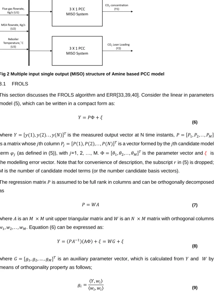
The solvent-based CO2 capture process considered in the present study is a typical MIMO system,
involving three inputs (namely, flue gas flowrate, lean MEA flowrate and reboiler temperature) and two outputs (CO2-MP and CO2-LL). The MIMO system can be represented as two MISO
sub-systems, each of which can be represented using the NARX model (2) as:
(3) (4)
where =3, = flue gas flowrate (kg/s), = Lean MEA flowrate (kg/s), = Reboiler temperature, and and are unmeasurable noise sequences. A graphical illustration of the MISO sub-systems is shown in Fig 2. Each MISO model can be re-arranged into a linear-in-the-parameters form as [39]:
(5)
where , , and , with , are the response signal (output),
regressors, model parameter and number of model terms. Note that each is built using lagged
input and lagged output variables, such as , etc. Further
details can be found in [39]. The forward regression with orthogonal algorithm (FROLS) is used to select significant model terms for each MISO sub-system.
8
Fig 2 Multiple input single output (MISO) structure of Amine based PCC model
3.1 FROLS
This section discusses the FROLS algorithm and ERR[33,39,40]. Consider the linear in parameters model (5), which can be written in a compact form as:
(6)
where is the measured output vector at N time instants,
is a matrix whose th column is a vector formed by the th candidate model
term (as defined in (5)), with =1, 2, …, M. is the parameter vector and is the modelling error vector. Note that for convenience of description, the subscript in (5) is dropped; M is the number of candidate model terms (or the number candidate basis vectors).
The regression matrix is assumed to be full rank in columns and can be orthogonally decomposed as
(7)
where is an unit upper triangular matrix and is an matrix with orthogonal columns . Equation (6) can be expressed as:
A
(8)
where is an auxiliary parameter vector, which is calculated from and by
means of orthogonality property as follows;
(9)
9
with =1, 2, …, M .The parameter vector is related by the equation A . The error reduction ratio (ERR), which provides an effective means for seeking in a subset of significant model term, is calculated as
(10)
The significant model terms are selected in a forward-regression pattern. Details on FROLS algorithm procedure for model structure selection can be found in [30,33,39,40].
4 Data Collection and Model Identification
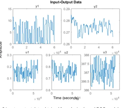
This research obtained dynamic operational data from a dynamically modelled amine- based PCC plant by Lawal et al.[1] using gPROMS and dynamically validated by Biliyok et al.[10]. The simulated data were generated from the model where the time interval for each sample was 60s. All three input variables were simultaneously perturbed for the MISO system representation of the Capture process. Data acquired from the simulation is shown in Fig 3.
Fig 3 Input – output data obtained from Amine based PCC model developed in gPROMS; u1: flue gas flowrate; u2 = Lean MEA flowrate; u3 = reboiler temperature; y1: CO2 concentration in wt% at the absorber gas outlet; y2 = CO2 lean loading (LL) at the lean solvent stream to the absorber.
Data were carefully observed and outliers were removed. Rigorous pre-treatment was not performed to avoid losing some nonlinear dynamics of the system[41]. The whole data were split into estimation data (75%) and validation (test) data (25%). The estimation (training) data were used for model construction, whereas the test data were used to test the model performance in predicting the CO2
10
(LL) at the lean solvent stream to the absorber, (y2). The Input variables used for this model
development are flue gas flowrate (u1), lean MEA flowrate (u2) and reboiler temperature (u3).
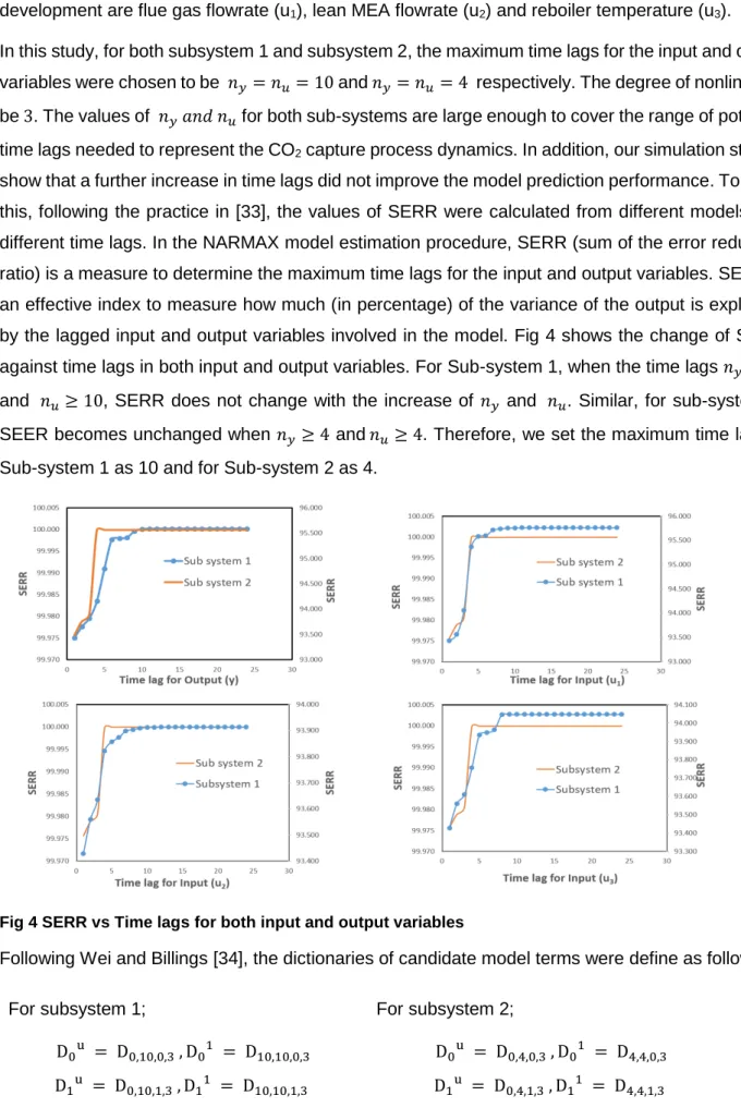
In this study, for both subsystem 1 and subsystem 2, the maximum time lags for the input and output
variables were chosen to be and respectively. The degree of nonlinearity
be . The values of for both sub-systems are large enough to cover the range of potential time lags needed to represent the CO2 capture process dynamics. In addition, our simulation studies
show that a further increase in time lags did not improve the model prediction performance. To show this, following the practice in [33], the values of SERR were calculated from different models with different time lags. In the NARMAX model estimation procedure, SERR (sum of the error reduction ratio) is a measure to determine the maximum time lags for the input and output variables. SERR is an effective index to measure how much (in percentage) of the variance of the output is explained by the lagged input and output variables involved in the model. Fig 4 shows the change of SERR against time lags in both input and output variables. For Sub-system 1, when the time lags
and , SERR does not change with the increase of and . Similar, for sub-system 2,
SEER becomes unchanged when and . Therefore, we set the maximum time lag for
Sub-system 1 as 10 and for Sub-system 2 as 4.
Fig 4 SERR vs Time lags for both input and output variables
Following Wei and Billings [34], the dictionaries of candidate model terms were define as follows:
For subsystem 1; For subsystem 2;
D D D D
D D D D
D D D D
11 where
D
.
A model term dictionary D is a set consisting of a great number of model building blocks (i.e., candidate model terms)[34]. Here, the two dictionaries D and D only contain candidate model terms formed by all input variables alone (i.e., and their lagged versions such as
, etc.) but do not include autoregressive model terms such as
with = 0 and 1 respectively. The other two dictionaries, D and D , however, contain candidate model terms formed by using all the input variables and all the lagged input and output variables. The main purpose that we separately treat these two group of model (with and without autoregressive variables) is to test whether feedback signals from the system outputs play an
obviously important role in explaining the system the system’s inherent dynamics.
Using the above 4 dictionaries, a total of 4 models, different model structures, were identified for each sub-system. The model terms were ranked in accordance with their level of significance (measured by ERR index) to the response variable in each sub-model.
The determination of model length (the number of model terms) is important for dynamic modelling and various model selection criteria have been proposed in the literature. In this
study, the Bayesian information criterion (BIC) is used to determine the number of model terms[42].
ln
(11)
where is the number of samples in the training data set, is the effective number of model terms, is the mean square error associated with the -terms model. BIC is commonly used to avoid over-fitting through the penalty factor ln . The minimum BIC (n) is adopted as the basis for selecting the model length. Thus, the FROLS algorithm stops its iteration at minimum BIC. Each model identified from the different model term dictionaries were compared based on One-step ahead (OSA) predictions and multi-step (10) ahead predicted outputs (MPO). The models that best predict the system outputs were selected based on the MPO performance criterion.
5 Performance Evaluation
5.1 Sub-model 1
Sub-model 1 represents a MISO system to predict the concentration of CO2 in wt% at the absorber
12
candidate dictionary (D D D D ) using FROLS algorithm along with the parameter estimates and BIC. It can deduced from the sum of error reduction ratio (SERR), that the list of model terms selected from dictionaries D gives the best explanation (99.90%) of the response variable variation compared to the identified model developed from other dictionaries (see Table 4) .
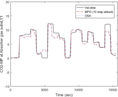
Furthermore, comparisons of the identified models obtained from the different model dictionaries were carried out to assess the predictive ability of the models. Each of the models was applied to the test data for concentration of CO2 in wt% at absorber gas outlet. The associated one-step ahead
predictions and multi-step (10) ahead predicted outputs are calculated and shown in Figs. 5-8, where the solid line represents the original measurements and the dashed blue and red lines are for the one-step ahead prediction and multi-step (10) ahead predicted output, respectively.
As shown in Fig 5 and Fig 7, models M (see Table 1) and model M (see Table 3) gave similar MPO and OSA performance, this is because these models only use exogenous inputs (u(t-1),…,ur (t-1),…,ur(t-n)) and do not use any autoregressive model terms (y(t-1),….,y(t-n)). For models that only
use exogenous inputs (without using autoregressive terms), their MPO and OSA predictions are always the same. Models M and M (see Table 2 and Table 3 respectively), however, involve both the autoregressive variables and the exogenous input variables. Comparing Figs 5-8, it can be seen that model M gave the best prediction performance (Fig 8), indicating that M contains the appropriate model terms that capture the dynamics of the system. For M , there was disparity between the MPO and OSA prediction performances, this is because M does not contain the most appropriate model terms that can well capture the system dynamics. For such a deficient model, its MPO performance will usually deteriorates because the accumulative error can be significantly augmented through an iterative computation procedure when updating the system output values. The OSA performance of such a deficient model, however, normally does not suffer from any error accumulation and propagation. The discrepancy between MPO and OSA shown in Fig 6 (formally Fig 5) is mainly caused by the error propagation and augmentation due to the deficiency of the model. MPO is often used to test the validity of a dynamic model that cannot be easily revealed by OSA.
The variance accounted for (VAF), also called the prediction efficiency (PE), of the identified models are shown in Table 5. VAF (and PE) is calculated as:
VAF var var (12)
where is the measured output of the test data and is the one-step ahead prediction/ multi step-ahead prediction output. Among the 4 models, M M M M (obtained based upon
13
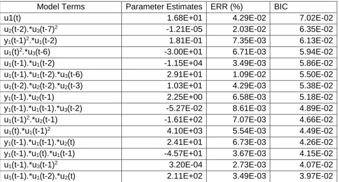
the 4 dictionaries,D D D D ), It can be seen from Table 5 that model M gave the best performance compared to the other 3 models with a prediction efficiency of 98.93% and 98.55% in terms of OSA and MPO respectively (see Fig.8). This indicates that the underlying dynamics between the inputs and the output (concentration of CO2 in wt% at the absorber gas outlet) is
captured by model M [23]. Thus, model M was selected to represent sub-system 1. From Table 4, the system model can be written as:
y t y t u t y t u t
u t u t u t (13)
Table 1 Identified model ( ) structures from for sub-model 1 using FROLS algorithm
Model Terms Parameter Estimates ERR (%) BIC
u1(t-1)2 1.08E+04 8.70E+01 4.04E+00
u1(t-1).*u2(t-1)2 -6.81E+02 3.97E+00 2.84E+00
u1(t-1)3 -5.85E+03 1.47E+00 2.40E+00
u1(t-1)2.*u3(t-10) -2.61E+01 3.55E-01 2.31E+00
u1(t-10)2 -2.65E+02 1.37E-01 2.28E+00
u1(t-10)2.*u2(t-1) 1.35E+02 8.97E-02 2.27E+00
u2(t-1)2.*u2(t-10) -8.58E+00 1.04E-01 2.26E+00
u1(t-1)2.*u2(t-1) 3.01E+03 2.16E-01 2.21E+00
u2(t-1)3 4.42E+01 6.92E-01 2.00E+00
u1(t-1)2.*u1(t-10) -1.49E+02 8.13E-02 1.98E+00
u1(t-10)2.*u2(t-10) 2.18E+02 4.96E-02 1.98E+00
Fig 5 A comparison of the model predictions (OSA and MPO) and measurements over the test data for sub-system 1 using model M (Table 1).
14
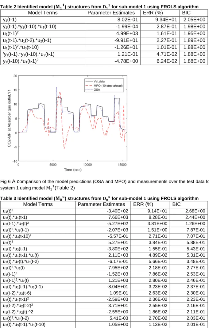
Table 2 Identified model ( ) structures from for sub-model 1 using FROLS algorithm
Model Terms Parameter Estimates ERR (%) BIC
y1(t-1) 8.02E-01 9.34E+01 2.05E+00
y1(t-1).*y1(t-10).*u3(t-10) -1.99E-04 2.87E-01 1.98E+00
u1(t-1)2 4.99E+03 1.61E-01 1.95E+00
u1(t-1).*u1(t-2).*u2(t-1) -9.91E+01 2.27E-01 1.89E+00
u1(t-1)2.*u3(t-10) -1.26E+01 1.01E-01 1.88E+00
'y1(t-1).*y1(t-10).*u2(t-1) 1.21E-01 4.71E-02 1.88E+00
y1(t-10).*u1(t-1)2 -4.78E+00 6.24E-02 1.88E+00
Fig 6 A comparison of the model predictions (OSA and MPO) and measurements over the test data for sub-system 1 using model M (Table 2)
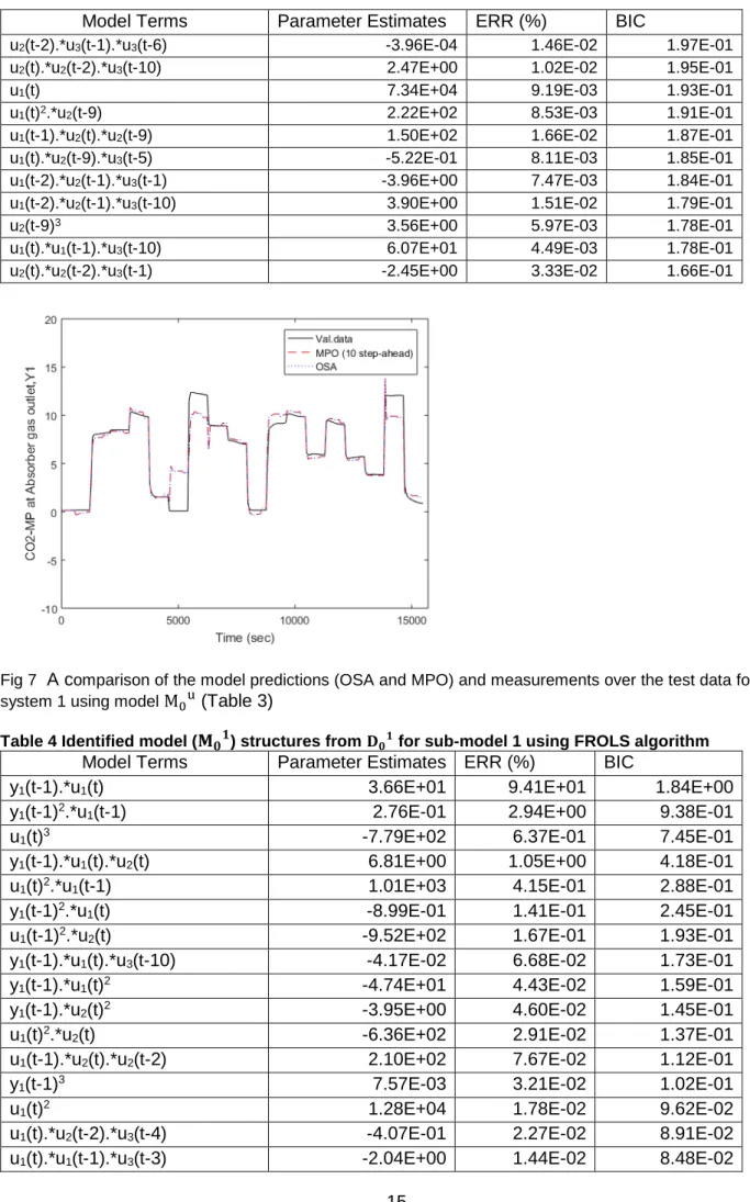
Table 3 Identified model ( ) structures from for sub-model 1 using FROLS algorithm
Model Terms Parameter Estimates ERR (%) BIC
u1(t)3 -3.40E+02 9.14E+01 2.68E+00
u1(t).*u1(t-1) 7.66E+03 8.28E-01 2.44E+00
u1(t-1).*u2(t)2 -5.27E+02 3.81E+00 1.26E+00
u1(t)2.*u1(t-1) -2.07E+03 1.51E+00 7.87E-01
u1(t).*u3(t-10)2 -5.57E-01 2.71E-01 7.07E-01
u2(t)3 5.27E+01 3.84E-01 5.88E-01
u1(t).*u3(t-1) -3.80E+02 1.55E-01 5.43E-01
u1(t).*u1(t-1).*u2(t) 2.11E+03 4.89E-02 5.31E-01
u1(t).*u2(t).*u3(t-2) -6.17E-01 5.66E-01 3.48E-01
u1(t)2.*u2(t) 7.95E+02 2.18E-01 2.77E-01
u1(t-1)3 -1.52E+03 7.86E-02 2.53E-01
u1(t-1)2.*u2(t) 1.21E+03 2.80E-02 2.46E-01
u1(t).*u1(t-1).*u3(t-1) -8.04E+01 3.23E-02 2.37E-01
u2(t-2).*u3(t-6) 1.09E-01 2.63E-02 2.30E-01
u1(t).*u1(t-1)2 -2.59E+03 2.36E-02 2.23E-01
u1(t-2).*u2(t-2)2 3.71E+01 2.55E-02 2.16E-01
u1(t-2).*u2(t).^2 -2.55E+00 1.86E-02 2.11E-01
u2(t)2.*u3(t-2) 5.41E-03 2.70E-02 2.03E-01
15
Model Terms Parameter Estimates ERR (%) BIC
u2(t-2).*u3(t-1).*u3(t-6) -3.96E-04 1.46E-02 1.97E-01 u2(t).*u2(t-2).*u3(t-10) 2.47E+00 1.02E-02 1.95E-01
u1(t) 7.34E+04 9.19E-03 1.93E-01
u1(t)2.*u2(t-9) 2.22E+02 8.53E-03 1.91E-01
u1(t-1).*u2(t).*u2(t-9) 1.50E+02 1.66E-02 1.87E-01 u1(t).*u2(t-9).*u3(t-5) -5.22E-01 8.11E-03 1.85E-01 u1(t-2).*u2(t-1).*u3(t-1) -3.96E+00 7.47E-03 1.84E-01 u1(t-2).*u2(t-1).*u3(t-10) 3.90E+00 1.51E-02 1.79E-01
u2(t-9)3 3.56E+00 5.97E-03 1.78E-01
u1(t).*u1(t-1).*u3(t-10) 6.07E+01 4.49E-03 1.78E-01 u2(t).*u2(t-2).*u3(t-1) -2.45E+00 3.33E-02 1.66E-01
Fig 7 A comparison of the model predictions (OSA and MPO) and measurements over the test data for sub-system 1 using model M (Table 3)
Table 4 Identified model ( ) structures from for sub-model 1 using FROLS algorithm
Model Terms Parameter Estimates ERR (%) BIC
y1(t-1).*u1(t) 3.66E+01 9.41E+01 1.84E+00
y1(t-1)2.*u1(t-1) 2.76E-01 2.94E+00 9.38E-01
u1(t)3 -7.79E+02 6.37E-01 7.45E-01
y1(t-1).*u1(t).*u2(t) 6.81E+00 1.05E+00 4.18E-01
u1(t)2.*u1(t-1) 1.01E+03 4.15E-01 2.88E-01
y1(t-1)2.*u1(t) -8.99E-01 1.41E-01 2.45E-01
u1(t-1)2.*u2(t) -9.52E+02 1.67E-01 1.93E-01
y1(t-1).*u1(t).*u3(t-10) -4.17E-02 6.68E-02 1.73E-01
y1(t-1).*u1(t)2 -4.74E+01 4.43E-02 1.59E-01
y1(t-1).*u2(t)2 -3.95E+00 4.60E-02 1.45E-01
u1(t)2.*u2(t) -6.36E+02 2.91E-02 1.37E-01
u1(t-1).*u2(t).*u2(t-2) 2.10E+02 7.67E-02 1.12E-01
y1(t-1)3 7.57E-03 3.21E-02 1.02E-01
u1(t)2 1.28E+04 1.78E-02 9.62E-02
u1(t).*u2(t-2).*u3(t-4) -4.07E-01 2.27E-02 8.91E-02
16
Model Terms Parameter Estimates ERR (%) BIC
u1(t) 1.68E+01 4.29E-02 7.02E-02
u2(t-2).*u3(t-7)2 -1.21E-05 2.03E-02 6.35E-02
y1(t-1)2.*u1(t-2) 1.81E-01 7.35E-03 6.13E-02
u1(t)2.*u3(t-6) -3.00E+01 6.71E-03 5.94E-02
u1(t-1).*u1(t-2) -1.15E+04 3.49E-03 5.86E-02
u1(t-1).*u1(t-2).*u3(t-6) 2.91E+01 1.09E-02 5.50E-02
u1(t-2).*u2(t-2).*u2(t-3) 1.03E+01 4.29E-03 5.38E-02
y1(t-1).*u2(t-1) 2.25E+00 6.58E-03 5.18E-02
y1(t-1).*u1(t-1).*u3(t-2) -5.27E-02 8.61E-03 4.89E-02
u1(t-1)2.*u2(t-1) -1.61E+02 7.07E-03 4.66E-02
u1(t).*u1(t-1)2 4.10E+03 5.54E-03 4.49E-02
y1(t-1).*u1(t-1).*u2(t) 2.41E+01 6.73E-03 4.26E-02
y1(t-1).*u1(t).*u1(t-1) -4.57E+01 3.67E-03 4.15E-02
u1(t-1).*u3(t-1)2 3.20E-04 2.73E-03 4.07E-02
u1(t-1).*u1(t-2).*u2(t) 2.11E+02 3.49E-03 3.97E-02
Fig 8 A comparison of the model predictions (OSA and MPO) and measurements over the test data for sub-system 1 using model (Table 4)
Table 5 VAF (and PE) for the Identified sub-model 1 (OSA and MPO)
Identified Models OSA (%VAF) MPO (%VAF)
84.8116 84.8116
89.0702 26.4270
90.2407 90.2407
17 5.2 Sub-model 2
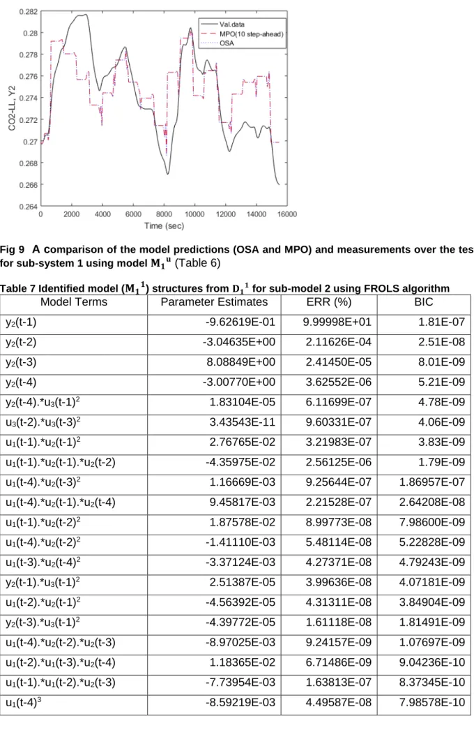
The details of the models for sub-system 2, obtained from each model term dictionary based on FROLS algorithm, are summarized in Tables 6-9. OSA predictions and the multi-step (10) prediction outputs (MPO) generated by these models, together with the true values (i.e. the system output measurements as test data), are shown in Figs. 9-12, respectively. Also, the prediction efficiency for each identified model is tabulated in Table 10.
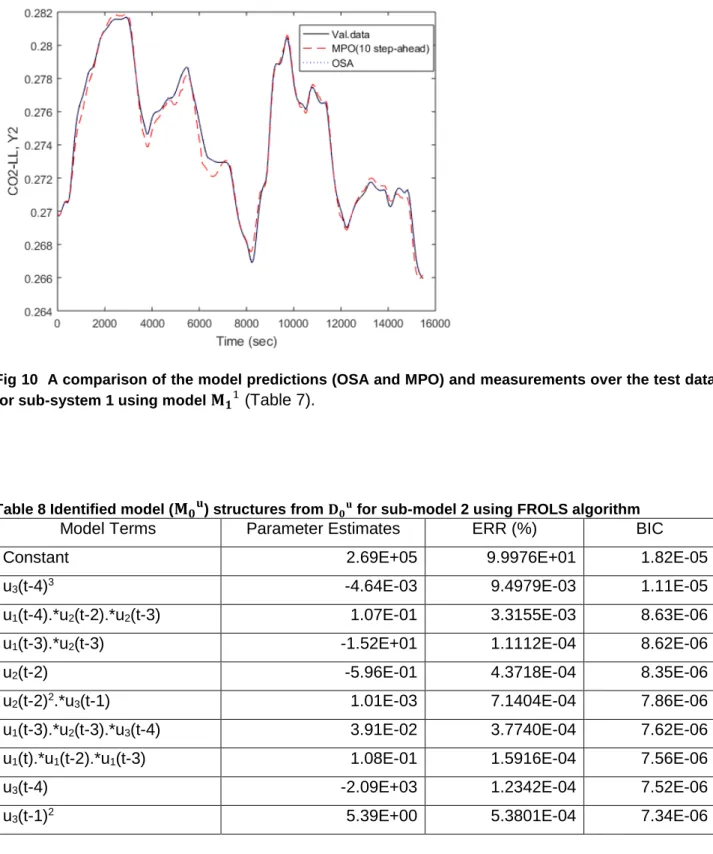
It was observed from Table 10 that M (obtained from D ) out-performed the other 3 models with a prediction efficiency of 99.996% and 99.295% based on OSA prediction and MPO (see Fig.10) and was selected as a suitable model to predict the CO2 loading at lean solvent stream to the
absorber. Thus, from Table 7, the model should be written as:
(14)
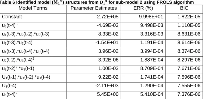
Table 6 Identified model ( ) structures from for sub-model 2 using FROLS algorithm
Model Terms Parameter Estimates ERR (%) BIC
Constant 2.72E+05 9.998E+01 1.822E-05
u3(t-4)3 -4.69E-03 9.498E-03 1.110E-05
u1(t-3).*u2(t-2).*u2(t-3) 8.33E-02 3.316E-03 8.631E-06
u1(t-3).*u2(t-4) -1.54E+01 1.191E-04 8.614E-06
u1(t-3).*u2(t-4).*u3(t-4) 3.96E-02 3.994E-04 8.374E-06
u2(t-2).*u3(t-4)2 -3.92E-06 1.887E-04 8.297E-06
u2(t-2)2.*u3(t-1) 1.00E-03 8.709E-04 7.671E-06
U1(t-1).*u1(t-2).*u1(t-4) 9.22E-02 1.741E-04 7.596E-06
U3(t-4) -2.11E+03 1.290E-04 7.555E-06
18
Fig 9 A comparison of the model predictions (OSA and MPO) and measurements over the test data for sub-system 1 using model (Table 6)
Table 7 Identified model ( ) structures from for sub-model 2 using FROLS algorithm
Model Terms Parameter Estimates ERR (%) BIC
y2(t-1) -9.62619E-01 9.99998E+01 1.81E-07
y2(t-2) -3.04635E+00 2.11626E-04 2.51E-08
y2(t-3) 8.08849E+00 2.41450E-05 8.01E-09
y2(t-4) -3.00770E+00 3.62552E-06 5.21E-09
y2(t-4).*u3(t-1)2 1.83104E-05 6.11699E-07 4.78E-09
u3(t-2).*u3(t-3)2 3.43543E-11 9.60331E-07 4.06E-09
u1(t-1).*u2(t-1)2 2.76765E-02 3.21983E-07 3.83E-09
u1(t-1).*u2(t-1).*u2(t-2) -4.35975E-02 2.56125E-06 1.79E-09
u1(t-4).*u2(t-3)2 1.16669E-03 9.25644E-07 1.86957E-07
u1(t-4).*u2(t-1).*u2(t-4) 9.45817E-03 2.21528E-07 2.64208E-08
u1(t-1).*u2(t-2)2 1.87578E-02 8.99773E-08 7.98600E-09
u1(t-4).*u2(t-2)2 -1.41110E-03 5.48114E-08 5.22828E-09
u1(t-3).*u2(t-4)2 -3.37124E-03 4.27371E-08 4.79243E-09
y2(t-1).*u3(t-1)2 2.51387E-05 3.99636E-08 4.07181E-09
u1(t-2).*u2(t-1)2 -4.56392E-05 4.31311E-08 3.84904E-09
y2(t-3).*u3(t-1)2 -4.39772E-05 1.61118E-08 1.81491E-09
u1(t-4).*u2(t-2).*u2(t-3) -8.97025E-03 9.24157E-09 1.07697E-09
u1(t-2).*u1(t-3).*u2(t-4) 1.18365E-02 6.71486E-09 9.04236E-10
u1(t-1).*u1(t-2).*u2(t-3) -7.73954E-03 1.63813E-07 8.37345E-10
19
Fig 10 A comparison of the model predictions (OSA and MPO) and measurements over the test data for sub-system 1 using model (Table 7).
Table 8 Identified model ( ) structures from for sub-model 2 using FROLS algorithm
Model Terms Parameter Estimates ERR (%) BIC
Constant 2.69E+05 9.9976E+01 1.82E-05
u3(t-4)3 -4.64E-03 9.4979E-03 1.11E-05
u1(t-4).*u2(t-2).*u2(t-3) 1.07E-01 3.3155E-03 8.63E-06
u1(t-3).*u2(t-3) -1.52E+01 1.1112E-04 8.62E-06
u2(t-2) -5.96E-01 4.3718E-04 8.35E-06
u2(t-2)2.*u3(t-1) 1.01E-03 7.1404E-04 7.86E-06
u1(t-3).*u2(t-3).*u3(t-4) 3.91E-02 3.7740E-04 7.62E-06
u1(t).*u1(t-2).*u1(t-3) 1.08E-01 1.5916E-04 7.56E-06
u3(t-4) -2.09E+03 1.2342E-04 7.52E-06
20
Fig 11 A comparison of the model predictions (OSA and MPO) and measurements over the test data for sub-system 1 using model (Table 8)
Table 9 Identified model ( ) structures from for sub-model 2 using FROLS algorithm
Model Terms Parameter Estimates ERR (%) BIC
y2(t-1) -2.16623E+00 9.99998E+01 1.86957E-07
y2(t-2) -3.02998E+00 2.11626E-04 2.64208E-08
y2(t-3) 1.12774E+01 2.41450E-05 7.98600E-09
y2(t-4) -5.00591E+00 3.62552E-06 5.22828E-09
y2(t-4).*u3(t-1)2 3.15751E-05 6.11699E-07 4.79243E-09
u3(t-2)2.*u3(t-3) 3.60624E-11 9.60331E-07 4.07181E-09
u1(t-1).*u2(t)2 3.31495E-03 3.39815E-07 3.83477E-09
u1(t-3).*u2(t-3)2 -9.38304E-03 1.19311E-06 2.90460E-09
u1(t-3).*u2(t-1)2 2.35993E-02 1.27838E-06 1.88882E-09
u1(t-3).*u2(t-1).*u2(t-2) -2.78876E-02 8.30813E-07 1.22289E-09
u1(t-3).*u2(t-2).*u2(t-3) 1.00523E-02 9.42003E-08 1.15517E-09
y2(t-1).*u3(t-1)2 3.30630E-05 4.65104E-08 1.12598E-09
u1(t-2).*u1(t-3).*u2(t-3) 4.74655E-02 4.29128E-08 1.09919E-09
u1(t-1).*u1(t-2).*u2(t) 1.67865E-02 1.21565E-07 1.00512E-09
u1(t-2).*u1(t-3).*u2(t) -3.82933E-02 8.89176E-08 9.37308E-10
u1(t-1).*u1(t-2).* u2(t-3) -2.29989E-02 4.80071E-08 9.03550E-10
u1(t-1)3 -4.88360E-03 2.64740E-08 8.87858E-10
21
Fig 12 . A comparison of the model predictions (OSA and MPO) and measurements over the test data for sub-system 1 using model (Table 9).
Table 10 VAF (and PE) for the Identified sub-model 2 (OSA and MPO)
Identified Models OSA (%VAF) MPO (%VAF)
M 42.2227 42.2227
M 99.9971 98.8362
M 42.2227 42.2227
M 99.9941 98.0601
5.3 Statistical Analysis
Statistical analysis was carryout on the suitable NARX models obtained using FROLS algorithm to represent the underlying dynamics between key variables in the solvent-based CO2 capture plant.
Table 11 shows the values of R, R2 and adjusted R2 of the identified models. R, which is the multiple
correlation coefficient, is a measure of how much the combination of model terms in each identified model correlates with the respective output variables. The R2 represents the portion of variance in
the response variable that is explained by the combination of model terms, while the adjusted R2 is
a measure of the accuracy of a model across different samples. R, R2 and adjusted R2 are calculated
as follows:
(15)
(16)
22
where is the measured output; is the multi-step ahead prediction; is the sum of squares error; is the total sum of squares; is the number of observations and is the number of terms. The R-value for sub-model1 (1.000) and sub-model 2 (1.000) indicates that the combination of model terms in each identified model are highly correlated with the response variables. The R2 value signifies that model 1 can explain 99.80% of the variation in the concentration
of CO2 in wt% at the absorber gas outlet and model 2 can explain 99.58% of the variation in CO2
lean loading at the lean solvent stream to the absorber. The values of adjusted R2 indicates that the
identified NARX models has high accuracy of prediction even across different samples. Table 11 Statistical performance of the identied Narx Model
Identified Model
Sub-model 1 1.0000 0.9980 0.9980
Sub-model 2 1.0000 0.9958 0.9957
6 Conclusion and Recommendations
In this study, a parsimonious polynomial NARX model was developed to predict the dynamic responses of an amine based PCC plant (3-inputs and 2-outputs) using the FROLS-ERR algorithm. The amine based PCC plant was represented as two MISO sub-systems (3-inputs and 2-outputs). The FROLS-ERR algorithm proved to be a powerful tool in selecting the most significant model terms for representing and predicting the response variables (CO2-MP and CO2–LL). These model terms
were ranked based on ERR. This gives a simple and transparent mathematical representation of the systems where we can clearly know how the system outputs depend on the variables and their interactions.
Identified models obtained from the different model term dictionaries were compared, in which the best model was selected based on the performance of multi-step ahead prediction output (MPO) and one-step ahead prediction (OSA). M and M gave the best performances based on the prediction efficiency of both OSA and MPO for both subsystem-1 and subsystem-2. Further statistical analysis indicated that the identified NARX models captures the underlying dynamics of the sub-systems. Multivariable control analysis of the capture process using the identified NARX models will be studied in the future.
Acknowledgment
The authors acknowledge financial support from EU FP7 Marie Curie International Research Staff Exchange Scheme (IRSES) (Ref: PIRSES-GA-2013-612230); The Engineering and Physical Sciences Research Council (EPSRC) under Grant EP/I011056/1; and Platform Grant EP/H00453X/1.
23 Reference
[1] Lawal A, Wang M, Stephenson P, Koumpouras G, Yeung H. Dynamic modelling and analysis of post-combustion CO2 chemical absorption process for coal-fired power plants. Fuel
2010;89:2791–801.
[2] Huaman RNE, Jun TX. Energy related CO2 emissions and the progress on CCS projects: a
review. Renew Sustain Energy Rev 2014;31:368–85.
[3] Wang M, Lawal A, Stephenson P, Sidders J, Ramshaw C. Post-combustion CO2 capture with
chemical absorption: a state-of-the-art review. Chem Eng Res Des 2011;89:1609–24.
[4] Mumford KA, Wu Y, Smith KH, Stevens GW. Review of solvent based carbon-dioxide capture technologies. Front Chem Sci Eng 2015;9:125–41.
[5] Mac Dowell N, Staffell I. The role of flexible CCS in the UK’s future energy system. Int J Greenh Gas Control 2015.
[6] Bui M, Gunawan I, Verheyen V, Feron P, Meuleman E, Adeloju S. Dynamic modelling and optimisation of flexible operation in post-combustion CO2 capture plants—A review. Comput
Chem Eng 2014;61:245–65.
[7] Lawal A, Wang M, Stephenson P, Yeung H. Dynamic modelling of CO2 absorption for post
combustion capture in coal-fired power plants. Fuel 2009;88:2455–62.
[8] Lawal A, Wang M, Stephenson P, Obi O. Demonstrating full-scale post-combustion CO2
capture for coal-fired power plants through dynamic modelling and simulation. Fuel 2012;101:115–28.
[9] Biliyok C, Lawal A, Wang M, Seibert F. Dynamic Validation of Model for Post-Combustion Chemical Absorption CO2 Capture Plant. Comput Aided Chem Eng 2012;30:807–11.
[10] Biliyok C, Lawal A, Wang M, Seibert F. Dynamic modelling, validation and analysis of post-combustion chemical absorption CO2 capture plant. Int J Greenh Gas Control 2012;9:428–
45.
[11] Mac Dowell N, Samsatli NJ, Shah N. Dynamic modelling and analysis of an amine-based post-combustion CO2 capture absorption column. Int J Greenh Gas Control 2013;12:247–58.
[12] Mac Dowell N, Shah N. Dynamic modelling and analysis of a coal-fired power plant integrated with a novel split-flow configuration post-combustion CO2 capture process. Int J Greenh Gas
Control 2014;27:103–19.
[13] Oko E, Wang M, Olaleye AK. Simplification of detailed rate-based model of post-combustion CO2 capture for full chain CCS integration studies. Fuel 2015;142:87–93.
[14] Peng J, Edgar TF, Eldridge RB. Dynamic rate-based and equilibrium models for a packed reactive distillation column. Chem Eng Sci 2003;58:2671–80.
[15] Dunia R, Rochelle GT, Qin SJ. Subspace system identification for CO2 recovery processes.
Proc. IEEE Int. Symp. Comput. Control Syst. Des., Department of Chemical Engineering, University of Texas, Austin, TX 78712, United States Department of Chemical Engineering and Material Sciences, University of Southern California, CA 90089, United States: 2011, p. 846–51.
[16] Nittaya T, Douglas PL, Croiset E, Ricardez-Sandoval LA. Dynamic Modelling and Controllability Studies of a Commercial-scale MEA Absorption Processes for CO2 Capture
from Coal-fired Power Plants. 12th Int Conf Greenh Gas Control Technol GHGT-12 2014;63:1595–600.
[17] He Z, Sahraei MH, Ricardez-Sandoval LA. Flexible operation and simultaneous scheduling and control of a CO2 capture plant using model predictive control. Int J Greenh Gas Control
2016;48:300–11.
24
operation of amine-based post-combustion CO2 capture systems. Int J Greenh Gas Control
2015;39:377–89.
[19] Hossein Sahraei M, Ricardez-Sandoval LA. Controllability and optimal scheduling of a CO2
capture plant using model predictive control. Int J Greenh Gas Control 2014;30:58–71. [20] Mehleria ED, Mac Dowella N, Thornhillb NF. Model Predictive Control of Post-Combustion
CO2 Capture Process integrated with a gas-fired power plant. PSE2015 ESCAPE25 n.d.:27.
[21] Abdul Manaf N, Cousins A, Feron P, Abbas A. Dynamic modelling, identification and preliminary control analysis of an amine-based post-combustion CO2 capture pilot plant. J
Clean Prod 2016;113:635–53.
[22] Sipöcz N, Tobiesen FA, Assadi M. The use of Artificial Neural Network models for CO2 capture
plants. Appl Energy 2011;88:2368–76.
[23] Li F, Zhang J, Oko E, Wang M. Modelling of a post-combustion CO2 capture process using
neural networks. Fuel 2015;151:156–63.
[24] Li F, Zhang J, Oko E, Wang M. Modelling of a post-combustion CO2 capture process using
extreme learning machine. Int J Coal Sci Technol 2017;4:33–40.
[25] Ayala Solares JR, Wei HL, Boynton RJ, Walker SN, Billings SA. Modeling and prediction of global magnetic disturbance in near-Earth space: A case study for Kp index using NARX models. Sp Weather 2016;14:899–916.
[26] Roy RJ, Sherman J. A Learning Technique for Volterra Series Representation. IEEE Trans Automat Contr 1967;AC-12:761–4.
[27] Fu FC, Farison JB. On the Volterra-series functional identification of non-linear discrete-time systems. Int J Control 1973;18:1281–9.
[28] Bard Y, Lapidus L. Nonlinear System Identification. Ind Eng Chem Fundam 1970;9:628–33. [29] Schetzen M. Nonlinear System Modeling Based on the Wiener Theory. Proc IEEE
1981;69:1557–73. doi:10.1109/PROC.1981.12201.
[30] Billings SA. Nonlinear system identification: NARMAX methods in the time, frequency, and spatio-temporal domains. 2013.
[31] Leontaritis IJ, Billings SA. Input-output parametric models for non-linear systems Part I: Deterministic non-linear systems. Int J Control 1985;41:303–28.
[32] Chen S, Billings SA. Extended model set, global data and threshold model identification of severely non-linear systems. Int J Control 1989;50:1897–923.
[33] Wei HL, Billings SA, Liu J. Term and variable selection for non-linear system identification. Int J Control 2004;77:86–110. doi:10.1080/00207170310001639640.
[34] Wei HL, Billings SA. Model structure selection using an integrated forward orthogonal search algorithm assisted by squared correlation and mutual information. Int J Model Identif Control 2008;3:341–56.
[35] Dantas TSS, Franco IC, Fileti AMF, Da Silva F V. Nonlinear system identification of a refrigeration system. Int J Air-Conditioning Refrig 2016;24.
[36] Gu Y, Wei H-L. Significant Indicators and Determinants of Happiness: Evidence from a UK Survey and Revealed by a Data-Driven Systems Modelling Approach. Soc Sci 2018;7:53. [37] Johansen TA, Brustad AF, Andersen TS, Kristiansen R. Nonlinear system identification of
fixed wing UAV aerodynamics. Proc. IASTED Int. Conf. Model. Identif. Control, vol. 830, 2016, p. 44–51. doi:10.2316/P.2016.830-026.
[38] Macedo MMG, Takimura CK, Lemos PA, Gutierrez MA. An automatic labeling bifurcation method for intracoronary optical coherence tomography images. Prog. Biomed. Opt. Imaging - Proc. SPIE, vol. 9417, 2015.
25
[39] Billings SA, Korenberg MJ, Chen S. Identification of non-linear output-affine systems using an orthogonal least-squares algorithm. Int J Syst Sci 1988;19:1559–68.
[40] Billings SA, Chen S, Korenbergs MJ. Identification of mimo non-linear systems using a forward-regression orthogonal estimator. Int J Control 1989;49:2157–89.
[41] Zhu Y. Multivariable system identification for process control. Elsevier; 2001.
[42] Wei HL, Billings SA. Improved model identification for non-linear systems using a random subsampling and multifold modelling (RSMM) approach. Int J Control 2009;82:27–42.