Generative pairwise models for speaker recognition

(1)

Politecnico di Torino

Porto Institutional Repository

[Proceeding] Generative pairwise models for speaker recognition

Original Citation:

Cumani S., Laface P. (2014).

Generative pairwise models for speaker recognition.

In: Odyssey

2014: The Speaker and Language Recognition Workshop, Joensuu, Finland, 16-19 June 2014. pp.

273-279

Availability:

This version is available at :

http://porto.polito.it/2551354/

since: June 2014

Publisher:

International Speech Communication Association

Terms of use:

This article is made available under terms and conditions applicable to Open Access Policy Article

("Public - All rights reserved") , as described at

http://porto.polito.it/terms_and_conditions.

html

Porto, the institutional repository of the Politecnico di Torino, is provided by the University Library

and the IT-Services. The aim is to enable open access to all the world. Please

share with us

how

this access benefits you. Your story matters.

(2)

Generative pairwise models for speaker recognition

Sandro Cumani, and Pietro Laface

{Sandro.Cumani, Pietro.Laface}@polito.it

Abstract

This paper proposes a simple model for speaker recognition based on i–vector pairs, and analyzes its similarity and dif-ferences with respect to the state–of–the–art Probabilistic Lin-ear Discriminant Analysis (PLDA) and Pairwise Support Vector Machine (PSVM) models. Similar to the discriminative PSVM approach, we propose a generative model of i–vector pairs, rather than an usual i–vector based model. The model is based on two Gaussian distributions, one for the “same speakers” and the other for the “different speakers” i–vector pairs, and on the assumption that the i–vector pairs are independent. This inde-pendence assumption allows the distributions of the two classes to be independently estimated. The “Two–Gaussian” approach can be extended to the Heavy–Tailed distributions, still allow-ing a fast closed form solution to be obtained for testallow-ing i–vector pairs. We show that this model is closely related to PLDA and to PSVM models, and that tested on the female part of the tel– tel NIST SRE 2010 extended evaluation set, it is able to achieve comparable accuracy with respect to the other models, trained with different objective functions and training procedures.

1. Introduction

The current state–of–the–art in speaker recognition is based on a low–dimensional representation of a speech segment, the so– called i–vector [1, 2], in combination with Probabilistic Linear Discriminant Analysis (PLDA) generative models [3, 4, 5]. An i–vector is a compact representation of a speech segment, ob-tained from the statistics of a Gaussian Mixture Model (GMM) supervector [6] by a Maximum a Posteriori point estimate of a posterior distribution [2]. A PLDA classifier models the un-derlying distribution of the speaker and channel components of the i–vectors in a probabilistic framework. From these distri-butions it is possible to evaluate the likelihood ratio between the “same speaker” hypothesis and “different speaker” hypoth-esis for a pair of i–vectors. The same paradigm can be used to train discriminative systems where the observation patterns are pairs of i–vectors. In particular discriminative linear classi-fiers, based on Pairwise Support Vector Machine (PSVM) [7, 8] and on logistic regression [9] have been proposed, which have been shown to achieve state–of–the–art results on recent NIST evaluations [10, 11].

In this paper we propose a simple generative model for speaker recognition based on i–vector pairs. The model is based on two Gaussian distributions, one for the “same speaker” i– vector pairs and the other for the “different speaker” pairs, and on the assumption that the i–vector pairs are independent. We illustrate the structure of the precision matrices of the two distri-butions, and we detail how their parameters can be effectively estimated. Moreover, since the independence assumption al-lows the distributions of the two classes to be independently Computational resources for this work were provided by HPC@POLITO (http://www.hpc.polito.it) Politecnico di Torino, Italy

estimated, our “Two–Gaussian” model, referred to in the fol-lowing as 2–GAU, can be easily extended to Heavy–Tailed dis-tributions leading to the “Two–Heavy–Tailed” (2–HT) model.

We also show that the proposed model is closely related to PLDA and to PSVM models, and that tested on the female part of the tel–tel NIST SRE 2010 extended evaluation set, it is able to achieve comparable accuracy with respect to the other models, trained with different objective functions and training procedures. Although we do not claim that this simple model is more accurate than its state–of–the–art competitors, it has the merit of shedding some light on the pairwise classifiers, reveal-ing a possible unifyreveal-ing framework, despite relevant variations about the model assumptions, the estimation procedures, and the objective functions that each model optimizes.

The paper is organized as follows: Section 2 and 3 briefly recall the PLDA and PSVM models, their parameters, and their objective functions. Section 4 presents the 2–GAU model and illustrates a very fast training procedure for estimating its pa-rameters. Section 5 shows the similarity of the Gaussian PLDA and PSVM models with the 2–GAU model. Section 6 extends the 2–GAU model leading to the 2–HT model, and presents an effective approach for training this more complex model, to-gether with considerations about its training and testing com-plexity. In Section 7 the similarities and differences of the clas-sifiers are illustrated by using artificial uni–dimensional data. Section 8 is devoted to the illustration of the experimental re-sults, and conclusions are drawn in Section 9.

2. Gaussian PLDA

The generative Gaussian PLDA models [12, 3] are among the best models for comparison of i–vectors. In this section we briefly recall the Gaussian PLDA framework, and also the “Two–covariance model” [4, 5], which provides a useful inter-pretation of the PSVM approach described in Section 3.

2.1. PLDA

The i–vector generation process is described in the PLDA ap-proach by means of a latent variable probabilistic model where an i–vectorφiis represented as the sum of three factors, namely a speaker factory, an inter–session (channel) factorxiand a residual noiseias:

φi=m+Uy+Vxi+i. (1) MatricesUand Vtypically constrain the speaker and inter– session factors to be of lower dimension than the i–vectors space. PLDA estimates the distribution of the latent variables that maximize the likelihood of the observed i–vectors, assum-ing that i–vectors from the same speaker share the same speaker factor, i.e., the same value for latent variabley[3]. The simplest PLDA model assumes that all the hidden variables are Gaussian distributed, and that the noise termihas a full covariance ma-trix, so that the termsVxiandiin (1) can be merged. Thus,

(3)

an i–vectorφiis re–defined as:

φi=m+Uy+i, (2) where the speaker factoryand the residual noise are distributed as:

y∼ N(0,I) i∼ N(0,Λ

−1

), (3)

andΛis the precision matrix of noisei.

2.2. Two–covariance model

Further simplification of the PLDA model (2) is obtained as-suming that the speaker and inter–session subspaces span the entire i–vector space. This simplified model, referred to as the Two–covariance model [4, 5], or 2–COV for short, accounts for two Gaussian–distributed components: the speaker component

y, and the inter–session variability componenti, which are combined to produce an i–vector as:

φi=m+y+i, (4) where

y∼ N(0,B−1) i∼ N(0,W−1), (5) and B−1

and W−1

are the between–speaker and within– speaker covariance matrix, respectively.

It has been shown in [7] that the 2–COV model log– likelihood ratio for an i–vector pair is a quadratic function, in-variant to i–vector swapping, which can be formulated as:

s(φ1,φ2) = φT1Λφ2+φT2Λφ1+φT1Γφ1+φT2Γφ2

+(φ1+φ2)Tc+k , (6)

where the within-speaker and between–speaker covariances are related toΛ,Γ,candkaccording to:

Λ= 1 2W T_˜ ΛW Γ=1 2W T ( ˜Λ−_Γ˜₎_W c=WT( ˜Λ−Γ˜)Bµ k= ˜k+1 2 h (Bµ)T( ˜Λ−2 ˜Γ)Bµi, (7) with ˜ Λ= (B+ 2W)−1 Γ˜= (B+W)−1 ˜

k= 2 log|Γ˜| −log|B| −log|Λ˜|+µT_Bµ_.

3. PSVM

A successful alternative to generative PLDA models has been presented in [7, 8], where a pairwise SVM model has been pro-posed, which is trained to discriminate between “same speaker” and “different speaker” pairs. This is in contrast with the usual “one-versus-all” framework, where an SVM model is created for each enrolled speaker, using as samples of the impostor class the utterances of a background cohort of speakers. This approach avoids the major weakness of “one-versus-all” SVM training, namely the scarcity of available samples for the target speakers.

In [7] it has been shown that the score of a second order Taylor expansion of an i–vector pairΦ= (φ1,φ2)can be

for-mulated as a functions(Φ), invariant to i–vector swapping, and that it leads to the same formulation of the 2–COV score (6). In particular, the second order Taylor expansion fors(Φ)around pointΦˆ =0is:

s(Φ) =s( ˆΦ) + (Φ·∇s|Φˆ) +Φ

T

(H(s)|Φˆ)Φ, (8)

where∇is the vector of differential operators

∇= ∂ ∂Φ1 , . . . , ∂ ∂Φd ,

dis the dimension of the i–vector pair, andH(s)is the Hessian of functions(Φ). Defining: s( ˆΦ) =k , ∇s|Φˆ = [c c], H(s)|Φˆ = Γ Λ Λ Γ , (9)

with a symmetricΛ, we obtain the quadratic function of the i–vector pair: s(φ1,φ2) = φ T 1Λφ2+φ T 2Λφ1+φ T 1Γφ1+φ T 2Γφ2 +(φ1+φ2) T c+k , (10) which is identical to (6), but with matricesΛandΓ, and vec-torc, estimated by means of a different objective function and training procedure. It is worth noting that the structure of (9) naturally arises from the symmetries of the problem (see Sec-tion III-E in [7]).

4. Generative Two–Gaussian model

The goal of PLDA, and of the other classifiers of the same fam-ily, is to model the distribution of the speaker and channel com-ponents of the ivectors. We propose, instead, to directly charac-terize the ivectors pairsΦij=

φi φj by a simple generative Gaussian model.

Our main assumption is that the i–vector pairs, given their labels, are independently generated from the two Gaussian dis-tributions: ΦSij∼ N(µS,Λ −1 S ) Φ D ij∼ N(µD,Λ −1 D ), (11) whereS andDrefer to “same speaker” and “different speak-ers”, respectively. This assumption is not accurate, because the complete set of i–vector pairs of a training dataset are, by def-inition, correlated. However, this working hypothesis allows obtaining a relevant simplification of the models.

The speaker verification log–likelihood ratio is simply com-puted as:

logR= logN(Φij|µS,Λ

−1

S )−logN(Φij|µD,Λ

−1

D ). (12) A second assumption is that the two distributions have the same mean, i.e.,µ_S=µ_D.

Recalling that the i–vector pair likelihoods must be invariant to i–vector swapping, the covariance matricesΛ−_S1andΛ−_D1must obey the following symmetry constraints:

Λ−S1= AS BS BS AS Λ−D1= AD BD BD AD (13) where,A∗andB∗are symmetric, and the mean of the

distri-butionsµ=µS =µDare defined asµ=

m m

,mbeing a vector of the same dimensions of an i–vector. Although we expect thatBD ≈0, because the i–vectors should be uncorre-lated, we do estimate this matrix from the data.

The equations for trainingADandBDare illustrated in the next subsection, devoted to their estimation.

(4)

4.1. 2–GAU model training

The 2–GAU models are trained by maximizing the likelihood of the training pairs, under the i–vector pair independence assump-tion. Although the number of training pairs is huge, because it grows quadratically with the number of i–vectors, we here pro-vide a fast solution that allows estimating the parameters of the 2–GAU model even with very large set of data. For the sake of clarity we assume that i–vectors have been centered, so that the mean of the two distributions isµ=0, butµcan be easily re–estimated extending the techniques detailed in the following.

LetδijSandδ D

ijdenote the indicator functions for the “same speaker” and “different speaker” pair classes, respectively:

δijS =

1 ifφi,φjbelong to “same speaker” class

0 otherwise

δDij= 1−δ S

ij. (14)

Maximum Likelihood estimate of the 2-GAU distribution pa-rameters can be obtained in closed form [13] as:

Λ−S1= 1 NS X i,j δSijΦijΦTij Λ−D1= 1 ND X i,j δDijΦijΦTij (15)

whereNSandNDdenote the number of “same–speaker” and “different speaker” pairs, respectively.

The “different speaker” covariance,Λ−_D1, can be alternatively computed as: Λ−D1= 1 ND NTΛ−T1−NSΛ−S1 , (16) where Λ−T1= 1 NT X i,j ΦijΦTij. (17)

is the total covariance matrix of the pairs, andNTis the number of pairs.

Direct computation ofΛ−_S1andΛ−_D1by means of (15) en-tails a summation over all training pairs, which would have an overwhelming complexity ofO(N2_d2₎

, whereNanddare the number and the dimension of the i–vectors, respectively. How-ever, by exploiting the block structure of (13), these covariances can be efficiently obtained. The “same–speaker” covariance,

Λ−_S1, is compose of the blocks matricesASandBScomputed as: AS= 1 NS X i,j δSijφiφ T i BS= 1 NS X i,j δSijφiφ T j . (18)

Sinceδij = 1for all pairs belonging to speakers, (18) can be rewritten, by substituting summations over the pairs with sum-mations over the speakers, as:

wheresdenotes the set of i–vectors belonging to a speaker, and |s|is its cardinality.

The total covariance matrixΛ−T1can be obtained from block matricesATandBT. By analogy with (19), we get:

AT = 1 NT X i Nφ_iφT_i BT = 1 NT X i φ_i ! X j φ_j !T , (20)

andΛ−D1is obtained from (16).

Computing these statistics by using (19) and (20) has complex-ityO(N d2), i.e., is linear with the number of i–vectors, thus very fast even for large datasets.

It is worth noting that these estimates are closely related to the i–vector within class and total covariances. However, since we maximize the likelihood of i–vector pairs, speakers providing more utterances have larger impact on the estimation of the co-variances, as can be observed looking at matricesATandBT.

5. Relation to the PLDA and PSVM models

In the following we show that the 2–GAU model is closely re-lated to the 2–COV and PSVM models.

5.1. Relation to PLDA

Let’s recall that, if the noise termihas full covariance matrix, an i–vector is generated in the PLDA model according to (2), where i–vectors from the same speaker share the same value for the hidden variabley. Thus, a pair of “same speaker” i–vectors, i.e., a pair sharing a singley, is modeled as:

ΦSij= φi φ_j = m m + U U y+ i j , (21)

whereas, a “different speaker” i–vector pair is modeled as:

ΦDij= φi φ_j = m m + U 0 0 U yi yj + i j . (22) Since each model is a linear combination of Gaussian– distributed variables, closed–form integration over the speaker variables is possible, which gives:

ΦS∼ N(µ,Λ −1 S ) ,ΦD∼ N(µ,Λ −1 D ), (23) where Λ−S1 = UUT+Λ−1 UUT UUT _UUT₊_Λ−1 Λ−D1 = UUT+Λ−1 0 0 UUT₊_Λ−1 , (24)

andΛis the noise precision matrix. Comparing (23) and (24) with (11) and (13), respectively, it can be observed that the PLDA model estimates a constrained solution for the covari-ance matrices of the 2–GAU model. However, the parameters of the PLDA model are estimated by maximizing the likelihood of the training i–vectors, whereas the parameters of the 2–GAU model are estimated by maximizing the likelihood of the train-ing i–vector pairs. Although our original assumption - that the i–vector pairs, given their labels, are independent and identi-cally distributed random variables - is not accurate, it will be shown in Section 8, devoted to the experiments, that it is does not affect the model accuracy.

(5)

5.2. Relation to PSVM

The PSVM approach was introduced as a discriminatively trained model derived from the 2–COV in [7], where it was shown that the scoring functions of the PSVM and of the 2– COV models are formally equivalent. This equivalence has also been stated without reference to the 2–COV model, as it has been recalled in Section 3. The 2–GAU model allows providing a novel interpretation of the PSVM scoring function. Devel-oping the log–likelihood ratio of the 2–GAU model (12), and recalling thatµ=µS=µD, from (12) one gets:

logR=k−1 2(Φij−µ) T ΛS(Φij−µ) +1 2(Φij−µ) T ΛD(Φij−µ) =k+1 2(Φij−µ) T (ΛD−ΛS) (Φij−µ) = ˜k+ΦTijc+ 1 2Φ T ijHΦij, (25) where H = ΛD −ΛS, c = −Hµ, and˜k collects all the terms that do not depend on the i–vector pairΦij. Comparing (25) with (8) we can observe that the two expression are for-mally equivalent. We can thus interpret the PSVM framework as a discriminative approach for estimating the difference of the precision matricesΛD−ΛS, and the (shared) mean of the dis-tributions of our 2–GAU model.

6. Two–Heavy–Tailed Model

The simplest PLDA model assumes a Gaussian distribution for the prior parameters. However, in [3] it has been shown that ML estimation of the PLDA parameters under a Gaussian assump-tion fails to produce accurate models for i-vectors that are not length–normalized. Thus, Heavy–Tailed distributions for the model priors have been proposed leading to the Heavy-Tailed PLDA model (HT–PLDA). A similar assumption for the prior distribution can be used to model i–vector pairs leading to the Two–Heavy–Tailed distribution model. In particular, for each i–vector pair, we define a hidden variableνijthat is assumed to be an i.i.d. random variable generated from a Gamma distribu-tion depending on the pair label as:

νij,S∼Γ a_S 2 , aS 2 νij,D∼Γ a_D 2 , aD 2 , (26) whereS,Ddenote the “same speaker” and “different speaker” hypothesis, andaS,aD are the parameters of the two Gamma distributions, respectively. We also assume that the pairs are i.i.d. distributed, given the pair label and the hidden variables, according to the Gaussian distributions:

ΦSij∼ T(µS,ΛS, aS) ΦDij∼ T(µD,Λ

−1

D , aD), (28) withaS andaDdegrees of freedom, respectively. The likeli-hood ratio of an i–vector pair can then be computed as the ratio between two t–distributions. It is worth noting that, in contrast with the other models, the separation surfaces produced by the 2–HT model are not constrained to be quadratic, but can have more general shapes.

6.1. Relation with the HT–PLDA model

The 2–HT model has many similarities with the HT–PLDA model. In particular, we can show that the HT–PLDA model, with some additional constraints, formally corresponds to a slight simplification of the 2-HT model in (27). The HT–PLDA model assumes, as in (1), that an i–vector is generated according to:

φ_i=m+Uy+Vxi+ ¯i, (29) but with these distributions:

y|u1∼ N(0,Iu−11), u1∼Γ( a1 2, a1 2) xi|u2i∼ N(0,Iu −1 2i ), u2∼Γ( a2 2, a2 2) ¯ i|νi∼ N(0,Λ¯ −1 νi−1), νi∼Γ( b 2, b 2), (30)

whereu1,u2iandνiare independently distributed hidden vari-ables, anda1,a2andbare the parameters of the prior distribu-tions foru1,u2iandνi, respectively.

We can simplify the HT–PLDA model assuming that, for every speaker,νi = u1andu2i =u1 regardless of the utter-ance, withu∼Γ(a

2,

a

2). This simplification violates the

inde-pendence assumptions of PLDA because it makes the priors for the speaker and channel factors dependent. However, it allows us to integrate over the hidden variables and, since the termsVx

andΛ¯−1have the same precision matrix scaling factor, they can be merged into a single termi withΛ−1 = ¯Λ

−1 +VVT , leading to: φi=m+Uy+i, (31) where y∼ T(0,I, a) i∼ T(0,Λ −1 , a) (32)

In analogy with (11), the distributions for “same speaker” and “different speaker” i–vector pairs can be written as:

ΦSij∼ T(µS,Λ −1 S , a) Φ D ij∼ T(µD,Λ −1 D , a), (33) whereΛSandΛDare given by (24).

Comparing (33) with (27) it easy verifying that the HT–PLDA model is formally equivalent to the proposed approach if we assume thatνij,S=νij,D=νij∼Γ(a₂,a₂)in (27).

Without the proposed simplification, the HT–PLDA model cannot be transformed in the 2–HT model (28), and the speaker verification log–likelihood ratio cannot be computed in closed form, thus making the HT–PLDA model much more expensive in testing than our proposed 2–HT model.

6.2. 2–HT model training

In contrast with the 2–GAU approach, the estimation of the 2– HT parameters does not have a closed form solution, thus we resort to Expectation-Maximization estimation.

We will illustrate only the estimation of the model parame-ters for the “same speaker” distribution because the same ap-proach can be used for estimating the parameters of the “differ-ent speaker” class.

6.2.1. Expectation step

The expectation step requires computing the posterior distribu-tion for theνij,Shidden variables, given the observations. Since

(6)

the Gamma distribution is a conjugate prior for the scaling fac-tor of the precision matrix of the i–vecfac-tor conditional distribu-tion, the posterior forνij,Sis again a Gamma distribution with parameters: νij,S,Φij ∼Γ aS+ 2d 2 , aS+ΦTijΛSΦij 2 ! , (34)

wheredis the i–vector dimension (2dis, thus, the i–vector pair dimension). The expectations necessary for the M–step are:

E[νij,S] = aS+ 2d aS+ΦTijΛSΦij E[logνij,S] =ψ( aS+ 2d 2 )−log aS+ΦTijΛSΦij 2 (35)

whereψ(·)denotes the digamma function.

6.2.2. Maximization step The objective to be maximized is:

X i,j

δSijE[logP(Φij, νij,S)] , (36)

which corresponds to solving the problem:

argmax ΛS,aS X i,j δSij 1 2log|ΛS| − 1 2E[νij,S]Φ T ijΛSΦij −log ΓaS 2 +aS 2 log aS 2 + _a_S 2 −1 E[logνij,S]− aS 2 E[νij,S] i . (37) The solution forΛSis given by:

Λ−S1 = 1 NS X i,j δijSE[νij,S]ΦijΦTij, (38)

The parameteraSis obtained as the solution of the equation:

logaS 2−ψ _a_S 2 = 1 NS X ij

δijS(E[νij,S]−E[logνij,S]−1) (39) which has no closed–form solution, thus it is solved numerically by using a line search algorithm.

ComputingΛ−_S1 by means of (38) is very expensive be-cause a single EM iteration hasO(N2_d2₎

computational com-plexity. However, (38) can be rewritten, in matrix form, as:

Λ−_S1= 1

NS

Θ(∆S◦N)ΘT, (40)

whereΘis the matrix of all i–vectorsΘ= [φ₁, . . . ,φ_N],∆S is the matrix defined as∆S i,j = δSij, N is matrix with ele-mentsNij = E[νij,S]and◦denotes the Hadamard product, so that the complexity of an EM iteration reduces toO(N2d). Although the training time for the 2–HT model remains much higher compared to the 2–GAU training time, the scoring com-plexity of the 2–HT model is comparable to the one the Gaus-sian models (and PSVM), because given the parameters, the dis-tributions in (28), and the corresponding likelihood ratios can be easily computed.

Directly modeling the distributions of the “same speaker” and “different speaker” i–vector pairs allows, thus, an easier

extension of the model to more complex distributions without incurring in expensive or even intractable formulations. Dif-ferent models can be devised to better capture the underlying distribution of the i–vector pairs, such as Mixture Models in-stead of single Gaussian or t–distributions. The effectiveness of these approaches, however, has not yet been experimentally validated.

7. Model comparison

An illustration of the similarities and differences of the models considered in this paper is summarized in Figures 1 ((a)–(i)). The figures show the contour levels1 of the scoring functions of the 2–COV, 2–GAU, PSVM, and 2–HT models, respectively. Darker areas correspond to higher scores for the “same class” hypothesis. The dots represent training pairs of a set of data randomly generated from Heavy–Tailed distributions. The fig-ures do not show the data, but pairs of data, identified by their associated label: white for “same class” and black for “differ-ent class”. The PLDA model is equival“differ-ent to the 2–COV model because no subspace dimension reduction is possible for uni– dimensional data, thus it is not represented in these figures.

The contour plots clearly show that different separation re-gions are used by the classifiers. In particular, the 2–COV, 2– GAU, and PSVM classifiers have all quadratic shape separation regions, but they differ due to the different objective function that is optimized for each model. The shape of the separation regions for 2-HT model is not quadratic, and has, for this ex-ample, a sharper distribution of its log–likelihood ratio scores.

8. Experiments

The models have been tested on the female part of the tel-tel ex-tended NIST 2010 evaluation trials [10] using a front–end based on 60-dimensional cepstral features. In particular, the i-vector extractor is based on a 2048-component full covariance gender-independent UBM, and on a gender-dependentTmatrix. The UBM was trained on NIST SRE 2004, 2005 and 2006 data. The i–vector extractor has been trained from the same data, and in addition with Switchboard II Phases 2 and 3, Switchboard Cel-lular Parts 1 and 2, and Fisher datasets. For these experiments the dimension of the i-vectors was set tod= 400. All classifiers were trained with the complete set of data, excluding the Fisher dataset. The Gaussian PLDA system was implemented accord-ing to the framework illustrated in [3]. Since the 2–GAU and 2–HT models do not explicitly allow constraining the speaker space, Linear Discriminant Analysis (LDA) was used as an al-ternative approach for reducing the i–vector dimensions. The PLDA, 2–COV, and 2–GAU systems were trained with length– normalized i–vectors. Length–normalization was applied after mean removal and whitening of the i–vector covariance matrix. For the PLDA with low dimensional speaker subspace, covari-ance whitening was replaced by Within Class Covaricovari-ance Nor-malization (WCCN)2_{. For the PSVM system, the i–vector were}

whitened by WCCN, but no length–normalization was applied, as we did in the experiments illustrated in[7]. Finally, no nor-malization was applied for the 2–HT system.

1_{A strictly monotone non–linear transformation of the scores has}

been performed to enhance the image quality

2_{The discussion of the appropriateness of the use of WCCN, rather}

2 (h) 2–GAU 1.0 0.5 0.0 0.5 1.0

φ

1 1.0 0.5 0.0 0.5 1.0

φ

2 (i) PSVM

Figure 1: Contour plots of the scoring functions of different classifiers for a set of pairs of uni–dimensional data. Data were randomly generated from Heavy–Tailed distributions. The first set of images refers to easily separable classes, whereas the second set refers to more noisy data. The “same class” and “different class” pairs are represented by white and black dots, respectively. Darker areas correspond to higher scores for the “same class” hypothesis.

(8)

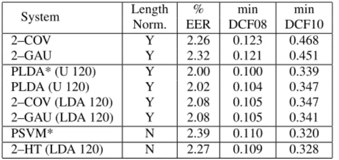
Table 1: Comparison of the performance of PLDA, PSVM, 2– COV, 2–GAU, and 2–HT models on the female part of the tel-tel extended NIST 2010 evaluation trials. Systems marked by “*” pre–process i–vectors by using WCCN rather than covariance whitening. If relevant, the dimension of speaker or LDA sub-space is given in parentheses.

System Length % min min

Norm. EER DCF08 DCF10 2–COV Y 2.26 0.123 0.468 2–GAU Y 2.32 0.121 0.451 PLDA* (U 120) Y 2.00 0.100 0.339 PLDA (U 120) Y 2.02 0.104 0.347 2–COV (LDA 120) Y 2.08 0.105 0.347 2–GAU (LDA 120) Y 2.08 0.105 0.341 PSVM* N 2.39 0.110 0.320 2–HT (LDA 120) N 2.27 0.109 0.328

Table 1 summarizes the performance of the evaluated mod-els on the female part of the extended telephone condition in the NIST 2010 evaluation. The recognition accuracy is given in terms of Equal Error Rate (EER) and Minimum Detection Cost Functions defined by NIST for the 2008 (minDCF08) and 2010 (minDCF10) evaluations [10]. The scores were not normal-ized. The first two lines compare the performance of the 2–GAU model with the 2–COV model, corresponding to a PLDA model without speaker subspace dimensionality reduction. The two models give similar results, thus the 2–GAU model assumption about i–vector pair independence does not have significant im-pact on the performance. Constraining the speaker subspace by using a low–rankUor LDA shows significant improvement of the performance for both systems. Again, the 2–GAU classifier performs as well as the PLDA or 2–COV systems. Although not shown in the Table, these systems perform much worse without i–vector length–normalization. On the contrary, as shown in the last two rows, the PSVM and the 2–HT classifiers are able to achieve similar results without length–normalization.

9. Conclusions

A simple generative Gaussian model has been proposed using as its observations ivectors pairs rather than the i-vectors. We have highlighted the relations of this classifier with other pairwise classifiers, and we have shown that this simple model is able to achieve results that are comparable to the others approaches. The extension of this approach to the Two–Heavy–Tailed model has not given so far appreciable advantages, although it does not require i–vector pre–processing except LDA. Further develop-ments are possible for the proposed approach, such as using Mixture Models, which are currently under test.

10. References

[1] N. Dehak, R. Dehak, P. Kenny, N. Br¨ummer, and P. Ouel-let, “Support Vector Machines versus fast scoring in the low-dimensional total variability space for speaker veri-fication,” inProceedings of Interspeech 2009, pp. 1559– 1562, 2009.

[2] N. Dehak, P. Kenny, R. Dehak, P. Dumouchel, and P. Ouellet, “Front–end factor analysis for speaker

verifica-tion,”IEEE Transactions on Audio, Speech, and Language Processing, vol. 19, no. 4, pp. 788–798, 2011.

[3] P. Kenny, “Bayesian speaker verification with heavy– tailed priors,” in Keynote presentation, Odyssey 2010, The Speaker and Language Recognition Workshop, 2010. Available athttp://www.crim.ca/perso/

patrick.kenny/kenny_Odyssey2010.pdf.

[4] N.Brummer, “A farewell to SVM: Bayes factor speaker detection in supervector space,” 2006.

Avail-able at https://sites.google.com/site/

nikobrummer/.

[5] N. Br¨ummer and E. de Villiers, “The speaker partitioning problem,” inProc. Odyssey 2010, pp. 194–201, 2010. [6] D. A. Reynolds, T. F. Quatieri, and R. B. Dunn, “Speaker

verification using adapted Gaussian Mixture Models,” Digital Signal Processing, vol. 10, no. 1-3, pp. 31–44, 2000.

[7] S. Cumani, N. Br¨ummer, L. Burget, P. Laface, O. Plchot, and V. Vasilakakis, “Pairwise discriminative speaker veri-fication in the i-vector space,”IEEE Transactions on Au-dio, Speech, and Language Processing, vol. 21, no. 6, pp. 1217–1227, 2013.

[8] S. Cumani, N. Br¨ummer, L. Burget, and P. Laface, “Fast discriminative speaker verification in the i–vector space,” inProceedings of ICASSP 2011, pp. 4852–4855, 2011. [9] L. Burget, O. Plchot, S. Cumani, O. Glembek, P. Matˇejka,

and N. Br¨ummer, “Discriminatively trained Probabilistic Linear Discriminant Analysis for speaker verification,” in Proceedings of ICASSP 2011, pp. 4832–4835, 2011. [10] “The NIST year 2010 speaker recognition

evalua-tion plan.” Available at http://www.itl.nist. gov/iad/mig/tests/sre/2010/NIST_SRE10_

evalplan.r6.pdf.

[11] “The NIST year 2012 speaker recognition evalua-tion plan.” Available at "http://www.nist. gov/itl/iad/mig/upload/NIST_SRE12_

evalplan-v17-r1.pdf.

[12] S. J. D. Prince and J. H. Elder, “Probabilistic Linear Dis-criminant Analysis for inferences about identity,” in Pro-ceedings of 11th International Conference on Computer Vision, pp. 1–8, 2007.

[13] C. M. Bishop, Pattern Recognition and Machine Learn-ing. Springer, 2006.