Supplementary Methods
1.i Illustrative plot of heart rate parsing
Supplementary Results
2.i Heart rate parsing - separation into high and low frequency variability 2.ii Topoplots in 100ms bins
2.iii Relationship of high and low frequency variability to ERP responses. 2.iv Description of Ex-Gaussian Response Distribution fitting
2.v Analysis examining within-participant changes in heart rate
Supplementary Methods
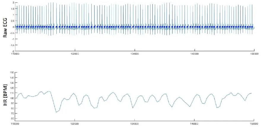
[image:1.595.76.519.365.589.2]1.i Illustrative plot of heart rate parsing
Figure S1 shows an illustrative plot of the data visualisations used to perform manual setting of the thresholds for ECG data parsing, and for post hoc checking of the accuracy of the results.
Supplementary Results
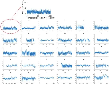
[image:2.595.75.518.198.547.2]2.i Heart rate parsing - separation into high and low frequency variability
Figure S2 shows the raw HR data collected during the experiment, rank ordered by mean HR obtained across the entire trial. This figure illustrates two clear parameters of variability in our data: first, they show consistent between-participant differences in mean HR, which is the focus of the analyses featured in the main text. Second, they show between-participant differences in heart rate variability. The analyses presented here examine this.
Figure S3: Illustration of two datasets from participants showing high and low Respiratory Sinus Arrhythmia (RSA). Plots a), b) and c) show data from a participant showing high RSA. a) raw time series of HR fluctuations over time (4 minute data sample); b) Poincaré plot showing HR at time t on x-axis and HR at time t+1 (the heart beat immediately following) on y-axis; c) Fourier plot showing a peak frequency at c.0.35Hz (corresponding to the respiration cycle). Plots d), e) and f) show identical plots from another participant showing low RSA. d) raw time series of HR fluctuations over time; e) Poincaré plot; f) Fourier plot showing a no clear peak in activity with the respiration cycle.
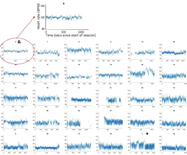
Figure S4: Raw HR data, rank ordered by RMSSD from lowest variability (top-left) to highest variability (bottom-right). The numbers above the plots show the participant number. The ‘high RSA’ sample illustrated in Figure S2 is highlighted with a * (bottom right on this plot). The ‘low RSA’ illustrated in Figure S2 is highlighted with a & (top left on this plot).
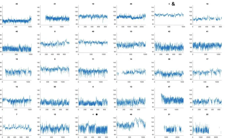
Figure S5: Raw HR data, rank ordered by RMSSD_low from lowest variability (top-left) to highest variability (bottom-right). The numbers above the plots show the participant number. As in Figure S4, the x axis shows the time (in seconds since the start of the session), and the y axis shows heart rate in beats per minute. The ‘high RSA’ sample illustrated in Figure S3 is highlighted with a * (bottom right on this plot). The ‘low RSA’ illustrated in Figure S3 is highlighted with a & (top left on this plot). Of note, and although low-frequency variability is often discussed in the literature as an index of sympathetic nervous system, the rank orderings of these datasets is quite similar between this plot and Figure S4. This point is discussed further in the Discussion in the main text.
In addition we also calculated the HF/LF ratio, which is sometimes thought to index sympatho-vagal balance (Berntson et al., 1997; although see Billman, 2013; Porges, 2007). This was calculated by dividing the low- and the high-frequency variability. A strong negative relationship was observed between HF/LF ratio and mean HR (29)=-.68, p<.001, suggesting that a higher ratio of HF to LF activity associates with lower HR.
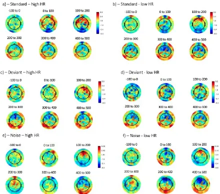
2.ii Topoplots in 100ms bins
Figure S6: topoplots for responses to all trials, split by the participants’ mean HR across the entire testing session and binned into 100 ms time intervals. The figure above each time plot indicates the mean time of each bin, in ms, relative to stimulus onset. The colour bar indicates the voltage, in V. a) Standard - high HR group; b) Standard - low HR group; c) Deviant – high HR group; d) Deviant – low HR group; e) Noise – high HR group; f) Noise – low HR group.
2.iii Relationship of high and low frequency variability to ERP responses.
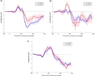
RMSSD showed a marginally non-significant relationship with N250 Standard amplitude (20)=-.43, p=.051, such that higher variability was associated with larger ERP amplitudes (Figure S8a). Figure S9 shows the averaged ERP responses, subdivided by high/low RMSSD. The results are highly similar to those obtained when results are subdivided by high/low mean HR (Figures 2c, 4c, 5c).
Relationships of the variability measures to P150 Deviant responses were also consistent with those reported in the main text, with comparable but marginally smaller effect sizes (Figure S8d-f). Overall, the relationships observed between HR variability and the ERP responses were as predicted based on the relationships between mean HR and ERP responses shown in the main text, and between mean HR and HR variability shown in the Figure S7.
Figure S8: a) scatterplot showing the relationship between RMSSD and N250 Standard amplitude; b) scatterplot showing the relationship between RMSSD_Low and N250 Standard amplitude; c) scatterplot showing the relationship between HF/LF ratio and N250 Standard amplitude; d) scatterplot showing the relationship between RMSSD and P150 Deviant amplitude; e) scatterplot showing the relationship between RMSSD_Low and P150 Deviant amplitude; f) scatterplot showing the relationship between HF/LF ratio and P150 Deviant amplitude.
[image:8.595.78.517.75.346.2] [image:8.595.74.390.466.719.2]2.iv Description of Ex-Gaussian Response Distribution fitting
A number of different distributions could have been used for this purpose, since the aim was not to find the best-fit but to compare parameters between distributions; the ex-Gaussian was selected as generally suitable given the shape of the data, although other distributions such as the gamma, lognormal or inverse Gaussian, could have been used instead (Johnson, Kotz, & Balakrishnan, 1994). The three components of the ex-Gaussian distribution describe, respectively, , the mode of the Gaussian component of the distribution; , the variance of the Gaussian component; and , the exponential (similar to the skewedness) (Lacouture & Cousineau, 2008).
For Standard Trials, results suggested that (mode of the Gaussian) was similar between the distributions: 87.3 for high HR and 88.5 for low HR. (variance of the Gaussian) was, however, markedly higher for the high HR group (14.8) than the low HR group (11.8). (exponential component) was also higher for the high HR group (0.43) than the low HR group (0.34). These results suggest that the modal responses are similar across the two populations, but that both components of response variability were larger in the high HR group.
For Deviant Trials, results suggested that (mode of the Gaussian) was again similar between the distributions – 98.4 for high HR and 99.1 for low HR. (variance of the Gaussian) was similar between the high and low HR groups: 7.6 for high HR and 8.1 for low HR. (exponential component) was markedly higher for the high HR group (10.9) than the low HR group (6.4). These results suggest that, whereas the modal responses were again similar between the two groups (shown by the similar components), the high HR group showed a sub-group of trials with a high response amplitude, manifesting as an increased (exponential component).
2.v Analysis examining within-participant changes in heart rate
The analyses presented in the main text examine between-participant differences based on mean HR recorded across the entire testing session. In addition, we wished to examine whether similar patterns could be identified when we examined within-participant variability – i.e. fluctuations in HR within a particular individual, within a testing session. Our analyses focused on the N250 component for Standard trials, and the P150/P3a component for Deviant trials, where significant group differences had been observed when examining between-participant differences in Analysis 1.
The results are shown in Figures S10b and S10c. For these plots, the individual datapoints show the average ERP amplitudes recorded for high HR (x-axis) and low HR (y-axis) trials. Figure S10b shows the Standard N250 amplitudes; a position above the 1:1 equivalence line indicates that, for that participant, the high HR trials showed higher amplitude (less negative) responses. Figure S10c shows the Deviant P150/P3a amplitudes; a position above the 1:1 line indicates that, for that participant, the high HR trials showed higher amplitude (more positive) responses. Paired-sample t-tests were conducted to compare amplitudes observed on high and low HR trials. Because both effects observed were directionally consistent with our predictions based on Analysis 1, one-tailed hypotheses were used. Significantly lower-amplitude N250 responses to Standard were observed during the high HR trials t(20)=1.8, p=.047. Results for the P150/P3a Deviant analysis (Figure 7c) include a clear outlier, more than 2 IQR from the mean. After this outlier was removed the results suggested that, although the effect observed was directionally consistent with our predictions, the result was not significant t(19)=.99 p=.17. The reason for this non-significant result is likely due to the lower sample size for this analysis (60 deviant trials per participant vs 280 standard trials).
trials, subdivided by mean HR at the time of the trial. X-axis shows the amplitude for high HR trials and y-axis shows the amplitude for low HR trials. The dashed line shows the 1:1 equivalence line: a position above this line indicates that, for that participant, the average amplitude for high HR trials was higher than for low HR trials.
Supplementary References
Berntson, G. G., Thomas Bigger, J., Eckberg, D. L., Grossman, P., Kaufmann, P. G., Malik, M., . . . Stone, P. H. (1997). Heart rate variability: origins, methods, and interpretive caveats. Psychophysiology, 34(6), 623-648.
Billman, G. E. (2013). The LF/HF ratio does not accurately measure cardiac sympatho-vagal balance. Frontiers in physiology, 4.
Bush, N. R., Alkon, A., Obradović, J., Stamperdahl, J., & Boyce, W. T. (2011). Differentiating challenge reactivity from psychomotor activity in studies of children’s
psychophysiology: Considerations for theory and measurement. Journal of Experimental Child Psychology, 110(1), 62-79.
Cacioppo, J. T., Tassinary, L. G., & Berntson, G. G. (2000). Handbook of Psychophysiology (2nd ed.): Cambridge University Press, Cambridge, UK.
Johnson, N. L., Kotz, S., & Balakrishnan, N. (1994). Continuous Univariate Probability Distributions,(Vol. 1): John Wiley & Sons Inc., NY.
Kushnerenko, E., Ceponiene, R., Balan, P., Fellman, V., & Näätänen, R. (2002). Maturation of the auditory change detection response in infants: a longitudinal ERP study.
NeuroReport, 13(15), 1843-1848.
Lacouture, Y., & Cousineau, D. (2008). How to use MATLAB to fit the ex-Gaussian and other probability functions to a distribution of response times. Tutorials in Quantitative Methods for Psychology, 4(1), 35-45.
Porges, S. W. (1995). Cardiac vagal tone: a physiological index of stress. Neurosci Biobehav Rev, 19(2), 225-233.
Porges, S. W. (2007). The polyvagal perspective. Biological Psychology, 74(2), 116-143. doi:10.1016/j.biopsycho.2006.06.009