i
Wave Propagation and Scour Failure of Coastal Structures
due to Tsunamis
Adewale Olusola Abimbola
A thesis submitted in partial fulfilment of the requirements of the
University of East London for the degree of Doctor of Philosophy
ii
Abstract
The extensive research on the influence of sea dike geometry on tsunami-induced scour indicates the necessity for a suitable model that can forecast the scour depth behind coastal structures and thus minimize the damaging effect of a high category tsunami occurrence. Current attempts to study this phenomenon have not gained worldwide acceptance and have been limited to unproven analytical methods, and either laboratory or numerical methods. These indicate the need for a verifiable predictive expression that links both the sediment characteristics and coastal defence geometry.
A comprehensive laboratory experiment was conducted to better understand the propagation mechanism of tsunami waves around four varying dikes sizes; two of which were modelled after dikes in Iwanuma and Soma cities in Japan that were affected by the 2011 Great Eastern Japan Earthquake and Tsunami. This investigation contributed to the understanding of the influence of dike dimensions on the flow variables. Afterwards, the mechanism of the induced local scour at the landward region was studied in detail because of the destructive impact it could have on the stability of the structures. These led to the development of a predictive scour model, from which a tsunami-induced scour resilient structure can be proposed. Also, using the particle size analysis, the median grain size and permeability properties of the sediment grain were determined and used to form the boundary condition of the expression.
The two-dimensional CFD analyses of the wave propagation and associated induced scour were investigated using ANSYS Fluent software package and sedFoam-2.0 solver respectively, and the results validated against the laboratory data showed good agreement. The Reynolds-Averaged Navier-Stokes (RANS) modelling approach with Realizable k-ε turbulence model and scalable wall function for wall modelling were employed for the wave flow, while turbulence-averaged Eulerian two-phase flow equations with the kinetic theory of granular flows for intergranular stress models and a k-ε turbulence model were used for the numerical implementation of the sediment scour.
iii
Title page i
Abstract ii
Table of Contents iii
List of Figures vii
List of Tables xiii
Nomenclature xv
Abbreviations xxi
Acknowledgements xxiii
Dedication xxiv
1 Introduction 1
1.1 Background of the Study 3
1.2 Aim and Objectives of the Study 4
1.3 The Scope of the Study 5
1.4 Outline of Thesis 5
2 Literature Review 7
2.1 Introduction 7
2.2 Water Wave Mechanics 7
2.3 Background of Tsunami studies 10
2.3.1 Tsunami 10
2.3.2 Experimental studies 11
2.3.3 Numerical studies 13
2.4 Flooding and Tsunami Mitigation Measures for Resilient Coastal Dike in Japan 14
2.5 Early History and Development of Numerical Simulation 19
2.6 Computational Fluid Dynamics Theory 21
2.6.1 Navier-Stokes equations 22
2.6.2 Reynolds-Averaged Navier-Stokes equations 23
iv
2.6.3.1 Standard k -є model 27
2.6.3.2 Realizable k -є model 29
2.6.4 The Volume of fluid method 30
2.6.5 Near-wall modelling 31
2.6.6 Wall functions 31
2.6.6.1 Standard wall functions 33
2.6.6.2 Scalable wall functions 35
2.7 Sediment Transport Mechanisms 35
2.7.1 Modes of sediment transport 35
2.7.2 Sediment transport modelling 36
2.7.2.1 Empirical bed load transport equations 39
2.7.2.2 Two-phase equation by Cheng and Hsu (2014) 44
2.7.2.3 Sediment transport model by Zhang and Shi (2016) 46
2.8 Summary 47
3 Tsunami Wave Propagation over Sea Dikes 48
3.1 Introduction 48
3.2 Laboratory Experiments 50
3.3 Tsunami Wave Flow over Sea Dike 54
3.3.1 Velocity distributions 54
3.3.2 The configuration of a pressure analog input measurement 60 3.3.3 Total tsunami wave pressure 61
3.3.3.1 Model A 62
3.3.3.2 Model B 62
3.3.3.3 Model C 63
3.3.3.4 Model D 63
3.3.4 Overflowing Wave pressure 68
v
4 Tsunami Induced Scour Profile on Erodible Boundaries 72
4.1 Introduction 72
4.2 Experimental Work 74
4.3 Scour Profile Characteristics 78
4.4 Scour Occurrence Validation with Shields parameter 84
4.5 Representative Scour Depth Predictive Model 87
4.6 Proposed Sea Dike Section to Resist Landward Toe Scour 92
4.7 Conclusions 94
5 Numerical Simulation of Tsunami Waves 96
5.1 Introduction 96
5.2 Numerical Investigation of Dam Break Flow – Two-phase Flow 99
5.2.1 Geometric setup and mesh generation 99
5.2.2 ANSYS Fluent setup 102
5.2.3 Total tsunami wave pressure 108
5.2.3.1 Model A 108
5.2.3.2 Model B 109
5.2.3.3 Model C 109
5.2.3.4 Model D 110
5.2.4 Velocity distributions at the landward region 119
5.2.5 Comparison between the numerical simulation and laboratory experiment 128
5.3 Numerical Methodology of Dam Break Flow - Comparison using ANSYS Fluent 129
5.3.1 Introduction 129
5.3.2 Computational setup 131
5.3.3 Results and discussion 132
5.4 Conclusions 134
6 Numerical Simulation of Tsunami-induced Sediment Scour 136
6.1 Introduction 136
6.2 SedFoam-2.0 Model- Two-phase Flow Solver 139
6.2.1 The governing equations 139
vi
6.2.3 Kinetic theory model 140
6.2.4 Model setup, initial and boundary conditions and mesh generation 141
6.2.4.1 Logarithmic velocity distribution 145
6.2.4.2 The shear stress at bottom-wall 145
6.2.5 Solution procedure 150
6.3 Scour Profile Characteristics 152
6.4 Comparison between the Numerical Simulation and Laboratory Experiment 160
6.5 Conclusions 162
7 Conclusions and recommendations 163
7.1 Conclusions 163
7.2 Recommendations 167
References 169
Bibliography 184
vii
List of Figures
Figure 1.1. Examples of damages caused by the 2011 Great Eastern Japan
Earthquake and Tsunami (Jayaratne et al., 2013). 2
Figure 1.2. Representation of the predictive model parameters. 4
Figure 2.1. Characteristics of linear water wave. 9
Figure 2.2. Phases of the evolution of a typical seismic generated tsunami from source to shore (Rossetto et al., 2011). 13
Figure 2.3. Parts of a dike (Japan International Cooperation Agency, 2010). 15
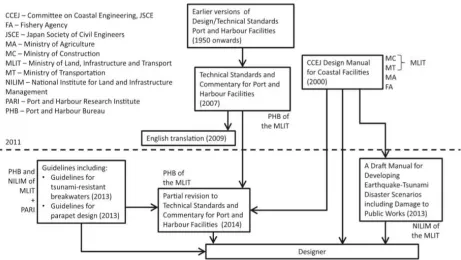
Figure 2.4. Evolution of official Japanese design guidelines following the 2011 Great Eastern Japan Earthquake (Raby et al., 2015). 17
Figure 2.5. Integration of trees with coastal dike (Torii, 2014). 17
Figure 2.6. Proposed resilient structure for coastal dike (Kato et al., 2012). 19
Figure 2.7. Variation of a velocity component, u, in turbulent flow (Cengel and Cimbala, 2014). 23
Figure 2.8. Near-wall cell (Craft, 2011). 32
Figure 2.9. Subdivisions of the near-wall region (Salim and Cheah, 2009). 33
Figure 2.10. The near-wall nodes (Launder and Spalding, 1974). 33
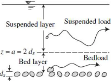
Figure 2.11. Bed load and suspended load (Julien, 2010). 36
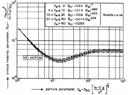
Figure 2.12. Initiation of motion according to Shields (Van Rijn, 1984). 40
Figure 2.13. Bed-load motion at equilibrium (Chanson, 1999). 43
Figure 3.1 Front view of hydraulic flume channel. 51
Figure 3.2. The layout of hydraulic flume (Not to scale). 51
Figure 3.3. Location of pressure sensors. 52
viii
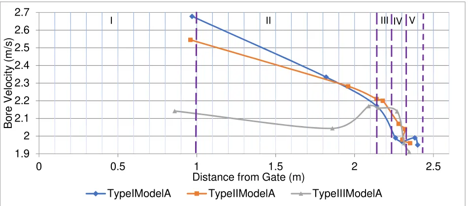
Figure 3.5. Section classification of the hydraulic flume. 56
Figure 3.6. Velocity distribution in the hydraulic flume. 58
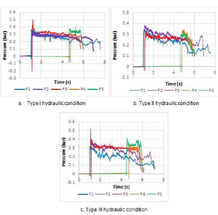
Figure 3.7. Total wave pressure distribution in Model A under various hydraulic conditions. 64
Figure 3.8. Total wave pressure distribution in Model B under various hydraulic conditions. 65
Figure 3.9. Total wave pressure distribution in Model C under various hydraulic conditions. 66
Figure 3.10. Total wave pressure distribution in Model D under various hydraulic conditions. 67
Figure 3.11. The relationship between overflowing wave pressure and flow quantities from experimental (Exp.) studies. 68
Figure 4.1. Schematic sketch of the experimental set-up at UEL. 74
Figure 4.2. Front view of the representation of experimental set-up. 75
Figure 4.3. Grain size distribution curve. 75
Figure 4.4. Point gauge (manually operated) for measuring scour profile. 77
Figure 4.5. Snapshot of model C scour experiments. 78
Figure 4.6. Non-dimensional scour profiles of sea dike models (Models A, B, C, and D). 80
Figure 4.7. Scour development profile (Models A, B, C, and D). 83
Figure 4.8. The non-dimensional relationship between the average horizontal location of maximum scour depth and angle of seaward slope. 83
Figure 4.9. The non-dimensional relationship between the average horizontal location of maximum scour depth and angle of landward slope. 84
ix
Figure 4.11. A comparison between the Hjulstrom curve and the shields curve
(Miedema, 2008). 86
Figure 4.12. Mathematical modelling construction steps (Giordano et al., 2009). 87 Figure 4.13. The relationship between relative scour depth and maximum overflowing wave pressure. 89
Figure 4.14. Design recommendation for a resilient coastal dike structure to mitigate the landward toe scour. 93
Figure 5.1. ANSYS Workbench project tab. 100
Figure 5.2. Geometry generation using DesignModeler. 100
Figure 5.3. Mesh generation using meshing application. 101
Figure 5.4. Different parts for boundary condition set up in Fluent. 101
Figure 5.5. Quality metrics of mesh. 102
Figure 5.6. Multiphase model set-up. 103
Figure 5.7. The solution method for setting up physics of flow. 106
Figure 5.8. The volume fraction of the phases during flow over the sea dike model. 107
Figure 5.9. The volume fraction of the phases after flow over the sea dike model. 107
Figure 5.10. Solution procedure flowchart in ANSYS Workbench 18.1. 108
Figure 5.11. Total wave pressure distribution in Model A under various hydraulic conditions. 112
Figure 5.12. Total wave pressure distribution in Model B under various hydraulic conditions. 114
x
Figure 5.14. Total wave pressure distribution in Model D under various hydraulic
conditions. 118
Figure 5.15. maximum scour velocity comparison between numerical and laboratory
data. 119
Figure 5.16. Velocity distribution behind Model A under various
hydraulic conditions. 121
Figure 5.17. Velocity distribution behind Model B under various
hydraulic conditions. 123
Figure 5.18. Velocity distribution behind Model C under various
hydraulic conditions. 125
Figure 5.19. Velocity distribution behind Model D under
various hydraulic conditions. 127 Figure 5.20. The relationship between overflowing wave pressure and flow quantities from experimental (Exp.) and numerical (Num.) simulation. 128 Figure 5.21. A side view of hydraulic flume with locations of water level measuring positions (left) and a front view showing the locations of pressure sensors at the impact wall downstream the dam (right).
Dimensions in millimetres(Lobovsky et al., 2014). 130 Figure 5.22. Different zones for boundary condition setup in Fluent (Zone 1: Free surface, Zone 2: Inlet, Zone 3: Right wall, Zone 4: Bottom wall, Zone 5: Left wall). 131 Figure 5.23. H = 300 mm; free surface flow at 183 and 263 ms. 132 Figure 5.24. Free surface profile and upstream wave at the instant of complete dam gate removal. H = 300 mm (left), H = 600 mm (right). 133 Figure 5.25. Numerical simulation value of dynamic pressure at sensors 1 – 4
xi
Figure 6.2. Fine grid size (Block 0 cell size is the sediment region, and Block 1 cell
size is the water region). 143
Figure 6.3. Schematics of the landward region (refer to the boundary and zone columns in Table 6.1). 144
Figure 6.4 Shear stress distribution at bottom-wall (Zone 2) of Model A under various hydraulic conditions. 146
Figure 6.5 Shear stress distribution at bottom-wall (Zone 2) of Model B under various hydraulic conditions. 147
Figure 6.6. Shear stress distribution at bottom-wall (Zone 2) of Model C under various hydraulic conditions. 148
Figure 6.7. Shear stress distribution at bottom-wall (Zone 2) of Model D under various hydraulic conditions. 149
Figure 6.8. Using logarithmic velocity distribution to link two CFD tools for tsunami-induced scour process. 150
Figure 6.9. Solution procedure flowchart in sedFoam-2.0 (Adapted from Cheng and Hsu, 2014; Chauchat et al. 2017). 151
Figure 6.10. Coarse grid size (Block 0 cell size is the sediment region, and Block 1 cell size is the water region). 153
Figure 6.11. Stability of sediment concentration calculation at 4 s by using a fine grid size. 153
Figure 6.12. Instability of sediment concentration calculation at 0.5 s by using a coarse grid size. 154
Figure 6.13. Scour profile of Model A under various hydraulic conditions. 156
Figure 6.14. Scour profile of Model B under various hydraulic conditions. 157
Figure 6.15. Scour profile of Model C under various hydraulic conditions. 158
xii
Figure 6.17. The relationship between relative scour depth and impact overflowing
xiii
List of Tables
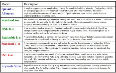
Table 2.1. Wave classification (Anderson & Frigaard, 2008). 9 Table 2.2. Crest width of a dike (Japan International Cooperation Agency, 2010). 15 Table 2.3. Minimum required freeboard (Japan International Cooperation Agency, 2010). 16 Table 2.4. RANS turbulence model description (ANSYS, 2006). 26 Table 2.5. RANS turbulence model behaviour and usage (ANSYS, 2006). 27 Table 2.6. Comparison of Sediment transport model (Hanna, 2014). 37 Table 2.7. Empirical and semi-empirical correlations of bed load transport (Chanson,
1999). 42
Table 2.8. Bed-load transport rate calculations (Chanson, 1999). 44 Table 3.1. Hydraulic conditions used in experiments. 52
Table 3.2. Coastal dike model geometry. 53
Table 3.3: Bore velocity readings for model dikes (Models A, B, C, and D). 58 Table 3.4. Average Error of the observed data from the overflowing wave pressure
model. 69
Table 4.1. Root mean square error of the field survey data compared with the scour
predictive model. 90
Table 4.2. Root mean square error of the experimental data compared with the scour
predictive model. 91
xiv
Table 5.3. Comparison of numerical and experimental average Errors of the observed data from the overflowing wave pressure model. 129 Table 5.4. Boundary conditions for geometry parts in Fluent. 131 Table 6.1. Summary of boundary condition in the 2D sediment scour experimental configuration: zG = zeroGradient, fV = fixedValue, dM = directionMixed, fFP = FixedFluxPressure and hp = hydrostatic pressure. 144 Table 6.2. Root mean square error of the numerical data compared with the scour
xv
Nomenclature
Roman Symbols
Speed of sound
a Wave amplitude
A Area of the cross section
C Correction factor C Wave celerity
Cc Coefficient of curvature Cu Uniformity coefficient
Ch ́zy-coefficient related to surface or grain roughness of the sediment bed
s Mean sediment concentration
, , Empirical coefficients in the k-εModel , Empirical coefficients in the k-εModel dM directionMixed
D Water depth
Ds Representative/maximum scour depth
D10 Diameter just larger than the diameters of 10% of the soil grain D50 Average sediment size
D60 Diameter just larger than the diameters of 60% of the soil grain D90 Diameter just larger than the diameters of 90% of the soil grain
∗ Dimensionless grain diameter/Bonneville parameter D/Dt Substantial derivative in Cartesian coordinates E Average error
E Empirical constant; the function of wall roughness
f Body force
External force that drives the flow fFP FixedFluxPressure
fV fixedValue
Gravitational vector component in the ith direction g Gravitational acceleration
h Inundation height.
xvi
hd Downstream water depth ho Initial bed depth
hp Hydrostatic pressure
hu Upstream water depth
Hd2 Height of structure measured on the landward side i Unit vector along the x-axis
I Turbulent intensity
j Unit vector along the y-axis Fluid-particle interaction term k Unit vector along the z-axis
K Coefficient of soil permeability Drag parameter
Turbulent kinetic energy
Turbulence kinetic energy at the near-wall node P
Nikuradse roughness length/equivalent roughness of the bed Angular wave number
L Wavelength
Lm Model length
Lms Horizontal location of representative/maximum scour depth
Lp Prototype length
LR Length ratio between prototype and model
Ls Scour length
/ Interphase momentum transfer term between sediment and fluid phase Turbulent Mach number
! " mass transfer from phase p to q !" mass transfer from phase q to p
n Porosity
N Total number of data
Nx Grid length in the x-direction Ny Grid length in the y-direction Nz Grid length in the z-direction P Wetted parameter
xvii Pm Model wave pressure
Pom Maximum Overflowing Pressure Pp Prototype wave pressure
%& Particle pressure %'& Particle normal stress
% Fluid pressure
#( Production of % Particle pressure P1 Pressure sensor one P2 Pressure sensor two P3 Pressure sensor three P4 Pressure sensor four P5 Pressure sensor five
Pr Prandtl number
+∗ Dimensionless bed flux +$ Bed-load transport
qbi Bed load sediment transport rate at i direction +, Granular temperature flux
+-/+ Bed-load transport rate per unit width Re Reynolds number
R2 Coefficient of determinant /$ Hydraulic radius
Rd Relative density s Specific gravity
S Modulus of the mean rate-of-strain tensor Sij Strain rate tensor
01 Source term
, Deviatoric part of strain rate tensor for sediment phase Inverse of Schmidt number
t Time
23 Turbulent drag parameter T Transport stage parameter
xviii
Tm model time
Tp Prototype time
τij Total shear stress/ Reynolds stress tensor 4 Bottom wall shear stress
u Velocity in the x-direction
5 Mean velocity of the fluid at the near-wall node P
67 Steady/mean velocity term 6 Fluctuating velocity term
6 ∗ Bed shear velocity related to grains 6 /6 $ 8 velocity component of the fluid phase 6 /6& 8 velocity component of the sediment phase 6∗ Shear velocity
6∗,9: Shields critical bed shear velocity U* Dimensionless velocity
Ucr Critical average velocity above the bed
v Velocity in the y-direction V Velocity component ;$ Fluid viscosity
<3 Maximum velocity over the crest measured at the landward region Vp Prototype velocity
< Average sediment velocity in the bed load layer ; $ Turbulent viscosity
w Velocity in the z-direction
x Streamwise direction
=> Dimensionless maximum overflowing wave pressure
y Spanwise direction ? Observed data
@ Distance from point P to the wall
YM Dilation dissipation
?> Model data
y+/y* Dimensionless distance from the wall
xix
AB Constant of integration in the rough wall log-law
Greek Symbols
α Angle of slope of the bed
C Particle volumetric concentration
αi Dimensionless initial downstream water depth β Fluid volumetric concentration
D Thermal expansion coefficient
E Energy dissipation rate due to an inelastic collision ∆x Grid length in the x-direction
∆y Grid length in the y-direction ∆z Grid length in the z-direction
F Average saltation height measured perpendicular to the bed F, Kronecker delta
∂ Partial derivative ε Turbulent dissipation
η Water surface elevation
H Angle of landward slope of the coastal dike H/I∗ Dimensionless shear stress/Shields parameter H9:/I∗9 Critical Shields parameter
H9:B Critical shields number at the horizontal bed H /φ Angle of repose of the sediment
Turbulent length scale ҝ Von K rm ́n constant L Scour fitted coefficient L Friction coefficient
xx P Density of sediment
I Viscous stress
I Shear stress at i direction I,$ Fluid shear stress
I, /I,& Particle stress I- Bed shear stress
I Shear stress on the wall
ɸ Sediment volumetric concentration RST
7777 Mean rate-of-rotation tensor observed in a rotating reference frame R Computational domain
ω Angular frequency
ω Specific rate of dissipation U( Angular velocity
Other Symbols
Θ Granular temperature
∇ Vector operator in the Cartesian coordinates ∇2 Laplacian operator in Cartesian coordinate ( )
xxi
Abbreviations
1D One-dimensional
IDV One-dimensional Vertical 2-D Two Dimensional
3-D Three Dimensional
CFD Computational Fluid Dynamics
COMCOT Cornell Multi-grid Coupled Tsunami Model DAQ Data Acquisition
DART Deep-ocean Assessment and Reporting of Tsunamis
DBW Dam Break Wave
DNS Direct Numerical Simulation FDM Finite Difference Method FEM Finite Element Method
FPS Frame Per Seconds
FVM Finite Volume Method GUI Graphical User Interface LBM Lattice Boltzmann Method LES Large Eddy Simulation MAC Marker-and-Cell
MANIAC Mathematical and Numerical Integrator and Computer MWL Mean Water Level
MOST Method of Splitting Tsunami MRS Mean Reynolds-Stress Closure MTE Mean Turbulent Energy
MVF Mean-Velocity Field Closure MWL Mean Water Level
NOAA National Oceanic and Atmospheric Administration NCTR NOAA Center for Tsunami Research
NI National Instrument
PISO Pressure-Implicit with Splitting of Operators PIV Particle Image Velocimetry
xxii PTV Particle Tracking Velocimetry RANS Reynolds-Averaged Navier-Stokes RMSE Root Mean Square Error
RNG Re-Normalisation Group
SGS Subgrid Scale
SIFT Short-term Inundation Forecasting for Tsunamis SLIC Simple Line Interface Calculation
SPH Smoothed Particle Hydrodynamics SST Shear Stress Transport
SW Well-graded sandy soil SWL Still Water Level
TDMS Technical Data Management Streaming TIME Tsunami Inundation Modelling Exchange UDF User-Defined Function
USCS Unified Soil Classification System
VI Virtual Instrument
xxiii
Acknowledgements
My most profound appreciation to my Director of Studies, Dr Ravindra Jayaratne, and supervisor, Dr Ali Abbas, for their continuous support and guidance. I am deeply indebted to Dr Ravindra Jayaratne, for his patience, valuable insight and direction. He always inspired me to approach problems from a new perspective when stagnated. I am much inspired by his attitude to novelty and high quality of research. He provided work reference for me when needed and the opportunity to lecture within the University for three years. I would like to thank Dr Ali Abbas for his valuable suggestions which improved the approach to my methodology and interpretation of results.
My sincere gratitude for the huge input of Mr Neil Goodin and Mr Joe Kennedy, the senior technicians, who helped set up and provided training for the operations of the laboratory equipment and the fabrication of the models employed in the study. Also, I am grateful to Cheryl Wheeler for her computing help in setting up the required software for this project. I am thankful to Mrs Avinder Bhinder, Ms Charlotte Forbes and Mr Richard Bottoms for their administrative assistance during my study.
Dr Awan Nas Ruqiyabi made research methods a passion for doctoral students, not just a class or subject to teach. Her broad knowledge and guidance were helpful during the early period of my work. The lectures provided me the skills to adequately plan for the timely completion of my programme.
I owe thanks to Dr Laszlo Konozsy and Dr Zeeshan Rana at Cranfield University for their advice on multiphase flow and turbulence modelling. I am grateful to Dr Martin Marriott, Dr John Walsh and Dr Darion Grant for their contributions during the annual monitoring reviews. My gratitude to Prof Hassan Abdalla for the approval of my continuous professional development training, which helped broaden my knowledge of Computational Fluid Dynamics.
xxiv
Dedication
To my wife; Olori mi, Adenike, for her unwavering love and support to make this voyage a reality, without her endurance and continual encouragement, this work
could not have been completed.
To my son; the beginning of my strength, Oluwadamilare, for the warmth, smile, and joy he brings to my heart; his face continually reminding me of the sacrifice I must
make for his future.
To my parents and siblings for their continuous prayers, and support. Always bringing love so close, so familiar yet so sweet.
1
Chapter 1
Introduction
The giant strides that have been made recently in the study of a tsunami have been due to efforts to understand the complex phenomenon and mitigate the huge damages resulting from the event. These have led to the inclusion of the safety factors in building codes to cater for forces generated by tsunami bores, determination of tsunami impact overflowing pressure over coastal structures, development of different numerical models to comprehend the phenomenon and construction of various hard and soft engineering methods that are being employed to alleviate tsunami impact. Despite these, tsunami-induced scour around coastal structures, which caused the most significant damage in the 2011 Great Eastern Japan Earthquake and Tsunami (Fig. 1.1), has not been meticulously investigated while studies have only been limited to the investigation of scour processes around vertical cylinders and breakwaters, understanding of tsunami flow and the general failure patterns associated with coastal structures.
2
Figure 1.1. Examples of damages caused by the 2011 Great Eastern Japan Earthquake and Tsunami (Jayaratne et al., 2013).
The aftermath of the catastrophic damages showed the need for improved structurally resilient coastal defences to a high-level tsunami phenomenon, as comprehensive understanding scour mechanism and associated instability to coastal structures are not yet adequately understood. The high cost of protecting the long stretch of foundation necessitates the study of scour depth and length to assess the risk of such failure (Karim and Ali, 2000). The study of the characteristics of scour holes development behind coastal defences can improve the understanding of their structural stability.
In the past, the primary approach to studying tsunami flows was experimental, and the turbulence in the surf zone is still one of the most challenging natural problems to any researcher in hydrodynamics or fluid mechanics, but with the development of more advanced measuring technology and more advanced numerical models, this hydrodynamics can now be studied in much more detail (Thao, 2007). Mikami et al. (2014) employed Large Eddy Simulation (LES) model in their numerical experiments to study the hydraulic characteristics of overflowing tsunamis around coastal dikes (velocity and pressure fields) and concluded that the structural survival of a coastal dike could depend on a milder landward slope and the construction of obstructions like secondary dikes and coastal forests.
3
The results are then compared with the scour depth model predicted by Jayaratne et al. (2014). Also, a Reynolds-Averaged Navier-Stokes (RANS) turbulence model and a two-phase sediment transport model are employed to validate the laboratory findings numerically.
In this chapter, comprehensive background of the research, the aim and objectives of the study are provided. After that, the scope of the study is described, and the outline of the thesis presented.
1.1 Background of the Study
Kato et al. (2012) performed hydraulic model experiments and an extensive field survey along the coastlines of Amori and Chioba prefectures in Japan after the 2011 Tohoku tsunami and concluded that scouring at the leeward toe of the dikes was the dominant failure pattern. The experiment estimated that 49.2% of the eight failure patterns studied was because of scouring at the landward toe. It was against this backdrop that Abimbola (2013) and Jayaratne et al. (2014) employed mathematical modelling technique to develop a scour predictive model for a quasi-steady tsunami flow (Eq. 1 & Fig. 1.2) at University of East London. The model is based on results of field investigation carried out in Miyagi and Fukushima Prefectures of Japan, the maximum wave pressure formula developed by Mizutani and Imamura (2002 cited by Kato et al., 2007), and tsunami velocity model developed by Matsutomi et al. (2010). It applies to sediments with the coefficient of permeability (m/s), K, between 10-4 and 10-3.
YZ
[\]= L _ `%(−
b[\]
c√e f] ) g (1) where, is the representative scour depth (m), L is the scour coefficient (0.85), hi is the height of structure measured in leeward side (m), H is the angle of landward slope of coastal dike, and ℎis the inundation height (m).
ϰ
Figure 1.2. Representation of the Predictive Model Parameters.
1.2 Aim and Objectives of the Study
The primary aim of this research is to perform extensive small-scale laboratory experiments and numerical simulation to elucidate further the scour failure of coastal dikes due to tsunami wave attack. To meet the general aim of this research project, the study will focus on the following objectives:
• To develop a comprehensive experimental programme to study tsunami flow hydrodynamics and its associated hydro-sedimentary characteristics, to assess the extent of scour failure of coastal defences.
• To implement numerical methods to validate the experimental studies of tsunami propagation and tsunami-induced scour failure at the landward region of a coastal dike.
• To employ both laboratory and numerical data to improve the theoretical scour predictive model developed by Abimbola (2013).
• To use sediment transport theory to support evidence of the laboratory and numerical studies of tsunami-induced scour at the landward toe of the coastal dike.
5
1.3 The Scope of the Study
The above discussion reveals the need to investigate tsunami wave flow and its induced scour, either by experimental studies or numerical simulations. Thus, this study attempts to improve understanding of these processes.
Experimental works are employed to study tsunami propagation and scour over four sea dikes models, of which two were modelled after some of the prototypes that were substantially damaged in Iwanuma and Soma cities of Japan by the 2011 Great East Japan Earthquake and Tsunami (Jayaratne et al., 2013). The hydrodynamic study was carried out by adopting a two-phase flow model in Ansys Fluent 18.0 to simultaneously solve the flow in both air and water phases. Flow variable results were then adapted into a two-phase flow solver; SedFoam- 2.0, to study the scour process. The experimental and numerical simulations were carried out to validate tsunami field results and results from existing tsunami studies.
1.4 Outline of Thesis
The seven parts of this thesis begin with the introduction in Chapter 1. The other chapters are organised as follows:
Chapter 2 highlights the literature review of the study. The different classifications of water waves are presented, and this leads to the background studies of tsunami waves, including the past occurrences of the phenomenon and its damaging effects on humans and environment. Different recent experimental and numerical studies are detailed to reveal development in tsunami studies. An initial introduction to early history and development of numerical simulation is also included. Important descriptions of the basic theory of Computational Fluid Dynamics (CFD) and sediment transport mechanism that relate to this study.
6
In Chapter 4, the experimental studies of tsunami-induced scour profile on erodible boundaries are presented. Scour profiles characteristics derived from measurements are shown, including the validation of the possibility of scouring occurrence using Shields parameter. The steps for the derivation of the representative scour depth predictive model were shown, and the section for a coastal dike capable of resisting landward toe scour was proposed.
In Chapter 5, the RANS study of two-dimensional tsunami waves is discussed, and numerical validation of experimental study of tsunami wave propagation is presented. The boundary conditions, computational domain, and the solution procedure are also described. The various pressure distributions over the four model sea dikes are presented, and detailed analyses are carried out with appropriate conclusions provided.
Chapter 6 provides a numerical validation of experimental studies of tsunami-induced scour behind the sea dike models. The solver set-up, boundary conditions, computational domain, and the solution procedure are also described. The computer simulation results of the scour process for the two-phase flow as performed in SedFoam- 2.0 are presented.
7
Chapter 2
Literature Review
2.1 Introduction
The damaging impact of tsunami wave and the importance of a comprehensive understanding of the flow characteristics to help mitigate its detrimental human and socio-economic effect have been briefly discussed in the previous chapter. Over the years coastal engineers have devoted huge effort and capital in the design of robust structures against different wave classification. However, the initial literature review revealed that only very few studies had been conducted about proposing resilient structures against tsunami-induced scour in the leeward region of coastal structures. Early studies have primarily used physical models and mathematical models to understand the behaviour of several wave characteristics. The advent of faster computers in recent years have accelerated the development of turbulence and sediment transport models, to understand the fluctuating characteristics of turbulent flows and kinematic interaction between sediment particles.
In this review, aspect relating to water wave mechanics and background of experimental and numerical tsunami studies are discussed. The flooding and tsunami prevention measures for resilient coastal dike in Japan, early history and development of numerical simulation, basic Computational Fluid Dynamics (CFD) theories, and sediment transport mechanism as they pertain to the methodologies used in further chapters of this research are presented.
2.2 Water Wave Mechanics
ϴ
The complexity and various water wave motions make its classification difficult. According to Mader (2004), oscillatory and translatory waves are the two kinds of water waves based on the transportation of fluid. In translatory waves, transport of fluid occurs in the direction of wave travel, while mass movement of fluid is absent in oscillatory waves. Some examples of a translatory wave include waves generated by the breaking of a dam, tidal bore or moving hydraulic jump, flood waves in rivers and solitary waves. An oscillatory wave can be progressive or standing. The harmonic wave which is defined by a sine or cosine curve is the simplest case of a progressive wave. A standing wave can be considered as the superposition of two waves of the same amplitude and period, but travelling in opposite directions.
Waves can also be grouped based on their frequency and method of generation (Andersen and Frigaard, 2007). The phenomenon presented in the first group (Table 2.1) is characterised by changes in Mean Water Level (MWL) and not commonly referred to as waves.
Wave is also classified based on the depth of the water. Physical observation of water wave reveals that its particles disappear with depth. Particles get more agitated as they approach the shore than in the open sea. This classification is based on the ratio of wave depth, D, to wavelength, L. A wave is classified as a deep-water wave or short wave if ୈ > 0.5, intermediate water waves if 0.05 < ୈ < 0.5, and shallow-water wave or long wave if ୈ < 0.05.
Figure 2.1 shows the characteristics of a linear wave, where L = ்ଶSమis the wavelength,
H is the wave height, a = ுଶ is the wave amplitude, D is the water depth referenced from the horizontal bed, @is the water surface elevation. Other important parameters are the wave celerity, C = ் , angular wave number, ܭ௪ = ଶS, and angular frequency,
9
Figure 2.1: Characteristics of linear water wave.
Table 2.1. Wave classification (Andersen and Frigaard, 2007).
Phenomenon Origin Period
Surges. Atmospheric pressure and wind. 1 - 30 days.
Tides. Gravity forces from the moon and the sun.
Approximately 12 and 24 hours.
Barometric wave. Air pressure. 1 - 20 hours.
Tsunami. Earthquake, submarine landslide or submerged volcano.
5 - 60 minutes.
Seiches (Water level fluctuations in bays and harbour basins).
Resonance of long period wave components.
1 - 30 minutes.
Surf boat, mean water level fluctuations at the coast.
Wave groups. 0.5 - 5 minutes.
Swells. Wave generated by a storm some
distance away.
less than 40 seconds. Wind generated waves. Wind shear on the water surface. less than 25
seconds. Still Water Level (SWL)
Direction of travel
x η (x, t)
Y Crest
H L
Trough D
a
10
It is known that water propagates as its particle moves in an oscillatory action, and the type of action depends on the depth of water. They move in a circular orbit in deep water, elliptical orbit in intermediate water and shallow water (Jayaratne, 2012). According to Kinsman (1965), for an oscillation to occur, there must be an equilibrium state, a disturbing force to disturb the equilibrium and a restoring force to re-establish the equilibrium. He further opined that gravity, surface tension, and Coriolis force are the three principal restoring forces associated with water wave propagation.
This subject of water wave classification would be needed as we focus more on tsunami wave in the following section.
2.3 Background of Tsunami Studies
2.3.1 Tsunami
‘Tidal wave’ and ‘seismic wave’ are two old imprecise terms that were generally referred to as tsunami because of the inaccurate understanding of its generation mechanisms. The former suggests the influence of movement of planetary bodies, while the latter only restricts its cause to an earthquake. Tsunami is a wave train generated by a vertical displacement of the water column. It is now acknowledged that this displacement can be generated by an earthquake, volcanic activity, meteorite impact, or landslide. The present study shall be limited to tsunami induced by seismic activity.
The National Oceanic and Atmospheric Administration, NOAA, on their website (http://www.ngdc.noaa.gov/hazard/tsu_db.shtml), provides details of tsunami events that date back to 2000 B.C in the Global Historical Tsunami Database. Recent tsunami occurrences; 2004 Indian Ocean Tsunami, 2010 and 2015 Chile Tsunami, 2011 Japan Tsunami, and 2013 Solomon Island Tsunami have led to the significant advances made theoretically, experimentally and in numerical studies to better understand the characteristics of tsunami.
11
tsunami can have a period in the range of five minutes to two hours as opposed to wind-generated waves of five to thirty seconds period. As a shallow water wave, its speed, acceleration due to gravity and water depth relationship, C =b p, reveal that tsunami speed will reduce on approach to shore. The high speed coupled with low amplitude make tsunami virtually undetected by human eyes in the deep ocean. A tsunami can travel great distance because the rate at which it loses its energy is inversely related to its wavelength. Since a tsunami has a very large wavelength, it will lose little energy as it propagates. A tsunami will travel at high speeds with little loss of energy in very deep water because the change of total energy of a tsunami is constant.
According to Dias and Dutykh (2006), ‘the life of tsunami is usually divided into three phases: the generation (tsunami source), the propagation and the inundation.’ The most critical phase, inundation phase, which is associated with large amplitude change of the wave, depends significantly on the bottom bathymetry and the coastline type. The structural and human damages are mainly because of the inundation. The 2004 Indian Ocean Tsunami caused nearly 230,000 deaths and $10 billion in damage, the 2010 Chile Tsunami resulted in over 156 deaths, $30 billion damage, 2011 Japan Tsunami caused $220 billion and over 17,000 deaths, and the 2013 Solomon Island Tsunami caused 10 deaths, 14 injuries, with damage and destruction of more than 700 houses (NOAA, 2014).
2.3.2 Experimental Studies
In many hydraulic experimentations, solitary waves have been used as an approximate wave type for tsunami representation, but Rossetto et al., (2011) used a new approach of wave generation to recreate seismic generated tsunami waves in a laboratory. This new concept makes use of a wave generator capable of recreating scaled tsunami waves. The wave generator can be used to reproduce solitary waves and N-waves with large wavelength.
A theoretical solitary wave is described by Miles (1980 cited by Rossetto et al., 2011) as:
12
where, η is the surface elevation (m), ` is the horizontal coordinate, 2 is time (s), a is the wave amplitude (m), is the wave celerity (m/s), o is the wavelength (m), and sech is the hyperbolic secant function that defines the exponential behaviour of the wave in space and time.
Using a constant mass density, Le roux (2009) constructed a velocity-pressure; non-homogeneous Euler-like, model to discuss the formation of a tsunami wave. According to Mikami and Shibayama (2013), three types of method are used to generate a tsunami-like flow in a wave flume or numerical model - using a solitary wave, dam break method and a pump flow method. The 2011 Tohoku Earthquake and Tsunami gave rise to the widespread use of the pump flow method because of the ease of creating a prolonged overtopping flow, which the solitary wave method does not offer. Mizutani and Imamura (2001) discovered that four types of wave pressure are generated by a tsunami wave force acting on a coastal structure: dynamic, sustained, impact standing and overflowing. The hydraulic experiments revealed that the impact standing and overflowing pressures generated the largest wave forces and should be given significant consideration when designing a coastal structure. They observed that the collision between reflected and incident waves generated the impact standing wave pressure, while the wave impact on the back of the structure generated the overflowing wave pressure. The overflowing pressure formulas generated by the study was confirmed by Kato et al. (2007) in their large-scale experiment to evaluate tsunami wave force on coastal dike by taking into consideration the effects of wave transformation and dike slope.
13
Figure 2.2. Phases of the evolution of a typical seismic generated tsunami from source to shore (Rossetto et al., 2011).
2.3.3 Numerical Studies.
COMCOT (Cornell Multi-grid Coupled Tsunami Model) offers the possibility of simultaneously calculating tsunami inundation and tsunami propagation in deep oceans. A nested grid system is adapted to balance its efficiency and accuracy. In this system, a modified leap-frog finite difference method is used to solve the linear or nonlinear shallow water equations (Li et al., 2012; Wang, 2009; Wijetunge, 2009). TUNAMI-N2 model is based on the TUNAMI-N1 numerical code developed by Dr. Fumihiko Imamura of Tohoku University for the 1995 Tsunami Inundation Modelling Exchange (TIME) project. It was used to study tsunami propagation and its coastal amplification with different initial conditions. It was implemented to simulate tsunami propagation and run-up in Pacific, Atlantic and Indian Oceans, with emphasis around the Japanese, Caribbean, Russian and Mediterranean seas (Yalciner et al., 2004). It uses leap-frog finite difference scheme to discretize a set of nonlinear shallow water equations. A detailed description can be found in Imamura et al. (2006).
The TUNAMI-N2-NUS, a developed version of TUNAMI-N2 model, was developed by Dao and Tkalich (2007) for operational forecasting. It considers phenomena: sea bottom friction, dispersion, spherical curvature, astronomical tide and Coriolis force, which could affect tsunami dynamics.
ϭϰ
tsunami modelling from several observatory systems – seismic network, Deep-ocean Assessment and Reporting of Tsunamis (DART) and coastal tide gauges – to provide inundation forecast; tsunami arrival time and amplitudes and tsunami impact at specific coastal areas during an event (Titov et al., 2001). According to Gica et al. (2007), the system is more than an operational tool as it can also be used for hazard assessment studies by generating and studying different tsunami scenarios.
2.4 Flooding and Tsunami Mitigation Measures for Resilient
Coastal Dike in Japan
Dike is usually reconstructed natural ridge or artificial wall built along the banks of stream, river, lake or other bodies of water, primarily for regulation of water levels or flood prevention. Sea dike, also known as embankment, dike or levee, provides socioeconomic and environmental benefits. The benefits include:
• Protection of hinterland or coastal zones to generate revenue from tourism.
• Prevention of high damage cost as a result flooding caused by sea level rise.
• It can be restored quickly if damaged by flood, earthquake, tsunami or other disasters.
• Protection against high water pressure, wind current and storm surges to minimize adverse impacts.
• Its durability suggests that it can last for thousands of years if maintained adequately.
• It can be improved easily if the scale of flood control plan is to be increased.
ϭϱ
Figure 2.3. Parts of a dike (Japan International Cooperation Agency, 2010).
According to Japan International Cooperation Agency (2010), the technical standards and guidelines for sea dike include:
• The crest width of the dike shall be based on the design flood discharge in Table 2.2 and should be designed for multi-purpose use, such as for patrolling during floods and in the execution of emergency flood prevention works.
Table 2.2. Crest width of a dike (Japan International Cooperation Agency, 2010).
ϭϲ
• A berm width of at least 3 m shall be provided along the slope for stability, repair and maintenance purposes if the dike height is more than 5 m.
• Freeboard is the margin from the design flood level up to the elevation of the dike crest. It is designed based on the design flood discharge which shall not be less than the value given in Table 2.3.
Table 2.3. Minimum required freeboard (Japan International Cooperation Agency, 2010).
17
Figure 2.4. Evolution of official Japanese design guidelines following the 2011 Great Eastern Japan Earthquake (Raby et al., 2015).
[image:41.595.77.538.74.334.2]In 2013, the Coastal Management Review Committee released proposals for coastal management. These were to update the 1999 Seacoast Law, by including lessons from the 2011 Great Eastern Japan Earthquake and the gradual deterioration of coastal protection infrastructure (Suwa and Watanabe, 2014). A disaster mitigation measure of integrating green embankment with resilient coastal dikes was proposed, to reduce inland flood heights and delay wave overtopping for safe evacuation (Fig. 2.5). This system can be sustained for a thousand year through maintenance of the structural measure.
18
Two levels of a tsunami were established following the 2011 Great Eastern Japan Earthquake. Level 1 tsunami is more frequent with a return period of several decades to few hundred years and has lower inundation height between 7 and 10 m. Level 2 is less frequent with a return period of several hundred years to a few thousand years and has inundation height greater than 10 m. The countermeasures for Level 1 tsunami focus on hard or structural measures such as coastal dikes and breakwaters, while countermeasures for Level 2 focus on soft or non-structural measures such as tsunami evacuation systems. In 2011 the ‘Law for Development of Tsunami Disaster Prevention Regions’ was established, and it combines the hard and soft measures for the tsunami disaster prevention (Torii, 2014).
Water penetration into a coastal dike and tsunami wave overtopping result in increased saturation of the main body and scouring on the landward side. The 2011 report by the Expert Examination Committee of Central Disaster Prevention Council following the Tohoku Earthquake and Tsunami presents the scour prevention by using back bottom slope protection works and prevention of washout by securing member thickness of back slope covering works as some of the structural measures for a tsunami resilient coastal dike (Suwa, Kato and Hatogai, 2013).
19
Figure 2.6. Proposed resilient structure for coastal dike (Kato et al., 2012).
2.5 Early History and Development of Numerical Simulation
The advent of the computer MANIAC I, the Mathematical and Numerical Integrator and Computer, on March 15, 1952, at Los Alamos, heralded the significant development of numerical simulation to complement theoretical approaches (Viot, 2016). Lilly (1967) defined simulation as the ‘direct numerical time integration of hydrodynamic equations as initial value-boundary problems.’ Fromm and Harlow (1963) employed a high-speed computer for the numerical simulation of a non-linear equation of incompressible flow motion to study the development of vortex street behind a plate. The range of the Reynolds-number, between 15 and 6000, was significantly higher than the 40 to100 Reynolds-number employed by Hirota and Miyakoda (1964) to investigate a 2-D non-steady flow around a circular cylinder. About this time, numerical simulation was being successfully applied in the fields of meteorology and aerodynamics.
20
many meteorologists for 2-D atmospheric flows and was met with much success (Smagorinsky, Manabe and Halloway 1965; Mintz 1965).
Lilly (1967) described two models that considered the effects of 3-D transport of turbulence in a 2-D model which he thought would be useful with coarser spatial resolution. He suggested the possibility of only simulating the important effects of the third dimension and the effects of molecular viscosity and diffusion on real fluid without computing motions on all scales. He further opined that the general assumption that the small scales motions are unimportant in quasi 2-D flows is inaccurate because kinetic energy in these motions may interact with those of large scales in diverse ways. He thereby concluded that integration over a 3-D region with sufficient resolution must be employed in the simulation of turbulent flows to include both large and small scales. Williams (1968) described a method of numerically integrating the Navier-Stokes equation, in cylindrical polar co-ordinates form, for the study of 3-D incompressible thermal convection. A description of how to neutralise the computational instability of convection terms, time differencing, diffusion terms, boundary conditions and truncation errors associated with the finite difference forms of the Navier-Stokes equations were examined. Sakamoto and Matsuo (1979) employed both LES (called Deardoff’s model) and two-equation model to predict 3-D isothermal flow in a ventilated room and compared results to experimental outputs. The difference between both models in the prediction of the distribution of mean velocity, which is the first requirement in many practical predictions of air flow in a confined space, is not so large and so they favoured the latter model because it gave solutions in shorter computer time.
21
employed the finite difference schemes and the subgrid scale (SGS) motion model to simulate high Reynolds number turbulent flows of incompressible fluids to obtain detailed space and time velocity and pressure components. Shih et al. (1995) developed an improved k-є eddy viscosity model for different complex turbulent flows. There are increased numbers of published articles on numerical simulation using varied turbulence models in Journals and conference papers. The various turbulence models research groups and availability of CFD software packages to perform numerical studies have all contributed to its development and applicability.
2.6 Computational Fluid Dynamics (CFD) Theory
Experimental and theoretical developments have been the major approaches in the field of fluid dynamics since the 17th century. The limitations of both developments to completely interpret and understand complex real-life scenarios necessitated the development of computational fluid dynamics. It is the third balancing approach of the trinity of study. The CFD has application in the manufacturing, automobile and aerospace industries to improve understanding of physical flow processes for better design and enhanced performance of different mechanical parts. It offers various advantages: low cost against expensive set up of physical experiments, fast speed of information execution and generation of large results at a single instance, simulate ideal and complex scenarios that cannot be physically examined in a laboratory. The reliance on physical models for validation and presence of numerical errors are some of the limitations of CFD.
Computational fluid dynamics, CFD, is the combination of computers and numerical techniques to solve fluid flow problems. The governing principles of fluid flow; Newton’s second law of motion, conservation of mass and energy, are mathematically presented in integral or partial differential equations. These are then discretised using numerical methods to algebraic forms, which are then solved to obtain the quantitative space-time flow field values.
22
method is based on the approximation of integral form of conservation laws for small control volumes that are defined by computer-generated mesh. The governing equations are integrated on each control volumes to construct algebraic equations for unknown discrete dependent flow variables.
2.6.1 Navier-Stokes Equations
The Navier-stokes equations are nonlinear partial differential equations. A solution to these equations is called a velocity field of the flow field, as it describes the velocity of the fluid at given point in space and time. The continuity equation describes the mass conservation.
The continuity equation,
xy
x + ∇. (P<) = 0 (2.2)
Momentum equations (the Navier-Stokes equations), X component,
x(yz)
x + ∇. (P6<)= -xy x{ +
x|}} x{ +
x|~} x• +
x|€}
x• + Pfx (2.3) Y component,
x(y‚)x + ∇. (P;<)= -xyx• + x|}~x{ + x|~~x• + x|€~x• + Pfy (2.4)
Z component, x(y )
x + ∇. (Pƒ<)= -xy x• +
x|}€ x{ +
x|~€ x• +
x|€€
x• + Pfz (2.5) The variables f denotes the body forces on the fluid element; t time; P the density; velocity component V = u i + v j + w k, where i, j and k are unit vectors along the x, y and z-axes respectively; τ is the viscous stresses; ∇ ≡ … ∂/∂x + ‡ ∂/∂y + ‰ ∂/∂z is the vector operator in the Cartesian coordinates.
The governing equations above (2.2 to 2.5) change for incompressible flows where the density is almost constant (‹y
‹ = 0). These can be represented as follows: Continuity equation,
∇.< = 0 (2.6)
Momentum equations (the Navier-Stokes equations), x component,
Pkzk = - xy
23 y component,
Pk‚k = - xyx• + µ∇2; + Pfy (2.8) z component,
Pkk = - xyx• + µ∇2ƒ + Pfz (2.9)
D/Dt ≡ ∂/∂t + 6 ∂/∂x + ; ∂/∂y + ƒ ∂/∂z the substantial derivative in Cartesian coordinates; ∇2 ≡ ∂2/∂x2 + ∂2/∂y2 + ∂2/∂z2 is the Laplacian operator in Cartesian coordinate; the dynamic viscosity µ has been treated as a constant in obtaining the components of the momentum equations (2.7 to 2.9).
2.6.2 Reynolds-Averaged Navier-Stokes Equations
The idea was first proposed by Reynolds (1895). Time-averaging the continuity, and Navier-Stokes equations can derive the equations for average turbulent flow. The instantaneous value of a variable is decomposed into the steady and fluctuating components. Using Figure 2.7, the instantaneous velocity component, u, is decomposed into a steady term,67, and a fluctuating term,6 .
u= 67 + 6 (2.10)
Figure 2.7. Variation of a velocity component, u, in turbulent flow (Cengel and Cimbala, 2014).
The time-averaged value of the steady component velocity, 67, is defined by; 677 = 67 = lim
n→‘ n’ 6 p2 “”•
24
The time-averaged value of the fluctuating component, 6 , are defined to be zero; 6– = 0
Time-averaging the continuity equation (2.6) gives;
7x{xz–7777777777777777777777777777777777777777777 + xzx{˜ + x•x‚7 + x‚x•˜ + x –x• + xx•˜ = 0 (2.12) xz–
x{+ x‚7x•+ x –x• = 0 (2.13) Time-averaging the x-component of the Navier-Stokes equation (2.7)
ρ š∂(67 + 6 )∂2 + ∂(67 + 6 )∂` + ∂ (67 + 6 )(;̅ + ; )∂@ + ∂(67 + 6 )(ƒ– + ƒ )∂A œ
777777777777777777777777777777777777777777777777777777777777777777777777777777777777777777777777
= −x( ̅• ˜) x{ + µ ž
x](z–• z˜) xŸ] + x
](z–• z˜) x ] + x
](z–• z˜)
x¡] ¢ + ρ {
77777777777777777777777777777777777777777777777777777777777777777777 (2.14)
ρ š∂67∂2 +∂66∂` +7777 ∂6 67∂` +77777 ∂6;∂@ + 7777 ∂6 ;7∂@ + 77777 ∂6 ƒ7∂A + 77777 ∂6ƒ∂A œ7777
= - x ̅ x{ + µ ž
x]z– xŸ] + x
]z– x ] + x
]z–
x¡]¢ + ρ { (2.15) ρ { is not subject to turbulent fluctuation.
x component:
ρ žxz–x + 67xz–x{+ ;̅xz–x• + ƒ–xz–x•¢ = - x{x ̅ + ρ { + µ∇267 - ρ žxz7777777˜z˜ x{ + xz
˜‚˜ 777777 x• + xz
˜ ˜ 7777777
x• ¢ (2.16) y component;
ρ žx‚7x + 67x{x‚7+ ;̅x‚7x• + ƒ–x‚7x•¢ = - x ̅
x• + ρ • + µ∇2;̅ - ρ ž xz777777˜‚˜
x{ + x‚777777˜‚˜
x• + x‚7777777˜ ˜
x• ¢ (2.17) z component;
ρ žx –x + 67x –x{ + ;̅x –x• + ƒ–x –x•¢ = - x ̅x• + ρ • + µ∇2ƒ– - ρ žxz7777777˜ ˜ x{ + x‚
˜ ˜ 7777777
x• + x ˜ ˜ 77777777
25 ρYz£Y777=- x{x ̅
¤ + P + µ∇ 26
S
– - ρ šxz£˜z¥ ˜ 777777777
x{¦ œ (2.19)
ρYz£Y777= - x{¤x ̅ + P + µx{¦x §xŸ¦xz£777¨ - ρ x{¦x ©67777777S 6T ª (2.20)
ρYz£Y777= - x{x ̅
¤ + P + x x{¦§µ
xz£777
xŸ¦− ρ 67777777S 6T ¨ (2.21)
where, µxz£xŸ777
¦− ρ 67777777S 6T is the total shear stress, 4,.
-ρ67777777S 6T Is termed the Reynolds stress and its approximation or solution is needed for
the closure of the equation.
The eddy viscosity principle by Boussinesq (1877) is still the basis of many turbulence models (Tables 2.4 and 2.5) and leads equation (2.21) to;
ρYz£Y777= - x{¤x ̅ + P + x{¦x 4,. (2.22)
where, 4,. = µxz£xŸ777
¦ + ρ§µ _ xz–¤ x{¦+
xz–¦
x{¤ g – F,¨ ;
−ρ67777777S 6T = ρ§µ _xz–¤x{¦+xz–¦x{¤ g − F,¨ and, −67777777S 6T ≡ 2µ ,− F,
where, µ is the turbulent eddy viscosity; a proportionality factor that depends on the degree of turbulence, and the Kronecker delta,F,, ensures the validity of equation for normal tension. The turbulent kinetic energy is defined by:
26
27
Table 2.5. RANS turbulence model behaviour and usage (ANSYS, 2006).
2.6.3
¯-ε
Turbulence Model
The -εturbulence model is a two-equation model which is based on the Boussinesq eddy viscosity assumption that proportionality exists between Reynolds stress tensor, 4,, and mean strain rate tensor, Sij. This assumption permits the introduction of scalar quantities like the turbulent kinetic energy, , and turbulent dissipation,
ε
, and to relate these to intuitive quantities like turbulence length scale, , and turbulence intensity, I. There are many formulations of -ε
models, however only standard and realisable models are discussed herein because of their employment in this study.2.6.3.1 Standard ¯
-ε
Model
28
dissipation, ε, is limited in its mathematical accuracy. It falls under the classical turbulence modelling techniques and has extensive use for many practical industrial flow and heat transfer problems.
Turbulent kinetic energy, x
x (ρ ) + xŸ¤x (ρ u ) = xŸ¦x ±uµ +µ²ϭ´wxŸ¦xµ¶ + pk + pb – ρ·
–
YM + Sk (2.24) Turbulent dissipation, ·x
x (ρ·) + x
xŸ¤(ρ·u ) = x
xŸ¦ ±uµ + µ² ϭ¸w
x
xŸ¦¶ + µ (#( + #$)– P ]
( + (2.25) Dilatation dissipation YM
This term describes the effect of compressibility on turbulence for high-Mach-number flows. It is ignored in modelling of incompressible fluid flows.
YM = 2ρ· (2.26)
The turbulent Mach number, =¹(
&] , where the speed of sound, ≡bº/4 (R is the gas constant = 2.87 x 106 cm2s-2K-1, T is the temperature and º is the heat capacity ratio)
Turbulent eddy viscosity, µ
µ = P µ(] (2.27)
Production of k, #(
#( = - ρ67777777S 6T x»¦xŸ¤ = µ (2.28)
where, the Modulus of the mean rate-of-strain tensor, S ≡b2 , ,. Buoyancy effect #$
29
Prandtl number Pr has a default value of 0.85, is the gravitational vector component in the ith direction, and thermal expansion coefficient, D, is defined as D = -Àux¿xÀw
= 1.44, = 1.92, = −0.33, µ = 0.09, ϭ =1.3, ϭ( = 1.0
2.6.3.2 Realizable k-εModel
This is a major development on the standard k-ε model by Shih et al. (1995) as it presents a new formulation for the turbulent viscosity and the dissipation rate, ε,
transport equation derived from a precise equation of the mean-square vorticity fluctuation.
Turbulent kinetic energy k, x
x (ρ ) + xŸx¦(ρ u,) = x
xŸ¦ ±uµ + µ²
ϭ´wxŸxµ¦¶ + pk + pb – ρ
·
–
YM + Sk (2.30) Turbulent dissipation ·x
x (ρ·) + x
xŸ¦(ρ·u,) = x
xŸ¦±uµ + µ² ϭ¸w
x
xŸ¦¶ + P ·−P ]
(• √Ä + ( #$+ (2.31)
where, = max Å0.43, ƞ
ƞ • ÈÉ, ƞ = S
µ , S =
b2 , ,
In these equations, #(, #$, and YM are calculated as shown in the standard k-· model above.
Turbulent eddy viscosity, µ = P µ(] , Where, µ =
Ë“• ËÌ´Í∗¸ ,
5∗ ≡¹
, , + Ω Ï ,Ω Ï ,, Ω Ï , = R,- 2·,(U(, R,= R7777ST - ·,(U( RST
7777 is the mean rate-of-rotation tensor observed in a rotating reference frame with angular velocity, U(.
ϯϬ
Ҁ= ଵଷ cos-1 (ξW), W =ௌೕௌೕೖௌೖ
ௌሚయ , ܵሚ ൌ ඥܵܵ , ܵ=
ଵ ଶ ൬
ப୳ೕ
ப୶ ப୳
ப୶ೕ൰
ܿଵఌ = 1.44, ܿଶఌ = 1.9, ᪼ఌ =1.2, ᪼ = 1.0
2.6.4 Volume of Fluid (VOF) Method
The volume of fluid (VOF) is a numerical modelling technique used for free surface (i.e., the boundary or interface between immiscible fluids, for example, air and water) tracking. This technique was based on the Marker-and-Cell, MAC, method developed by Harlow and Welch (1965) to discretise function of time-dependent viscous incompressible fluid flow. The earliest reference to the current VOF method was by Noh and Woodward (1976) in which they developed the Simple Line Interface Calculation, SLIC, method to account for the difficulty of geometrical approximations to fluid interfaces in a multifluid Eulerian flow. It was majorly accepted as a better numerical technique over the MAC method because of the low computational storage requirement. The commercial CFD Code employed in this study, ANSYS Fluent, employs the VOF with Piecewise Linear Interface Calculation, PLIC, method. The PLIC method was developed by Youngs (1982) to address the limitation in the interface description when the technique of distorting the Lagrangian mesh is applied for a fluid flow problem.
In ANSYS (2009), the flow variables and properties are shared by the phases (different fluids) within the domain. In each control volume, the volume fractions of all phases equal to one. For instance, three conditions are possible if the qth fluid’s volume fra