2017 3rd International Conference on Artificial Intelligence and Industrial Engineering (AIIE 2017) ISBN: 978-1-60595-520-9
Improved Distance Power Inverse Ratio Method Based on Spatial
Data Mining Technique
Hua YANG
*Tibet Huatailong Mining Development Co., Ltd. Lhasa 850200, China *Corresponding author
Keywords: Distance Power Inverse Ratio Method, Data mining, Regionalized variable, Anisotropy
spheroid, Power exponent spatial interpolation, GA.
Abstract. Through deep analysis on the principles and theories of Distance Power Inverse Ratio Method (DPIRM) and study on methods of geostatistics, this paper proposes a new interpolation to solve inherent problems of traditional DPIRM. This new method uses the regionalized variable theory to mining geological data to get the parameters of spatial anisotropy spheroid, uses cross-validation methodology with artificial intelligence approach, such like genetic algorithm (GA), to get the optimal power exponent of DPIRM. Compared with methods of geostatistics, the new DPIRM method can avoid human interference in fitting the spatial variogram. Compared with methods of traditional DPIRM method, the new DPIRM can avoid the problems of isotropous and power exponent decided without objective evidences. After practical application in a large-scale copper open-pit, the result proves that IDPIRM with spatial data mining technology can improve interpolation precision effectively, and also ensures the reliability of results.
Introduction
Distance power inverse ratio method is a common spatial interpolation method. It is easy to understand and simple to calculate. And the result from its calculation is good enough in engineering practice, such as survey [1], reserves estimation [2,3], mine modeling[4,5], geographical information[6,7],
soil science, agriculture, forestry, aerography[8], environmentology[9], which need to spatial analysis.
Its results often used to confirm calculations of other interpolation ways, just like as Ordinary Kriging (OK), one of geostatistics methods.
But there are still exist short natural endowments with Distance Power Inverse Ratio Method: only to consider spatial distances between points to be estimated and other points measured, and not to consider other aspects effects (for example, anisotropy of attributes spatial distribution); clustering effect of data distribution [10]; homocentric circle (alleged ox eye) phenomenon when it deals with
noisy data, and so on like these. So precision and reliability of this method are badly affected [11].
On the other hand, Ordinary Kriging, another common interpolation method, also is not perfect. For example, the excessive smoothing problem in mine application [12, 13], complicated theory which
is hard to understand, parameters selected subjectively and OK’s calculation process is cockamamie and fussy. All of above hinders those methods popularizing in mines and other fields.
without subjective effect of operator. So that, the precision and the reliability of interpolation result are improved.
Brief Introduction of Traditional DPIRM Theory of Traditional DPIRM
The first law of geography (Tobler W R, 1970) [16] tells us: all things in space are interrelated and
interact with each other, and nearer the distance, more the similarity. DPIRM considers that, there is a certain functional relation of some attributes between one point and its neighbor points, within the certain region, according to their different distances of each other. Attributes of this point can be figured out by its other neighbor points’ attributes, based on the functional relation. Generally, neighbor points are assigned different weights according to their different distances when the attribute calculated, the farther distance, the smaller effect and the smaller weight assigned. It is to say, it presents one relation rule inversing distance with power exponent. The calculation formula is as shown in formula (1):
1 2
1
1 2
0
1 2 1
1 1 1 1
( ) ( ) ( ) ( )
1 1 1 1
n n im m m m
i
n i
n
m m m m
n i i
C C C C
d d d d
C
d d d d (1)
Where C0 is the estimated value of an attribute at the point of interest; Ciis the observed value at
the sampled point i; di is the distance between the point of interest and the sampled point i; n represents
the number of sampled points used for estimation; m is the power exponent of distance.
We can see from formula(1) that the estimated value C0 of the point interested is closely related to
the values of the sampled points, the number n of participating points, the distance di and the power
exponent m.
Characters of Traditional DPIRM
Traditional DPIRM is a kind of moving weighted average interpolation, which has different characteristics with respect to the following:
1. It considers that there exists the average value of sampled points participating to estimate. The average value can be expressed as:
1 n i i C M n
(2) Where M is the average value of sampled points, n is all number of sampled points within the neighborhood of estimated point, Ciis the attribute value of No. i sampled within the neighborhood.2. It considers geological variable is isotropy, that means the rate of variable change and the rangeability of variable are same in all directions.
3. It considers that sampled points within the neighborhood of estimated point present uniform distribution.
4. It considers that weighting assign to participating points must follow formula (3):
1 1 1 m i i n m i i d d
(3)Whereλi is weight of participating point i, i is the number of sampled points, n is the total number
of sampled points, m is the power exponent, diis the distance between the participating point i and
And sum of all participating points’ weights is equal to 1, expressed as formula (4):
1
1 n
i i
(4)
Features of Traditional DPIRM
Through above analysis, we can see that traditional DPIRM has several features as following: 1. Traditional DPIRM has considered the spatial correlation of estimated point and sampled point, also known as that distance has great effect on the result of interpolation.
2. Sum of all points’ weights is equal to 1 in Traditional DPIRM. That means estimation of unsampled point is an unbiased estimate about attribute true-value of unsampled point. That’s why Traditional DPIRM can give a reasonable estimation in many situations [6].
3. Traditional DPIRM never consider neighborhood drills’ directive effect (known as anisotropy), and assigns to points in different directions the same weight. Traditional DPIRM cannot assign correct weights to sampled points in most situations, especially research subject with anisotropy attribute.
4. It is subjectively that Traditional DPIRM determines the spatial influence radius.
5. Traditional DPIRM never consider “cluster effect” produced by sampled points’ distribution. 6. Power exponent has great effect on sampled points’ weights, but it is determined without objective evidences.
Improved Distance Power Inverse Ratio Method Based on Spatial Data Mining Technique Data Mining Process of Spatial Distribution Anisotropy
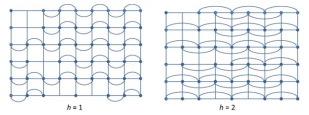
Geological Attribute Data Mining. When to study and research the relation among spatial points,
we can find that distance h changes, an attribute function of them changes accordingly. When distance h is changing to a certain value, the function can achieve good continuity and stability. It means a regularity rule is appearing. Different directions and different sampled points, the regularity rules are different. Every direction needs to find the best distance h can get the best continuity and stability. The distance h called “lag distance” in geostatistics.
The data mining process of geological attribute using lag distance h shows as Figure 1:
[image:3.612.152.461.473.588.2]
Figure 1. Data mining process of geological attribute using lag distance h.
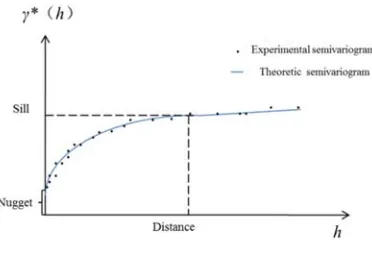
Figure 2. Experimental semivariogram fitting graphic.
Experimental Semivariogram Fitting. The number of samples is always limited in practice, so
[image:4.612.213.399.73.200.2]attribute difference points are discrete. People want to know continuous attributes and fit with a line through these discrete points, and this process called function fitting. People often use one line of known function to fit the discrete points and so such function called theoretic variogram. Semivariogram, which is an half of variogram, often used to describe regionalized variable. Also see Figure 2, which displays several important features (Burrough and McDonnell, 1998). The first is the “nugget”, a positive value ofγ(h) at h close to 0, which is the residual reflecting the variance of sampling errors and the spatial variance at shorter distance than the minimum sample spacing. The “Distance” is a value of distance at which the “sill” is reached, and provides information about the size of a search range in the spatial interpolation methods.
Search Anisotropy Ellipsoid and Its Parameters. According to curve line of semivariogram, we
can obtain corresponding Sill and Distance. The Distance is range of continuous and steady semivariogram line. In different directions, variation of regionalized variable is same but its continuity is different (same Sill, different Distance), which conditions called geometric anisotropy. The geometric anisotropy can transform into isotropy by simple geometric transformation, and there forms an isosurface (Sill) sphere with radius (Distance) changing in different directions in space. The process of simple geometric transformation is as following:
Set Distance d0 in one direction D0 as the base, and the relation between other direction Distances
and the base is: to Distance d1, K1=d1/d0; to Distance d2, K2=d2/d0; to Distance d3, K3=d3/d0. Bring
them into theory model and reflected in different components of a vector h.
o
d1 d2 d3
d0
D0 D1 D2
D3
Sill
γ(h)
0
y1 y2
d3 d0
h kh
γy1(h)
γy2(kh)
h Figure 3. Two dimension anisotropy transformation (a). Figure 4. Two dimension anisotropy transformation (b).
For the ratio is identical in same direction, the graphic shape obtained is an ellipsoid. So, we just consider difference of major axis and minor axis, which is the relation of Distance of d0’s direction
and d3’s. See also Figure 3 and Figure 4.
Let d0 as u direction and d3 as v direction, and both of major axis and minor axis are
mutually-perpendicular. So that vector h can be transformed into 2 2 3
' u ( v)
[image:4.612.118.494.507.614.2]
Figure 5. Two dimension anisotropy transformation (c). Figure 6. Three dimension anisotropy ellipsoid.
Similarly, isosurface in all directions can be obtained with the estimated point as the center coordinates, and so the geometric anisotropy isosurface in three dimensions (3D) space --- an isosurface sphere is achieved, as Figure 6 shows.
It is obtained by above process that Anisotropy ellipsoid and its parameters of geological attribute distribution in space. In specific operation, the first is to get regular shape orebody subdivided; and secondly, regionalized variable used as a data mining tool to get variogram line in all directions; and the last is to transform anisotropy by linear transformation and get parameters of major axis, semimajor axis and minor axis of the ellipsoid sphere.
Data Mining of Power Exponent
Relation of Power Exponent and Distance between Sampled Points. It is theoretically possible
for all sampled points impact value of estimated point attribute. According to the first law of geography, the more the distance between sampled point and estimated point, the impact is smaller, and the nearer the distance, the impact is greater. Weights diminish as the distance increases, especially when the value of the power exponent increases. The factor affecting the accuracy of IDW is the value of the power exponent (Isaaks and Srivastava, 1989). So the power exponent of DPIRM can be considered a function that depends on the distance, formula (5) as following:
PE (i) = f (D (i)) (5) Where PE (i) is power exponent depends on the distance D (i) between estimated point and sampled point i. According to different demands and practical applications, the function of power exponent has three situations:
1. The power exponent PE (i) is a constant, when the situation does not require high precision and not consider the relation of power exponent and the distance D (i). For example, when the power PE
is the constant 2, the most popular choice, and the resulting method is often called inverse square distance or inverse distance squared(IDS).
2. The power exponent PE (i) just depends on the length of distance D (i) .In this situation, only the change of D (i) distance length to be considered with variation of power exponent PE (i), and without direction of the distance D (i).
3. The power exponent PE (i) depends on the vector of distance D (i). In this situation, variation of power exponent not only considers the change of distance length but also the impact of different directions.
So corresponding relations of samples geological attribute and power exponent can be extracted with length or/and direction of distance.
Method of Finding the Best Power Exponent. If we calculate any sampled point value gi using
the observed value of other sampled points g1, g2, …, gn, the difference between estimated value and
observed value can be used to evaluate the calculating method and its parameters. This is called Cross Validation. According to the cross validation, a series of differences can be obtained with a series of different power exponents, as formula (6):
' 2 1 ( ) n i i i
S g g
(6)Where S is standard deviation of all sampled points observed values and estimated values, gi is the
observed value of sampled point i, gi’ is the estimated value using other points’ observed values.
From this formula, we found that the S is smaller, the calculating method and its parameters are better.
Search the Best Power Exponent by MATLAB GATBX. This paper uses the GATBX (Genetic
Algorithm Toolbox) of Sheffield University to search the best power of IDW in MATLAB 2013a.
1. Population Initialization Genetic Algorithm (GA) cannot calculate with the power
exponent of IDW directly before it is coded as chromosome.
(1) Coding Power exponent p is coded by binary coding, it ranges from 0 to 100 and 2 decimal
places can meet the requirement of precision. A formula (7) transferred the data to bit string in binary coding:
1 2
2m (100 0) 10- ≤2m- 1
(7) Where m is the length of bit string, and m =14 as the length of chromosome in GA.
(2) Decode Return the result from binary to decimal, the data transferred by the following formula (8):
max min
min ( )
2m 1
p p
pp Dec y
(8) Where pmin is the minimum value of power exponent p and pmax is the maximum value, y is the
corresponding binary value of p, Dec is the transformer from binary to decimal.
(3) Establish Initial Population The number of population is set to 40 (NIND = 40), the max
number of the evolutionary generations is set to 100 (MAXGEN = 100).
2. Individual Fitness Function Power exponent p is evaluated by cross validation and an
indicator, which is MSE (Mean Square Error) between observed values and calculated values of sample points.
The calculated values of sample points are from IDW with a different p at a time. The Individual Fitness Function formula (9) is as follows:
1 2
1
' 1 2
1 2 1
' 2
1
1 1 1 1
( ) ( ) ( ) ( )
1 1 1 1
( )
n n i
p p p p
i n i
j n
p p p p n i i n
j j j
C C C C
d d d d
C
d d d d
C C S n
(9) Where 'j
C is the calculated value of the point j, Cj is the observed value of the point j, di is the
distance between point i and point j, p is power exponent and S is MSE between observed value and calculated value.
3. Selection This case chooses some individuals to regroup a new population based on a
probability through a roulette wheel.
(1) The probability of individual fitness guarantees that individual with better fitness can survive into the next generation. If the number of a population is M, the fitness of individual Ui is fi, and the
1 i i M
k k
f P
f
(10) (2) Cumulative probability Qk of every individual can be calculated by the following formula (11):1 k
k j
j
Q P
(11)Where j=1, 2, …….
(3) r is a generated randomly between 0 and 1.
(4) If r ≤Q1, individual U1 is selected, if not, Uk will be selected ( 2≤ k < size of population),
so that makes the following formula (12) work.
1
k k
Q ≤ r ≤Q (12)
4. Crossover probability This case sets the crossover probability Px=0.7 as GATBX’s default.
5. Mutation probability This case sets the crossover probability Pm=0.017 as GATBX’s default.
An Illustrative Example and Validation
Procedure of IDPIRM Based on Spatial Data Mining Technique
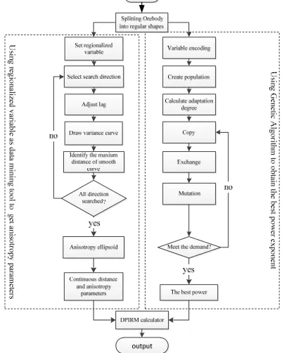
[image:7.612.205.407.367.618.2]The procedure of IDPIRM based on spatial data mining technique as Figure 7 shows:
Figure 7. Process flow chart of IDPIRM based on spatial data mining technique.
The steps of procedure of IDPIRM are the followings:
1. Try to Split unregular orebody into regular geometric parts, if possible. 2. Set some geological attribute as regionalized variable;
3. Use the regionalized variable as a data mining tool to achieve variogram curve in every direction, and identify the maximum smooth and continuous distance;
4. Search in all directions? Yes, go to the next step, or go to step 3.
6. Encoding variable for Genetic Algorithm program. 7. Create initial population;
8. Calculate adaptation degree to select the better individuals. 9. Copy the better individuals’ gene.
10. Exchange genes among the population. 11. Mutate genes among individuals.
12. Calculate adaptation degree. Does adaptation degree meet preinstall demand? Yes, go to next step, or go to step 9, until the adaptation degree meet the preinstall value or the number of generations reach the preinstall number.
13. Decode the best individual, and get the best power exponent.
14. Bring parameters of the anisotropy ellipsoid and the best power exponent into DPIRM calculator to interpolation.
15. Output the result of interpolation, and end it.
Practical Example of One Copper Open-pit and Test
A copper open-pit is one of large-scale and low-grade non-ferrous mines, which has the features of huge ore reserve, low grade and polymetallic. The metallogenic belt looks like a long ring, the major axis is 2600m, and the minor axis is 1350m. The direction of strike about 50°, northwest dip, gradually turns 85º to 75º from east to west. Both of two turning points at north and south inclined inward, 60ºinclination. The width of a barren core body is 900m in the middle of north ringlike belt; the width of a barren core body is 150~850m in the middle of south ringlike belt. Ore bodies have phenomenons as dilatation, striction, offset and recombination along the direction of strike and tilt. The cover of upper orebody is thin, average thickness 25m, and many places are outcropping along the strike. The main faults, f7and f8, split orebody into two parts of the south and the north.
Due to the orebody shape is complex, it is unreasonable and imprecise that only one anisotropy ellipsoid’s parameters are used to estimate Cu grade and reserve of this orebody. According to the geology of this orebody, the main faults f7, f8 and an exploration line are used to split the Cu orebody into five parts: the south orebody, the middle orebody, the north 01 orebody, the north 02 orebody and the north 03 orebody, show as Figure 8:
Figure 8. Five parts of a copper ore-bed. Figure 9. Relation of power & samples cross validation’s standard deviation.
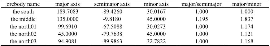
[image:8.612.88.524.653.728.2]With a mining software, such as Surpac, a geological database was Created and five statistical analysises of the orebodies were made individually; And Cu grade was set as the regionalized variable and variagrom lines were drawed. According to the smooth continuity of these variogram lines, the parameters of spatial anisotropy ellipsoids IDPIRM need were achieved (see Table1).
Table 1.Anisotropy ellipsoid parameters of five orebodies.
orebody name major axis semimajor axis minor axis major/semimajor major/minor
the south 189.7083 -89.4260 30.0167 1.000 1.000
the middle 135.0000 -9.8180 45.0000 1.195 1.837
the north01 99.6910 -67.5088 30.0273 1.000 1.174
the north02 45.0000 -79.7638 45.0000 1.000 1.121
the north03 94.9081 -89.9863 32.7822 1.000 1.168
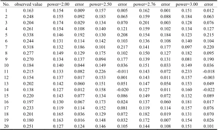
From this picture, we can see that the power exponent and the standard deviation of sampled points Cu grade together drawed a parabola going upwards. It is the best power exponent that the lowest of the parabola, the power is 2.76 and its cross-validation standard deviation is 1.1785. Some sampled points’ estimated values and observed values based on different power exponents as Table 2.
Table 2. Some sampled points’ estimated value and observed value based on different power exponents.
No. observed value power=2.00 error power=2.50 error power=2.76 error power=3.00 error
1 0.163 0.154 0.009 0.157 0.005 0.162 0.001 0.151 0.012
2 0.248 0.155 0.092 0.183 0.065 0.159 0.088 0.184 0.063
3 0.204 0.174 0.029 0.134 0.070 0.201 0.003 0.128 0.076
4 0.261 0.154 0.108 0.140 0.121 0.159 0.102 0.134 0.127
5 0.338 0.146 0.192 0.130 0.208 0.154 0.184 0.123 0.215
6 0.244 0.131 0.114 0.142 0.103 0.136 0.108 0.140 0.104
7 0.318 0.132 0.186 0.101 0.217 0.141 0.177 0.097 0.220
8 0.277 0.149 0.129 0.175 0.102 0.150 0.127 0.182 0.095
9 0.270 0.134 0.137 0.094 0.177 0.139 0.131 0.081 0.190
10 0.184 0.140 0.044 0.149 0.036 0.151 0.033 0.149 0.036
11 0.215 0.133 0.082 0.226 -0.011 0.143 0.072 0.233 -0.018
12 0.154 0.137 0.017 0.153 0.001 0.143 0.011 0.157 -0.003
13 0.202 0.142 0.060 0.151 0.051 0.147 0.054 0.153 0.049
14 0.138 0.127 0.012 0.158 -0.020 0.127 0.011 0.160 -0.022
15 0.220 0.143 0.077 0.134 0.086 0.149 0.072 0.132 0.089
16 0.197 0.130 0.067 0.173 0.024 0.137 0.060 0.181 0.017
17 0.233 0.119 0.114 0.152 0.081 0.119 0.114 0.157 0.076
18 0.201 0.165 0.036 0.129 0.072 0.182 0.019 0.131 0.070
19 0.180 0.163 0.016 0.148 0.032 0.172 0.007 0.154 0.026
20 0.251 0.127 0.124 0.146 0.105 0.144 0.108 0.151 0.101
Input the parameters of anisotropy ellipsoid and the best power into DPIRM to obtain the spatial interpolation of this Cu open-pit. Besides this new interpolation, we have interpolated for this Cu orebody with Ordinary Kriging, traditional Inverse Distance Square (IDS), the south part of results comparison table See Table3. Other four parts are similar, which confined to the length of this paper and not to present.
Table 3. Three interpolation methods’ Cu grade results comparison table (the south).
the south IDPIRM (power=2.76) Ordinary Kriging Traditional IDS
grade interval
region(%) grade(%) average metal (t) grade(%) average metal (t) grade(%) average metal (t)
0.0 -> 0.1 0.09 242.22 0.09 246.82 0.09 238.26
0.1 -> 0.2 0.15 5722.07 0.15 5676.41 0.15 5535.46
0.2 -> 0.3 0.23 3341.55 0.24 3456.60 0.24 3431.80
0.3 -> 0.4 0.33 708.67 0.33 663.23 0.33 810.15
0.4 -> 0.5 0.42 3.75 0.41 3.23 0.44 219.93
0.5 -> 0.6 0.00 0.00 0.00 0.00 0.53 49.92
0.6 -> 0.7 0.00 0.00 0.00 0.00 0.63 8.00
0.7 -> 0.8 0.00 0.00 0.00 0.00 0.76 2.06
0.8 -> 0.9 0.00 0.00 0.00 0.00 0.84 1.31
0.9 -> 1.0 0.00 0.00 0.00 0.00 0.00 0.00
sum 0.17 10018.27 0.17 10046.30 0.18 10296.93
Conclusions
[image:9.612.89.524.499.685.2]mining technology, the results of interpolation can be precision and reliability. Avoiding the isotropy problem of traditional DPIRM, New Distance Power Inverse Ratio Method (IDPIRM) uses regionalization variable theory to get the law of spatial data distribution, and uses artificial intelligence algorithms as another data mining technique, just like Genetic Algorithm, to find the best power exponent of DPIRM without subjective effect of operator. If so, the precision and the reliability of interpolation result are improved.
Conclusions:
(1) Geological spatial interpolation should be based on spatial data mining;
(2) Regionalized variable theory as One of Spatial data mining can amend the isotropy fault of traditional DPIRM.
(3) The spatial data mining based on the Cross Validation with Genetic Algorithm Toolbox of MATLAB, can achieve the best power exponent with its objection and reliability.
(4) It is spatial data mining technique, as Semivariogram and GA, that can do contribute to the accuracy of DPIRM.
Acknowledgements
This research was partially supported by 2017 Intelligent Manufacturing Comprehensive Standardization Project (Grant No. Z135060009002), the National Natural Science Foundation of China (Grant No. 51104010) and the Fundamental Research Funds for the Central Universities (Grant No. FRF-SD-12-001A). Additional support has been provided by State Key Laboratory of High-Efficient Mining and Safety of Metal Mines (University of Science and Technology Beijing), Ministry of Education.
References
[1] Zhang Lihua, Jia Shuaidong, Wu Chao, et, al. A Method for Interpolating Digital Depth Model Considering Uncertainty. J. Acta Geodaetica et Cartographica Sinica, 2011(3): 359-365.
[2] Wang Zhimin, Application of Fractal Theory to the Estimation of Ore Body’s Grade by the Reverse K Square Distance Method. J. China’s Manganese Industry, 1997(2): 19-22.
[3] Li Z., Li X., Li C., et al. Improvement on inverse distance weighted interpolation for ore reserve estimation [C]. 2010, p. 1703-1706.
[4] Jiang Quan, Chen Jianhong, Wang Liguan, et, al. Dynamic Reserve Calculation of a Low Alumina-Silica Ratio Thin Orebody via Visual Simulation. J. Science & Technology Review, 2010(19): 36-41.
[5] Luo Zhouquan, Zhang Bao, Liu Xiaoming, et, al. 3D Visualization Method of Analysis and Estimation of Orebody Grade and Reserves. J. Nonferrous Metals(Mining Section), 2008(5): 23-27.) [6] Li Zhang-lin, Zhang Xia-lin. Designing and Realization of Mineral Resources Reserve Calculation Module Using Inverse Distance Square Method. J. Geology and Prospecting. 2007(6): 92-97.
[7] Li Zhanglin, Wang Ping, Li Dongmei. Application and research of a new interpolation calculated method. J. China Mine Engineering, 2008(1): 39-43.
[8] Zhuang Liwei Wang Shili. Spatial Interpolation Methods of Daily Weather Data in Northeast China. J. Quarterly Journal of Applied Meteorology, 2003(5): 605-615.
[10] Wang Tie; Jin Zhiqiu; Wang Zhihong. Improvement and Parameter Optimization of Distance Power Inverse Ratio Method. J. China Mining Magazine. 1994(4): 47-50.
[11] Lao Jinghua, Yu Dongming. Spatial Data Interpolation Methods in Orebody 3D Simulation Technology. J. Popular Science & Technology. 2008(8): 100-101.
[12] Pan Guocheng, Li Xiufeng. Several practical problems of reserve estimation in Geostatistics application(1). J. Foreign Metal Mining Magazine, 1996, 21(7): 7-12.
[13] Pan Guocheng, Li Xiufeng. Several practical problems of reserve estimation in Geostatistics application(2). J. Foreign Metal Mining Magazine, 1996, 21(008): 5-9.
[14] Li Cui-ping, Zheng Yao-xia, Zhang Jia, et, al. Ore grade interpolation model based on support vetor machines optimized by genetic algorithms. J. Journal of University of Science and Technology Beijing, 2013(7): 837-843.
[15] Huang Guangqiu, Gui Zhongyue. A Genetic Algorithm Approach to Determining Optimum Parameters of Distance Power Inverse Ratio Method [J]. China's Manganese Industry, 1997,1 5(3)20-25.