2017 International Conference on Mathematics, Modelling and Simulation Technologies and Applications (MMSTA 2017) ISBN: 978-1-60595-530-8
Parallel Implementation of the Coordinates-partitioning Based
Aggregation-type Algebraic Multigrid Preconditioners
Jian-ping WU
*, Jun ZHAO and Shu-chang WANG
College of Meteorology and Oceanography, National University of Defense Technology, Changsha, China
*Corresponding author
Keywords: Aggregation based algebraic multigrid, Sparse linear system, Coordinates partitioning, Preconditioner, Conjugate gradient method, Parallel algorithm.
Abstract. The coordinates-partitioning based aggregation-type algebraic multigrid preconditioners have been proven to be very efficient in the solution of sparse linear systems with conjugate gradient iterations. In this paper, a parallel algorithm for the setup is provided and the parallelization of the preconditioning process is also considered. The parallel algorithm is based on a good property of the coordinates-partitioning based aggregation, that is, the aggregation process is performed in a fashion from the coarsest level to the finest step by step. Thus, the original adjacent graph is partitioned into a number of sub-graphs, where each sub-graph is related to a node in the coarsest level and is assigned to a processor. The aggregation process can then proceed forward on each processor independently from the assigned sub-graph. When this kind of multigrid preconditioner is applied in Krylov subspace iterations, only the computation on the coarsest level and the matrix-vector multiplications related to the smoothing on each level require communication for V- and W-cycle versions, and require only some extra communication related to dot products for the K-cycle version. The size of the derived linear system on the coarsest level can be controlled by the adjustable arguments and this system can be solved again in parallel with some preconditioned Krylov subspace iterations. The structure information related to the matrix-vector multiplications is invariable to the iterations and can be derived in the setup and be stored, and is used in the latter iterations. Finally, the parallel algorithm is validated for the Gauss-Seidel smoother and some kinds of popular multigrid cycles in solving sparse linear systems from some two-dimensional model partial equations with preconditioned conjugate gradient iterations. The results show that the parallel efficiencies of both the setup and the iteration processes are satisfied.
Introduction
The solution of sparse linear systems occupies much part of the whole run time in many scientific and engineering applications, and many methods have been presented to solve this kind of system. Among them, the Krylov subspace iteration [1] and the multigrid method [2] are the two most famous. Especially, multigrid methods can be incorporated with Krylov subspace iterations to exploit both the potential of optimal convergence rate of the former and the robustness of the latter, where the multigrid method is used as the preconditioner.
There are several types of algebraic multigrid methods, among which the classical-type and the aggregation-type are two most frequently used ones. The classical type converges more rapidly in general, but is more expensive. In addition, the setup process is hardly to be parallelized. The aggregation type is simpler and cheaper for the construction process. Up to now, there are two ways to determine the interpolation operators, the classical method [3] and the method based on smoothing[4]. The former is very simple and cheaper. The latter can lead to more rapid convergence at the cost of more non-zero entries and more complex non-zero structures. Whichever way is used, it is required to construct the grid hierarchy first.
The most famous aggregation scheme is based on the concept of strong connection, where two end-points of the edge with maximum weight are aggregated into a coarse point [5]. It can be repeatedly applied to reduce the number of levels. The frequently used scheme is to repeat the process two or three times [6], that is, there are four or eight points put into an agglomeration at most respectively. To maintain the element structure, a coarsening scheme is provided based on concentrating three points each time [7]. To improve the quality of the grid hierarchy, each point not assigned to any aggregation can be added to an adjacent one as soon as possible [4]. Braess provided a scheme based on grouping each two points with maximum edge weights into one subset first, and then aggregating each two subsets with the maximum number of edges into an aggregation [8].
Wu et. al. provided a two-level grid correction for parallel incomplete factorization based on partitioning of the adjacent graph, with each part corresponding to a coarse grid point [9]. Kumar also provided a two-grid algorithm based on graph partitioning, with each sub-graph corresponding to an aggregation, where ILU(0) and ILUT are selected as the smoother and the solution scheme for the coarsest problem [10]. In reference [11], several frequently used aggregation schemes are tested and the experiments show that the best is always among the two-point scheme and its variants.
While the application process of algebraic multigrids is relatively ready to be parallelized, the parallelization of the setup process is much more difficult. In classical algebraic multigrids, it can be mainly reduced to the parallel section of the coarser grid points [12]. In aggregation based versions, the focus is the parallel section of the aggregations. Adams provided an aggregation scheme based on the maximal independent set algorithm [13]. Tuminaro et al provided three parallel schemes [14], a scheme coarsening in each processor independently. In [15], several parallel aggregation strategies are compared, and the results suggest that the types aggregating from the borders to the interiors are the best. In [16], parallelization techniques for multigrid solvers are surveyed, and parallel coarsening is one of the focuses.
In aggregation based algebraic multigrids, the aggregation process is in general based on local connectivity. Though for parallel computing, the original adjacent graph can be partitioned into sub-graphs and then apply aggregating schemes to them individually. The graph based aggregation has been used for two-level grid methods in [9] and [10], and in [17], such kind of method is provided for algebraic multigrid methods, where the construction starts from the coarsest grid to the finest one step by step. Each coarse-grid point is an aggregation of several fine-grid points and the number can be selected as needed. The test results have validated its effectiveness. In this paper, the parallelization for this scheme will be considered.
The Coordinates-Partitioning Based Aggregation-Type Algebraic Multigrid Preconditioner
Consider the following sparse linear system
Au=b, (1)
where A is a known n by n sparse matrix and is symmetric positive definite, b is a known vector of
length n, and u is the unknown vector. The linear system (1) can be solved with preconditioned
conjugate gradient (PCG) iterations [1], where the preconditioner is selected as the aggregation based algebraic multigrid in this paper.
approximation solution can be given by u(l) = Ll-1b(l) on level l, where Ll is a smoother. The related
residual vector r(l) = b(l) - Al x(l) is restricted to level l+1, multiplying (Pl+1,l)T from the left. For matrix
Bl=(Pl,l+1)TAl is invariant in the PCG iterations, it can be pre-computed in the setup process. On level
l+1, the algorithm is invoked again to derive the correction vector v(l+1). It is interpolated back to level l, to correct the approximation u(l). And then a post smoothing is applied to u(l) with the smoother LlT.
In this algorithm, we can select Gauss-Seidel iteration as the smoother. In this case, Ll is a matrix
with Ll(i,j)=Al(i,j) for j=1 to i and i=1 to nl, and all others zero. Besides (Pl,l+1)TAl, the grid hierarchy,
Al, Pl,l+1, and Ll are also unchanged during the PCG iteration. Therefore, they can also be
pre-computed and put into the set-up process beforehand, and be used directly in latter PCG iterations. In addition, the grid hierarchy is the kernel of this process, which is determined by the aggregation scheme. Once the grid hierarchy is determined, the other parts can be determined from it directly. Specially, when the simple classical interpolation operators are used, the coefficient matrix on a coarser level can be derived by first summation of the corresponding rows and then of the corresponding columns of the matrix on the finer level.
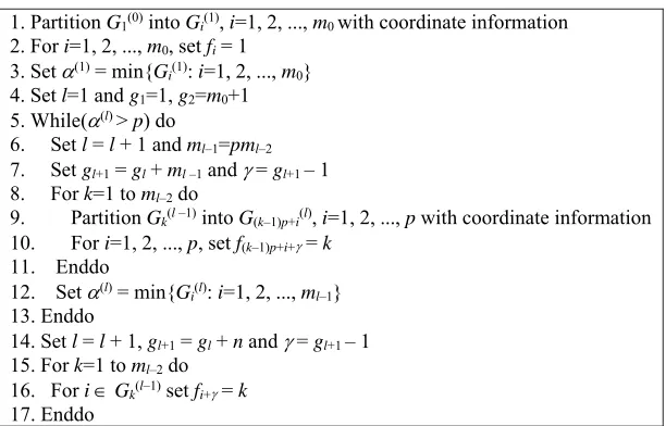
Assume that linear system (1) is derived from a certain partial differential equation and the coordinate information related to each unknown is given. Then the aggregation algorithm based on coordinates partitioning [17] can be described in detial as figure 1, where the input arguments are the coordinates of each unknown, m0, p and G1(0), the adjacent graph of the coefficient matrix A. For A is
symmetric, G1(0) is undirected. The output is l, array f and g. The graph G1(0) is partitioned into m0
parts firstly and then each part is recursively partitioned into p parts, until the minimal size of some
sub-graph on some level is not larger than p.
On output, a grid hierarchy is derived and the number of levels is given by the output argument l.
For k < l, each sub-graph Gi(k) is corresponding to a point in level k. And for level l, each point is
corresponding to a point of G1(0). The value fi records the label of the corresponding node in the
coarser level of i, and gk is the position of the first value of level k in vector f. Therefore, the 1st level
has m0 nodes, the 2nd level has pm0 nodes, the 3rd level as p2m0 nodes, and so on. The (l–1)-th level
has pl–1m0 nodes and the l-th level has n nodes.
Now we can reverse the grid hierarchy to setup the multigrid. The k-th level in the multigrid can be
regarded as the (l+1–k)-th level in figure 1. Then in the multigrid, the 1-st level has n nodes and the
coarsest level is the l-th one, which has m0 nodes. The nodes and the corresponding coefficient matrix
in the 1st level have known beforehand, that is ml=n and A respectively. For level k > 1, the nodes is
given by fi+ for each node in level k–1, that is, for i=1, 2, ..., ml–k, where = gl+1–k –1. The nodes with
the same fi+ are aggregated into a node in the coarser level k.
1. Partition G1(0) into Gi(1), i=1, 2, ..., m0 with coordinate information
2. For i=1, 2, ..., m0, set fi = 1
3. Set (1) = min{G
i(1): i=1, 2, ..., m0}
4. Set l=1 and g1=1, g2=m0+1
5. While((l) > p) do
6. Set l = l + 1 and ml–1=pml–2
7. Set gl+1 = gl + ml –1 and = gl+1 – 1
8. For k=1 to ml–2 do
9. Partition Gk(l –1) into G(k–1)p+i(l), i=1, 2, ..., p with coordinate information
10. For i=1, 2, ..., p, set f(k–1)p+i+ = k
11. Enddo
12. Set (l) = min{G
i(l): i=1, 2, ..., ml–1}
13. Enddo
14. Set l = l + 1, gl+1 = gl + n and = gl+1 – 1
15. For k=1 to ml–2 do
16. For iGk(l–1)set fi+ = k
[image:3.612.154.460.504.700.2]17. Enddo
Combining all the issues above, the whole setup process can be described as figure 2, where ibJk
and jJk are used to store the aggregations in CSR format. In figure 2, step 8 is used to compute a ILU(0)
factorization, which is used as the preconditioner of the sparse linear system on level l. In this paper,
this system will be solved with preconditioned conjugate gradient iterations again.
1. Invoke algorithm ACRP with m0, p and matrix A, deriving l, f and g
2. For k=1 to l–1 do compute mk = gk+2 – gk+1
3. For k=1 to l–1 do
4. Compute ibJk, and jJk with ml–k, ml–k+1 and f(gl–k+1: gl–k+1+ml–k)
5. Compute Bk = (Pk,k+1)TAk
6. Compute Ak+1= BkPk,k+1
7. Endfor
[image:4.612.164.448.126.219.2]8. Compute ILU(0) factorization of Al
Figure 2. The setup process based on algorithm ACRP described as figure 1.
Parallel Implementation of the Coordinates-Partitioning Based Multigrid Preconditioner
Though there are several ways to parallelize a given algorithm, only the message passing version is considered here. The message passing interface (MPI) is used and the parallel algorithms are based on the domain decomposition method. Assume that the linear system (1) has been distributed to P
processors, with approximately even number of rows of the coefficient matrix A assigned to each
processor. For simplicity, we assume that the rows assigned to each processor have contiguous indexes. The components of all the vectors on each level are assigned to the processors according to the rows of the coefficient matrix. In the parallelization of PCG iteration and the multigrid algorithm, the results of the inner products are repeatedly stored on all processors. Therefore, the inner products are done with the MPI function MPI_Allreduce. In this way, to complete the whole parallel implementation, the remaining components includes the partitioning algorithm ACRP, the setup process described as figure 2, the smoothing steps in the application of multigrid, the multiplication of matrices to a vector.
To paralleling the algorithm ACRP, it can be done by replacing G1(0) in figure 1 with the local part.
It should be noted that we only know the rows of A assigned to this processor, which can be regarded
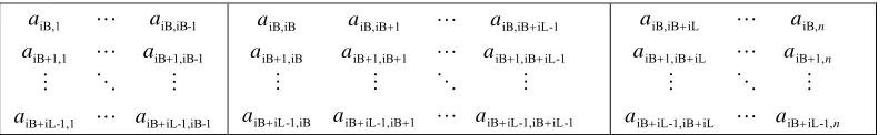
as a sub-matrix. It can be illustrated as figure 3. Without loss of generality, we assume that rows assigned to this processor have indexes from iB to iB+iL–1, where iB is the index of the first row and iL is the number of rows. But the column indexes may ranging from 1 to n. To derive the local version
of G1(0), we can preserve the entries with column indexes ranging from iB to iB+iL–1, and then
subtracting iB–1 from each index. Then we can apply the algorithm ACRP with the derived local version on all processors in parallel. The only operation requiring communication is the computation of (l), that is, step 3 and 12 in figure 1, such that the number of levels l is the same for all processors.
In addition, for the first several levels, communications may not be needed at all. Only if the number of nodes in each sub-graph is small enough, the communication step is required. In this paper, for simplicity, this saving in communication is not considered. The MPI function MPI_Allreduce is used for each level instead.
1 -1,iB -iL iB 1,1 -iL iB 1 -1,iB iB 1,1 iB 1 -iB,iB iB,1 a a a a a a 1 -iL iB 1, -iL iB 1 iB 1, -iL iB iB 1, -iL iB 1 -iL iB 1, iB 1 iB 1, iB iB 1, iB 1 -iL iB iB, 1 iB iB, iB iB, a a a a a a a a a n n n a a a a a a 1, -iL iB iL iB 1, -iL iB 1, iB iL iB 1, iB iB, iL iB iB,
Figure 3. Schematic diagram of matrix elements assigned to a processor.
[image:4.612.109.509.607.668.2]the convergence rate can be expected to very fast even if much cheaper preconditioner is used. Thus, in parallel computation, a block diagonal analog can be used as the preconditioner, where Al is firstly
approximated by a diagonal block matrix, with one block on each processor, and then ILU(0) is performed to each block locally. Step 5 means to perform a summation over all the rows related to each aggregation. The row on the coarser level related to an aggregation is on the same processor as those related to its entries. Therefore, there are no communications. Step 6 means to perform a summation over the columns, which requires no communication too. But the column indexes are global, ranging from 1 to ml–1 for level l, therefore, a column derived from the summation over the
columns related to the same aggregation will have a global column index too, which is given by the corresponding component of the vector f. Before summation, we should know that which aggregation
is in for each column. Thus a global snapshot of the aggregations over all the processors should be derived on each processor.
To get the global snapshot of all the aggregations, three steps are required. First, we should derive the number of points on all processors in each level. If denote the number of points on processor i as ni,k for level k in multigrid, then we know that for level 1, ni,1 is different from each other, so they
should be passed to all the processors, which can be implemented with the MPI function MPI_Allgather. For level k>1, the number of local points must be m0pl-k on every processor.
Therefore no communication is required. Second, the number of points in each aggregation should be known on each processor. By the construction, for the first level, it is variable for different aggregations. But for level k>1, it is equal to p all the time. Thus, communication is required for the
first level only and it can be implemented with MPI_Allgatherv. Finally, the indexes of the points in all the aggregations should be known. For the same reason as for the number of points in each aggregation, communication is required for the first level only again and it can also be done with another MPI_Allgatherv. For level k>1, each processor has m0pl-k points, and each aggregation has p
points, thus for each point on this level, the aggregation index can be computed directly.
For the multiplication v=Au, if there a matrix entry with column index j not in iB to IB+iL-1, where
iB and iL are the same as before, the j-th component of u must be on other processors and should be
received from the related processor. As for v, the components can be classified into two classes. Some
components of v will not depend on any components of u belonging to other processors, which is
called the interior components. The others are called the border components. Therefore, the computation of the interior component can be done in parallel on all the processors. At the same time, for the components of u which the border components depend on, a non-blocked receive operation
can be issued. And the corresponding send operations can be issued too. After the computation of the interior components, the MPI_Wait function can be used to wait the receive operations to complete. Once they are completed, the computation of the border components is followed. In this way, the computation and the communication can be overlapped. The multiplication of Al to a vector u(l) and
the multiplication of Bl to a vector u(l) is very similar. The only difference is that Bl has less rows than Al. It should be noted that the structure information used in the multiplication will be invariable to the
PCG iterations, including the number of components received from each processor, the number of components sent to each processor, the component indexes received and sent, and so on. This invariable information can be computed in the setup process and be used in the iterations directly.
For the smoothing process in the application of multigrid, we can approximate Ll with a diagonal
block matrix in a similar way to the parallelization of ILU(0). Then each processor can compute a local part of u(l) independently. Correspondingly, the post smoothing should be used on the condition
that Ll is replaced by this block version, to ensure the symmetric property of the preconditioner,
which is vital to the convergence of the PCG iterations. Apparently, the computation in the brackets can be done in a similar way to the operation Alu(l). And the multiplication of Ll–T to the result can be
Numerical Experiments
In this section, all the experiments are performed on a cluster of workstation, which has 32 nodes, with two processors on each node. The processor is Intel(R) Xeon(R) CPU E5-4640 0 @ 2.40GHz (cache 20480 KB). The operating system is Linux version 2.6.32-431.el6.x86_64 and the compiler is Intel FORTRAN Version 15.0.0.090. The MPICH version 3.1.3 is used for communication between processors. For the initial linear systems, they are distributed to processors according to the way mentioned in section 3 and the partitioning scheme is the same as step 1 and 9 in figure 1. After partitioning, the rows assigned to a processor may have discontinuous indexes. Therefore, they are relabeled such that the indexes are continuous on every processor and the indexes on processor k are
all less than those on processor k+1 for k=0 to P-2. The column indexes are relabeled correspondingly.
When solving a linear system with multigrid preconditioned conjugate gradient method, for the outer PCG iteration, the initial approximation is selected as zero all the time and the stop criterion is selected as the 2-norm of the residual vector is reduced by 1E-10. For the inner PCG iteration on the coarsest level, the linear system is solved with preconditioned conjugate gradient too, and the initial approximation is selected similarly, while the stop criterion is selected as the 2-norm of the residual vector is reduced by 1/10. During the coarsening process, the number of nodes on the coarsest level for each processor is selected as m0=1024/P, where P is the number of processors. This selection can
ensure that the order of the linear system on the coarsest level is m0, invariable to the number of
processors. Thus, the number of levels are almost the same too for different number of processors. Two numerical experiments are done for discrete linear systems derived from a model partial differential equation with finite difference schemes, denoted as Lin1 and Lin2 respectively. They are derived from the following PDE problem with Dirichlet boundaries
– 2u/x2 – 2u/y2 = f, (2)
where x, y (0,1) and the function f and the boundary values are given from a true solution u=1. In
the discretization, n+2 discrete points are selected in each dimension and u(xi, yj) is denoted as ui,j for
any function u, where
xi = ih, yj = jh, i, j = 0,1, …, n+1,
and h=1/(n+1). For Lin1, The discrete form is
– ui,j–1 – ui–1,j + 4ui,j– ui+1,j– ui,j+1=h2fi,j. (3)
For Lin2, the following discrete form is used
– ui–1,j–1 – ui,j–1– ui+1,j–1 – ui–1,j + 8ui,j– ui+1,j– ui–1,j+1 – ui,j+1– ui+1,j+1=h2fi,j. (4)
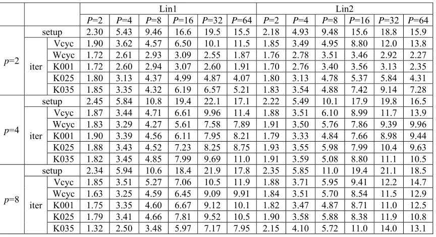
In the experiments, n is selected as 2048 for both linear systems. The results are given in table 1. In
the table, Vcyc and Wcyc mean the V- and W- cycle multigrid respectively, and K001, K025, K035 denote the K- cycle multigrid with t=0.01, t=0.25, and t=0.35 respectively. The sign setup and iter
mean the setup and the iteration process respectively. The speedup is derived from the time on one processor to the parallel execution time for the same cycle.
From table 1, it is clear that for the linear system Lin1, when the number of points aggregated each time is 2, the speedup for the setup is increased step by step until 32 processors used for each cycle. When 64 processors is used, the speedup is worse than that for 32 processors. The speedup is increased step by step for V-cycle until 64 processors. For K-cycle with t=0.35, the maximal speedup is reached when 32 processors is used. For other cycles, the maximal speedup is reached when 16 processors is used instead. When 32 processors is used, approximately 20x speedup can be achieved for the setup process. As for iteration, the maximum speedup is achieved for V-cycle when 64 processors used, which is approximately 11.5.
achieve approximately 22x speedup and the iteration process can achieve 11.4x speedup for V-cycle, which is maximal over all the cycles. When 8 points are aggregated each time, the setup process can achieve the maximal speedup with 32 processors again, and the maximum is 21.9. The iteration process can achieve 11.9x speedup for V-cycle again, which is the maximum over all cycles.
Table 1. Speedup for the setup and iteration process when solving Lin1 and Lin2 using different schemes, where P is the different number of processors and p is the different number of points aggregated each time.
Lin1 Lin2
P=2 P=4 P=8 P=16 P=32 P=64 P=2 P=4 P=8 P=16 P=32 P=64
p=2
setup 2.30 5.43 9.46 16.6 19.5 15.5 2.18 4.93 9.48 15.6 18.8 15.9
iter
Vcyc 1.90 3.62 4.57 6.50 10.1 11.5 1.85 3.49 4.95 8.80 12.0 13.8 Wcyc 1.72 2.61 2.93 3.09 2.55 1.87 1.76 2.78 3.51 3.46 2.92 2.27 K001 1.72 2.60 2.94 3.07 2.60 1.91 1.70 2.76 3.40 3.56 3.13 2.35 K025 1.80 3.13 4.37 4.99 4.87 4.07 1.80 3.13 4.78 5.37 5.84 4.31 K035 1.85 3.35 4.32 6.19 6.57 5.21 1.83 3.54 4.88 7.42 9.14 7.28
p=4
setup 2.45 5.84 10.8 19.4 22.1 17.1 2.22 5.49 10.1 17.9 19.8 16.5
iter
Vcyc 1.87 3.44 4.71 6.61 9.96 11.4 1.88 3.51 6.10 8.99 11.7 13.9 Wcyc 1.83 3.29 4.27 5.61 7.58 7.89 1.91 3.50 5.76 7.86 9.39 9.96 K001 1.90 3.39 4.56 6.11 7.95 8.21 1.79 3.33 4.84 7.66 8.98 9.44 K025 1.88 3.43 4.52 7.23 8.25 8.75 1.93 3.55 5.98 7.99 10.4 9.63 K035 1.82 3.45 4.85 7.99 9.69 11.0 1.91 3.59 5.08 8.80 11.1 10.5
p=8
setup 2.34 5.94 10.6 18.4 21.9 17.8 2.35 5.85 11.0 19.4 21.1 18.5
iter
Vcyc 1.85 3.51 5.27 7.06 10.5 11.9 1.88 3.71 5.95 9.41 12.2 14.7 Wcyc 1.63 3.25 4.59 6.45 9.09 9.91 1.84 3.51 5.70 8.54 11.5 12.9 K001 1.75 3.35 4.60 6.67 9.12 10.1 1.82 3.47 4.87 8.71 11.0 12.5 K025 1.79 3.41 4.66 7.81 9.52 10.5 1.90 3.58 5.88 8.38 11.9 10.8 K035 1.32 2.50 3.48 5.97 7.17 7.95 2.15 4.10 5.72 11.0 14.0 13.1
For linear system Lin1, there are only 5 non-zero entries in each row of the coefficient matrix. Let us to investigate the cases when Lin2 is solved. For these cases, there are 9 non-zero elements in each row. From table 1, we can see that, for the setup, the speedup is always attained when 32 processors are used. For p=2, 4 and 8, the speedup attains 18.8, 19.8 and 21.1. As for the iteration time, the
speedup is always higher when the V-cycle is used. The maximum is approximately 14.
From the above analyses, it can be concluded that the parallel implementation provided in this paper is satisfied. The setup process can efficiently scale to 32 processors and the iteration process can scale to 64 processors for most of the cases, especially for the V-cycle multigrid preconditioner. For the cases with more non-zeros in each row of the coefficient matrix such as Lin2, the speedup is significantly higher. The maximal speedup for Lin2 can attain 14 or more, while for Lin1, it is about 12. In addition, it should be noted that, as for the iteration time, the K-cycle with proper parameter t will be better than the other cycles.
Summary
equations with preconditioned conjugate gradient iterations. The results show that the parallel efficiencies of both the setup and the iteration processes are satisfied.
Acknowledgement
This research was financially supported by the National Science Foundation of China(61379022).
References
[1] Y. Saad, Iterative methods for sparse linear systems, PWS Publication Corporation, Boston, 1996.
[2] R. Wienands, W. Joppich, Practical Fourier analysis for multigrid methods, Taylor and Francis Inc., 2004.
[3] C. Wagner, Introduction to algebraic multigrid, Course Notes, University of Heidelberg, 1998/1999; available at: http://www.iwr.uni-heidelberg.de/~Christian.Wagner/, 1999.
[4] Vanek P., Mandel J., and Brezina M., Algebraic multigrid by smoothed aggregation for second order and fourth order elliptic problems, Computing, 56(1996)179-196.
[5] H. Kim, J. Xu, and L. Zikatanov, A multigrid method based on graph matching for convection-diffusion equations, Numer. Linear Algebra Appl., 10(2003) 181-195.
[6] Notay, Y., An aggregation-based algrbraic multigrid method, Electronic Transactions On Numerical Analysis, 37(2010)123-146.
[7] Dendy, J.E., Jr., & Moulton, J.D., Black Box Multigrid with coarsening by a factor of three, Numerical Linear Algebra With Applications, 17: 2-3(2010)577-598.
[8] D. Braess, Towards algebraic multigrid for elliptic problems of second order, Computing, 55(1995)379-393.
[9] J.P. Wu, J.Q. Song, W.M. Zhang and H.F. Ma, Coarse grid correction to domain decomposition based preconditioners for meso-scale simulation of concrete, Applied Mechanics and Materials, 204-208(2012)4683-4687.
[10] P. Kumar, Aggregation based on graph matching and inexact coarse grid solve for algebraic two grid, International Journal of Computer Mathematics, 91: 5(2014)1061-1081.
[11] Wu Jian-ping, Yin Fu-kang, Peng Jun, Yang Jin-hui, Research on Aggregations for Algebraic Multigrid Preconditioning Methods, In: 2017 2nd International Conference on Computer Science and Technology [CST2017], Guilin, China, 2017.
[12] Henson, V.E., & Yang, U.M., Boomer AMG: A parallel algebraic multigrid solver and preconditioner, Applied Numerical Mathematics, 41: 1(2002)155-177.
[13] M.F. Adams, A parallel maximal independent set algorithm, In Proceedings 5th Copper mountain conference on iterative methods, 1998.
[16] E Chow, R.D. Falgout, J.J. Hu, R.S. Tuminaro, U.M. Yang, A survery of parallelization techniques for multigrid solvers, Frontiers of Parallel Processing for Scientific Computing Siam Book, 2006.