An evaluation of methods correcting for cell type heterogeneity in DNA methylation studies

R E S E A R C H

Open Access

An evaluation of methods correcting for

cell-type heterogeneity in DNA methylation

studies

Kevin McGregor

, Sasha Bernatsky

, Ines Colmegna

, Marie Hudson

, Tomi Pastinen

,

Aurélie Labbe

and Celia M.T. Greenwood

Abstract

Background: Many different methods exist to adjust for variability in cell-type mixture proportions when analyzing

DNA methylation studies. Here we present the result of an extensive simulation study, built on cell-separated DNA methylation profiles from Illumina Infinium 450K methylation data, to compare the performance of eight methods including the most commonly used approaches.

Results: We designed a rich multi-layered simulation containing a set of probes with true associations with either

binary or continuous phenotypes, confounding by cell type, variability in means and standard deviations for population parameters, additional variability at the level of an individual cell-type-specific sample, and variability in the mixture proportions across samples. Performance varied quite substantially across methods and simulations. In particular, the number of false positives was sometimes unrealistically high, indicating limited ability to discriminate the true signals from those appearing significant through confounding. Methods that filtered probes had

consequently poor power. QQ plots ofpvalues across all tested probes showed that adjustments did not always improve the distribution. The same methods were used to examine associations between smoking and methylation data from a case–control study of colorectal cancer, and we also explored the effect of cell-type adjustments on associations between rheumatoid arthritis cases and controls.

Conclusions: We recommend surrogate variable analysis for cell-type mixture adjustment since performance was

stable under all our simulated scenarios.

Keywords: DNA methylation, Cell-type mixture, Deconvolution, Matrix decomposition

Background

DNA methylation is an important epigenetic factor that modulates gene expression through the inhibition of tran-scriptional proteins binding to DNA [1]. Examining the associations between methylation and phenotypes, either at a few loci or epigenome-wide (i.e. the Epigenome-Wide Association Study (EWAS) [2]) is an increasingly popular study design, since such studies can improve understand-ing of how the genome influences phenotypes and dis-eases. However, unlike genetic association studies, where the randomness of Mendelian transmission patterns from

*Correspondence: [email protected]

2Lady Davis Research Institute, Jewish General Hospital, 3755 Chemin de la Côte Sainte Catherine, H3T 1E2 Montréal, QC, Canada

Full list of author information is available at the end of the article

parents to children enables some inference of causality for associated variants, results from EWAS studies can be more difficult to interpret.

The choices of tissue for analysis and time of sam-pling are crucial, since methylation levels vary sub-stantially across tissues and time. Methylation plays a large role in cellular differentiation, especially in regula-tory regions [3, 4], and methylation patterns are largely responsible for determining cell-type-specific function-ing, despite the fact that all cells contain the same genetic code [5].

Ideally, methylation would be measured in tissues and cells of most relevance to the phenotype of interest, but in practice such tissues may be impossible to obtain in human studies. Many accessible tissues for DNA

methylation studies, such as saliva, whole blood, placenta, adipose, tumors, or many others, will contain mixtures of different cell types, albeit to varying degrees. Hence, the measured methylation levels represent weighted averages of cell-type-specific methylation levels, with weights cor-responding to the proportion of the different cell types in a sample. However, cell-type proportions can vary across individuals, and can be associated with diseases or phenotypes [6]. For example, individuals with autoim-mune disease are likely to have very different proportions of autoimmune cells in their blood than non-diseased individuals [7–11], synovial and cartilage cell propor-tions differ between rheumatoid arthritis patients and controls [12], and associations with age have been con-sistently reported [13]. Hence, variable cell-type-mixture proportions can confound relationships between locus-specific methylation levels and phenotypes, since these proportions are associated both with phenotype and with methylation levels [14].

In situations potentially subject to confounding, although less biased estimates of association can be obtained by incorporating the confounding variable as a covariate, this is not a perfect solution, since it may not be possible to distinguish lineage differences [14] or to estimate accurately the proportions of each cell type in a tissue sample [15, 16]. Initial studies of associa-tions between DNA methylation and phenotypes largely ignored this potential confounding factor, which may have led to biased estimates of association and failure to replicate findings [17, 18].

However, in parallel with the increasing prevalence of high-dimensional methylation studies, a number of methods that can account for this potential confounding of methylation–phenotype associations have been oped or adapted from other contexts. Among those devel-oped specifically for methylation data (Ref-based [19], Ref-free [20], CellCDec [21], and EWASher [22]), the first two were proposed by the same author (Houseman), but the first of these requires an external reference data set. Other methods were proposed in more general contexts where confounding does not necessarily result from cell-type mixtures yet is still of concern; many of these rely on some implementation of matrix decompositions (SVA [23], ISVA [24], Deconfounding (Deconf ) [25], and RUV [26, 27]).

Although there are numerous similarities between the approaches, there remain some fundamental differences in terms of limitations and performance. An unbiased comparison of methods has been difficult since true cell-type mixture proportions are unknown, replications using alternative technologies such as targeted pyrosequencing do not lead to genome-wide data where cell-type propor-tions can be estimated, and new methods have tended to be compared with only a few other approaches. Since

the problem of confounding plagues all researchers in this field, a careful comparison of existing methods correct-ing for cell-type heterogeneity is essential, and this is the objective of our paper.

In an ongoing study of incident treatment-naive patients with one of four systemic autoimmune rheumatic diseases (SARDs), whole-blood samples were taken at presenta-tion, and immune cell populations (purity >95 %) were sorted from the peripheral mononuclear cells (PBMCs) of these patients. Analysis of DNA methylation was then performed with the Illumina Infinium HumanMethy-lation450 BeadChip (450K) on the cell-separated data. These data provide a unique and valuable opportunity to compare the performance of methods for cell-type mixture adjustments. We present here the results of an extensive simulation study where we remixed the cell-separated methylation profiles to incorporate variable mixture proportions and confounding of associations, and we then compare performance of eight different methods of adjustment. We also compare the ease of use of each method, and provide an R script allowing for easy imple-mentation of several of the best-performing methods. As far as we are aware, this is the first study to compare such an extensive set of methods in a simulation based on cell-separated data.

Results

Patients and original methylation profiles

Whole-blood samples were obtained from patients with incident treatment-naive rheumatoid arthritis (n = 11), systemic lupus erythematosus (n = 9), systemic sclero-sis (n = 14), and idiopathic inflammatory myositis (n = 3). Several control samples were available as well (n = 9). CD4, CD19, and CD14 subpopulations were sorted from PBMCs by magnetic cell isolation and cell separation (MACS) sorting (see “Methods”). The purity of the iso-lated populations was confirmed by flow cytometry. Only in samples with a purity>95 % were methylation profiles assessed using the Illumina Infinium HumanMethylation 450 BeadChip on the separate cell populations. Our sim-ulation and results are based primarily on 46 patients for whom cell-sorted methylation profiles were available for both CD4+T lymphocytes and CD14+monocytes.

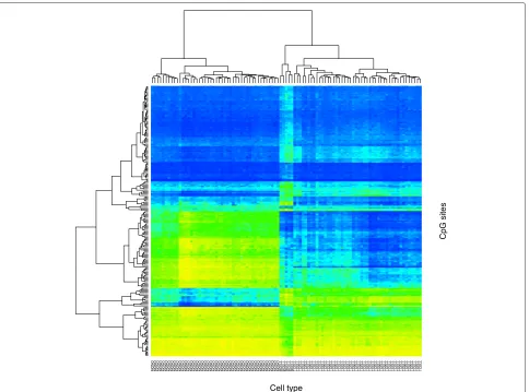
Fig. 1Clustered heat map showing patterns of methylation in 46 SARD samples (columns) and 200 CpG sites (rows). The sites were selected to highlight the methylation differences between cell types. Consequently, the samples cluster by cell type: monocytes, B cells, and then T cells

Multi-layer simulation design

We implemented a rich simulation design, based on the SARD methylation data. This simulation contains ran-dom sources of variability at multiple levels, including both variability of population mean parameters as well as variability at individual-level parameters. Starting with the observed cell-separated methylation profiles for T cells and monocytes from the SARD data, we simulated a number of probes to have associations directly with the phenotype, and we induced confounding by combin-ing the two cell types in proportions that vary across individuals. Although this simulation design is complex and depends on a large number of parameters, it allows substantial flexibility in specifying consistency or variabil-ity between cell types, individuals, or probes, and easily allows us to create realistic and pathological situations in the same framework.

Leti = 1,. . .,nwhere n = 46 denote the individu-als in the SARD data. In brief, the simulation proceeds as follows (see “Methods” for more details):

1. Select a set ofS CpG sites where “true” associations with a phenotype will be generated by our

simulation; we refer to these CpGs as differentially methylated sites (DMSs).

2. Generate a phenotype, either binary (disease or no disease) or continuous.

3. For any probe not in the DMS set, the

cell-type-specific methylation values are the observed values from the real data.

4. For a probe in the DMS set, a randomly generated quantity is added to the observed cell-type-specific level of methylation, in a way that depends on the phenotype.

5. The cell-type-specific methylation values are mixed together in proportions that vary depending on the phenotypes.

types in order to specify an association between change in methylation and cell type. After having specified each of the site- and cell-type-specific associations, we then add between-subject variability to each site. The final step, step 5, leads to methylation proportions as they would appear had the mixed tissue been analyzed directly.

After simulating the data, we then test for associa-tion between the phenotype and the methylaassocia-tion levels in the mixed data at each probe. We compare thepvalues obtained from these tests of association across eight sim-ulation scenarios and eight different methods for cell-type adjustment. Some of the DMSs were simulated to have very small effects and therefore, statistical tests of asso-ciation may not be significant. On the other hand, since the cell-type proportions vary with phenotype, this can lead to non-DMSs showing spurious associations with the phenotype. The notation for the key parameters is given in Table 1, and the parameter choices across different simulation scenarios are summarized in Table 2.

Scenario 1: DMSs have differences in both means and variances between cell types

In our first simulation scenario (Table 2), we chose to specify distinct differences in the strength and distribu-tion of the methyladistribu-tion–phenotype associadistribu-tions (DMS) for the two cell types, with a binary phenotype. Differ-ences in the DMS distributions include both direction of the effects as well as the amount of variability across sites and individuals; Additional file 1: Figure S1 displays his-tograms of the 500 simulated values of the DMS meansμjk for the two cell types, showing the substantial differences between these two distributions.

In this scenario, we would expect that an analysis not taking cell type into consideration should result in many

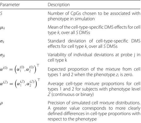
Table 1Fixed parameters in the simulation design

Parameter Description

S Number of CpGs chosen to be associated with phenotype in simulation

μk Mean of the cell-type-specific DMS effects for cell typek, over allSDMSs

σk Standard deviation of cell-type-specific DMS effects for cell typek, over allSDMSs

σjk Variability of individual deviations at probe j in cell type k

α(0)_=α(0) 1 ,α2(0)

Expected proportion of the mixture from cell types 1 and 2 when the phenotypeziis zero.

α(Z)_=α(Z) 1 ,α(2Z)

Average cell-type mixture proportions for cell types 1 and 2 for subjects with phenotype level Z(continuous or binary)

ρ Precision of simulated cell mixture distributions. A greater value corresponds to more clearly defined differences in cell-type proportions with respect to the phenotype

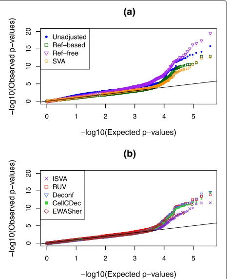
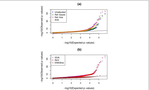
p values that are smaller than expected, or equivalently a greatly inflated slope in a p value QQ plot, due to the strong confounding built into the simulation design. After analyzing for all probes with unadjusted data, we repeated the epigenome-wide analysis with eight popular or newly developed adjustment methods (see “Methods”). QQ plots for these eight methods as well as the uncor-rected analysis can be seen in Fig. 2. Examination of the left-hand side of this plot (x-axis smaller than about 3.5) shows that there is, indeed, a genome-wide inflation of pvalues in the analysis uncorrected for cell-type mixture. Encouragingly, most methods do a fairly good job in cor-recting for the confounding, since the corrected QQ plots are close to the line of expectation up until the tails of each set ofpvalues. The reference-free method, however, continues to display inflation even after correction.

Several numeric performance metrics can be seen in Table 3 for this simulation scenario. One of these met-rics is the genomic inflation factor (GIF) [28], which is the slope of the lines seen in Fig. 2 after removing the 500 DMSs. The unadjusted GIF was 1.6, indicating a substan-tial inflation of significance across allpvalues, but after adjustment most values are quite close to 1.0, as would be expected in the absence of any confounding. The Ref-based, EWASher, and Deconf methods have slopes slightly less than 1.0, implying possible over-correction.

Since we know which 500 sites were generated to be truly DMSs, Table 3 reports both the power and the num-ber of false positives (NFP). We declare a CpG site to be significant if thepvalue falls below the fixed value 10−4_.

This table also shows a measure of performance based on the Kolmogorov–Smirnov (KS) test for whether thep value distribution matches the expected uniform distribu-tion. Of course, the KS test assumes independence of all the individual tests, and therefore, we are not using this test for inference, but simply as a measure of deviation where smaller values imply less deviation.

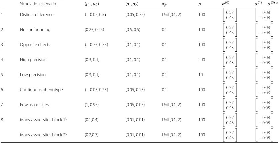
Table 2Parameter choices for the simulation scenarios

Simulation scenario (_μ1,μ2) (σ1,σ2) σjk ρ α(0) α(1)−α(0)a

1 Distinct differences (−0.05, 0.5) (0.05, 0.75) Unif(0.1, 2) 100

0.57 0.43

0.08 −0.08

2 No confounding (0.25, 0.25) (0.5, 0.5) 0.1 100

0.57 0.43

0.08 −0.08

3 Opposite effects (−0.75, 0.75) (0.1, 0.1) 0.1 100

0.57 0.43

0.08 −0.08

4 High precision (0.3, 0.1) (0.1, 0.1) 0.1 200

0.57 0.43

0.08 −0.08

5 Low precision (0.3, 0.1) (0.1, 0.1) 0.1 10

0.57 0.43

0.08 −0.08

6 Continuous phenotype (−0.05, 0.25) (0.05, 0.15) 0.1 100

0.57 0.43

0.03 −0.03

7 Few assoc. sites (1, 0.95) (0.05, 0.05) Unif(0.1, 2) 100

0.57 0.43

0.08 −0.08

8 Many assoc. sites block 1b _{(0.1,0.4) (0.01, 0.01) Unif(0.1, 2) 100}

0.57 0.43

0.08 −0.08

Many assoc. sites block 2c (0.2,0.7) (0.01, 0.01) Unif(0.1, 2) 100

0.57 0.43

0.08 −0.08

k=1 corresponds to monocytes, andk=2 corresponds to CD4+T cells a_{Average change in cell-type proportion for unit increase in phenotype} b_{Background correlation for block 1 was 0.4}

c_{Background correlation for block 2 was 0.5}

to constructing the components, and hence, many DMS probes are not even included in its analyses. Results for the Ref-free power must be interpreted cautiously since the type 1 error is so substantially elevated for this method. The KS statistic confirms the conclusions obtained from other metrics, showing small values for most meth-ods except for the unadjusted data and the Ref-free method.

Scenario 2: no confounding

It is also of interest to examine performance when there is no confounding. By simulating data with the same cell-type-specific means and variances in both cell types (scenario 2 in Table 2), the unadjusted analysis should not be subject to any bias. As expected, Table 4 shows low NFP and good power for the unadjusted method, and similar results are obtained for CellCDec, Deconf, and Ref-based. In Additional file 1: Figure S2, it can be seen that the unad-justed results lie very close to the line of expectation, apart from the tail of the distribution where the DMSs predom-inate. It is interesting to note that SVA, RUV, Ref-free, and in particular ISVA display high NFP, implying that far too many DMS probes are being inferred. Despite that no confounding was simulated, the GIF for the unadjusted data is slightly inflated; in fact, after adjustment, the GIF increases for Ref-free and ISVA. In contrast, the GIF is less than 1 for CellCDec, Deconf, and the Ref-based methods, implying some over-correction.

Scenario 3: opposite effects in different cell types

To investigate a case of severe differential effects, in sce-nario 3, the cell-type-specific meansμk were selected to have opposite signs in the two cell types. In this case, the mixed sample can have small DMS effects, since the two cell-type-specific effects may cancel each other. Con-firming this expectation, there is no inflation of the test statistics in the unadjusted data (GIF=0.97, Table 5). Like the previous scenarios, we see very poor power and over-correction with EWASher, and extremely inflated NFP with the Ref-free method (Additional file 1: Figure S3). Small power improvements over the unadjusted analysis can be seen when using any of the other methods.

Scenarios 4 and 5: altered precision simulations

(b)

0 1 2 3 4 5

0

5

10

15

20

(a)

−log10(Expected p−values)

−log10(Obser

v

ed p−v

alues) Unadjusted Ref−based Ref−free SVA

0 1 2 3 4 5

0

5

10

15

20

−log10(Expected p−values)

−log10(Obser

v

ed p−v

alues) ISVA RUV Deconf CellCDec EWASher

Fig. 2QQ plots showing distributions ofpvalues in simulation

scenario 1 where the true effects in the different cell types have very distinct distributions. Results are shown with no adjustment for cell-type mixture as well as with eight other methods; these are split across two panels, (a) and (b), to clarify the display

In the high-precision scenario, the NFP is extremely high when no adjustment is used. Most methods, how-ever, perform quite well in reducing the GIF and KS statistics, reducing the NFP and retaining decent power (with the exceptions of Ref-free and EWASher as seen pre-viously). In contrast, for the low-precision scenario, where there is much more variability from one individual to the

Table 3Performance metrics under simulation scenario 1 (distinct associations between cell types)

Method Number of false positives Power KS GIF Kˆa

Unadjusted 248 0.208 0.168 1.60 –

Ref-based 14 0.146 0.026 0.92 –

Ref-free 375 0.248 0.097 1.33 13

SVA 32 0.124 0.021 1.05 10

ISVA 14 0.134 0.004 0.97 12

EWASher 3 0.036 0.044 0.92 –

CellCDec 7 0.094 0.008 0.98 –

Deconf 13 0.178 0.023 0.93 –

RUV 36 0.170 0.018 1.04 43

KSKolmogorov–Smirnov statistic,GIFgenomic inflation factor a_{Estimated latent dimension}

Table 4Performance metrics under simulation scenario 2 (no confounding)

Method Number of false positives Power KS GIF Kˆ

Unadjusted 38 0.642 0.059 1.09 –

Ref-based 13 0.594 0.030 0.90 –

Ref-free 366 0.704 0.058 1.25 14

SVA 79 0.646 0.015 1.06 10

ISVA 408 0.654 0.061 1.27 15

EWASher 0 0.126 0.066 0.83 –

CellCDec 14 0.650 0.021 0.93 –

Deconf 50 0.652 0.031 0.92 –

RUV 134 0.640 0.007 1.00 38

KSKolmogorov–Smirnov statistic,GIFgenomic inflation factor

next in the mixture proportions, as well as substantial differences between cases and controls, performance is generally poor. The QQ plots display substantial inflation, and most methods have very high NFP. Even the Ref-based method has very high NFP, and notably the QQ plot for RUV has enormous inflation and with the NFP at 2943. In fact, the unadjusted analysis appears to be one of the bet-ter choices here, with lower NFP and good power; ISVA also seems to perform better than the others.

Scenario 6: continuous phenotype simulation results

In our simulation with continuous phenotypes, the rel-ative performances of the methods are different again. Table 8 and Additional file 1: Figure S6 indicate that unlike all the other scenarios, the Ref-free method performs fairly decently in this case, leading to small reductions in the GIF and KS statistics and a small improvement in power. RUV’s performance is one of the best here, with a low NFP, good power, and an excellent GIF value. In con-trast, the CellCDec method, which had performed quite well in all the other scenarios, shows extensive inflation

Table 5Performance metrics under simulation scenario 3 (opposite effects)

Method Number of false positives Power KS GIF Kˆ

Unadjusted 5 0.490 0.041 0.97 –

Ref-based 1 0.506 0.036 0.87 –

Ref-free 176 0.608 0.053 1.19 14

SVA 37 0.562 0.003 1.00 10

ISVA 49 0.558 0.006 1.01 14

EWASher 0 0.128 0.092 0.74 –

CellCDec 3 0.502 0.033 0.88 –

Deconf 2 0.522 0.035 0.89 –

RUV 23 0.532 0.012 1.00 37

Table 6Performance metrics under simulation scenario 4 (high precision)

Method Number of false positives Power KS GIF Kˆ

Unadjusted 368 0.600 0.142 1.32 –

Ref-based 64 0.460 0.043 1.04 –

Ref-free 437 0.694 0.101 1.36 13

SVA 79 0.534 0.032 1.09 11

ISVA 198 0.522 0.062 1.20 14

EWASher 16 0.072 0.038 0.94 –

CellCDec 54 0.546 0.031 1.05 –

Deconf 58 0.520 0.014 1.02 –

RUV 155 0.568 0.051 1.15 32

KSKolmogorov–Smirnov statistic,GIFgenomic inflation factor

across the QQ plots (GIF=1.44) and a very high NFP. We were unable to obtain results for the Deconf method with three components within the available computa-tional time limits on the Mammouth Compute Canada cluster. We note that the EWASher method does not allow continuous phenotypes and cannot be used in this scenario.

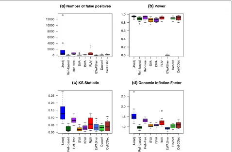
Scenario 7: simulation with a small number of true DMSs

To consider cell-type mixture effects when there are only a few epistable alleles, as has been observed in several stud-ies [29, 30], we created a simulation with only 50 DMSs, exhibiting moderate to strong positive associations with the phenotype in both cell types. Ten replications of the simulation were performed. The parameters in Table 1 were held constant over the different replications, except forσ_jk, which was generated from a uniform distribution to induce some additional variation. Box plots comparing performance over the ten replications can be seen in Fig. 3. QQ plots for all methods under one of the replications can be seen in Additional file 1: Figure S7.

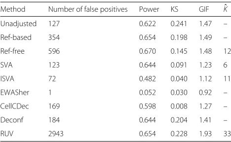
Table 7Performance metrics under simulation scenario 5 (low precision)

Method Number of false positives Power KS GIF Kˆ

Unadjusted 127 0.622 0.241 1.47 –

Ref-based 354 0.654 0.198 1.49 –

Ref-free 596 0.670 0.145 1.48 12

SVA 123 0.644 0.091 1.23 6

ISVA 72 0.482 0.040 1.12 11

EWASher 1 0.052 0.030 0.92 –

CellCDec 169 0.598 0.008 1.27 –

Deconf 184 0.644 0.204 1.41 –

RUV 2943 0.654 0.228 1.93 33

KSKolmogorov–Smirnov statistic,GIFgenomic inflation factor

Table 8Performance metrics under simulation scenario 6 (continuous)

Method Number of false positives Power KS GIF Kˆ

Unadjusted 135 0.532 0.081 1.37 –

Ref-based 13 0.498 0.031 0.99 –

Ref-free 125 0.618 0.061 1.17 14

SVA 29 0.502 0.006 0.99 10

ISVA 114 0.520 0.076 1.21 14

CellCDec 422 0.420 0.079 1.44 –

Deconfa _{– – – – –}

RUV 16 0.550 0.006 0.966 39

KSKolmogorov–Smirnov statistic,GIFgenomic inflation factor

a_{No results were obtained withK=3 in the allowable time on the computational} cluster Mammouth

Unsurprisingly, the performance metrics are quite vari-able when the analysis does not adjust for cell-type com-position. The NFP of both the reference-free method and RUV vary substantially. In contrast, both the reference-based and SVA methods show a very good reduction in the number of non-DMSs below this p value threshold across all replications. Most methods do not achieve a power as high as the unadjusted method; however, the lowered NFP is a worthy tradeoff for the loss in power, especially for the reference-based and SVA methods. Most methods improve the KS statistic and GIF, except for the reference-free method, which has values almost as high as those in the unadjusted analysis.

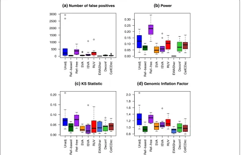
Scenario 8: widespread, subtle, correlated DMS effects

In the final simulation scenario, we simulated a large num-ber of associated DMSs to capture the possibility of a subtle genome-wide shift in methylation, such as might be seen for a large change in metabolic functioning or in immune system function. Here, we randomly selected 10,000 CpG sites to be DMSs, and unlike the previous simulation scenarios, we created dependence between the phenotype-associated methylation shifts at these sites. The DMSs were grouped into two blocks of size 5000, and a moderate background level of correlation between the mean effect sizes μjk was included in each block. Effect sizes across blocks were still generated indepen-dently. Additional details of the dependence structure can be seen in step 4 of the “Methods” section, and the param-eter choices can be seen in Table 2. Box plots comparing performance over the ten replications are shown in Fig. 4. QQ plots for all methods under one of the replications can be seen in Additional file 1: Figure S8.

Unadj

Ref−based Ref−free

SV

A

ISV

A

RU

V

EW

ASher _Deconf

CellCDec

CellCDec CellCDec

CellCDec

0 2000 4000 6000 8000 10000 12000

(a) Number of false positives

Unadj

Ref−based Ref−free

SV

A

ISV

A

RU

V

EW

ASher _Deconf

0.0 0.2 0.4 0.6 0.8 1.0

(b) Power

Unadj

Ref−based

Ref−free

SV

A

ISV

A

RU

V

EW

ASher _Deconf

0.00 0.05 0.10 0.15 0.20 0.25

(c) KS Statistic

Unadj

Ref−based

Ref−free

SV

A

ISV

A

RU

V

EW

ASher _Deconf

1.0 1.5 2.0 2.5

(d) Genomic Inflation Factor

Fig. 3Comparison of performance metrics over ten replications in Scenario 7, few associated DMS.aThe number of non-differentially methylated

sites with a rawpvalue less than 10−4_{.bPower at significance level 10}−4_{.cKolmogorov–Smirnov statistic.dGenomic inflation factor}

perform well in this scenario. Power is lower in all meth-ods compared to the other simulation scenarios, with the exception of the reference-free method, though the high NFP for that method undermines this result. Most methods perform fairly similarly when considering the KS statistic and GIF.

Estimated latent dimension

Our simulation is based on complex mixtures of methyla-tion profiles from two separated cell types. It is, therefore, interesting to note that for all the methods that provide estimates for the latent dimension (the last column of Tables 3, 4, 5, 6, 7 and 8), these estimates are consis-tently much larger than 2. Estimates are obtained for the Ref-free, SVA, ISVA, and RUV methods. Both SVA and ISVA assume the number of surrogate variables is less than or equal to the number of true confounders whose linear space they span, and for RUV, the authors them-selves commented that the estimated values for K do not necessarily reflect the true dimension [27]. All esti-mates are generally greater than ten, and RUV’s estiesti-mates tend to be over 30. In fact, there may be some additional sources of variation present in the original cell-separated

methylation data, and these factors are likely being cap-tured by these numerous latent variables. In fact, analy-ses of the original cell-type-separated data using patient age as the predictor resulted in estimated latent dimen-sions that were themselves large. For example, random matrix theory [31] (which is used for dimension estima-tion in the reference-free method and ISVA) estimated a latent dimension of ten for both T cells and monocytes when analyzed separately. Furthermore, SVA estimated the number of surrogate variables to be seven and nine for T cell and monocytes, respectively.

Results from analysis of the ARCTIC data set

Unadj

Ref−based

Ref−free

SV

A

ISV

A

RU

V

EW

ASher _Deconf

CellCDec

CellCDec CellCDec

CellCDec

0 500 1000 1500 2000 2500 3000

(a) Number of false positives

Unadj

Ref−based

Ref−free

SV

A

ISV

A

RU

V

EW

ASher _Deconf

0.00 0.05 0.10 0.15 0.20 0.25 0.30

(b) Power

Unadj

Ref−based

Ref−free

SV

A

ISV

A

RU

V

EW

ASher _Deconf

0.00 0.05 0.10 0.15 0.20

(c) KS Statistic

Unadj

Ref−based

Ref−free

SV

A

ISV

A

RU

V

EW

ASher _Deconf

0.8 1.0 1.2 1.4 1.6 1.8 2.0

(d) Genomic Inflation Factor

Fig. 4Comparison of performance metrics over ten replications in the many associated DMSs scenario.aNumber of non-differentially methylated

sites with a rawpvalue less than 10−4_{.bPower at significance level 10}−4_{.cKolmogorov–Smirnov statistic.dGenomic inflation factor}

(473,864 probes). We excluded the colorectal cancer patients from this analysis due to concerns that their methylation profiles may have been affected by treat-ment. Patient age was included as a covariate in all analyses.

Figure 5 shows the QQ plots for seven adjustment meth-ods, and Table 9 provides KS and GIF numeric metrics of performance. The Deconf and CellCDec methods could not be used with these data since the computational time exceeded the 5-day limit allowed on the Mammouth clus-ter of Calcul Quebec. As was seen in our simulations, the EWASher method seems to over-correct, leaving no sig-nificant probes, and the GIF is much smaller than 1.0. However, all other methods lead to QQ plots where the slope is larger after correction than before; the GIF esti-mates are substantially larger than for the unadjusted analysis. For SVA and ISVA, the KS statistic is increased after corrections are applied. Furthermore, among the top 1000 probes selected by each method (based on raw p value), none were shared by all methods (including unad-justed results). If EWASher was excluded, 87 probes over-lapped among the most significant 1000, and 89 probes overlapped among methods excluding EWASher and the

unadjusted results. Therefore, the methods are highlight-ing quite different results for the most significant probes.

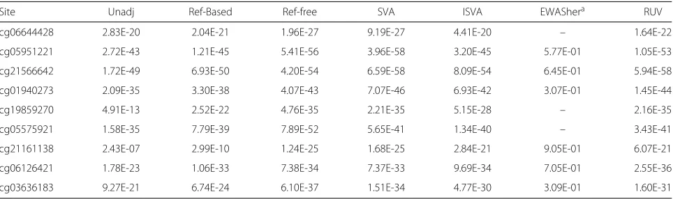
In Table 10,pvalues are shown for probes that have been linked to smoking status in a large published EWAS [33]. They specifically discuss seven CpGs, previously reported as associated with smoking, that were replicated in their work. Although substantial evidence of association can be seen at all probes, it is interesting to see the differences in significance across methods. For example, at probe cg21161138, significance ranges from 10−7to 10−25.

Results from analysis of the rheumatoid arthritis data set

0 1 2 3 4 5

01

0

3

0

5

0

(a)

−log10(Expected p−values)

−log10(Obser

v

ed p−v

alues) Unadjusted Ref−based Ref−free SVA

0 1 2 3 4 5

01

0

3

0

5

0

(b)

−log10(Expected p−values)

−log10(Obser

v

ed p−v

alues) ISVA RUV EWASher

Fig. 5QQ plots of₋log₁₀pvalues from the ARCTIC study with different adjustment methods. These are split across two panels, (a) and (b), to clarify

the display

We attempted to replicate the original analysis as closely as possible by using the Illumina control probe scaling procedure, including the same covariates in our linear model (age, sex, and smoking status), and adjusting for cell-type composition using the reference-based method. However, when extracting the significant CpGs men-tioned in their Additional file 1, the distribution of rawp values in our analysis did not match those in the original paper. This could suggest there is a step in the origi-nal aorigi-nalysis not explicitly stated in the paper’s “Methods” section. However, since for our purposes, we wish to compare the results of the adjustment methods relative

Table 9Performance metrics for the ARCTIC data with the most significant probes removed (top 5 %)

Method KS statistic GIF Kˆ

Unadjusted 0.0758 0.9142 –

Ref-based 0.0508 0.9907 –

Ref-free 0.0296 1.1499 32

SVA 0.0362 1.0962 15

ISVA 0.1208 1.6820 39

EWASher 0.7291 1.0164 –

RUV with three components 0.0906 1.2423 –

It was not possible to obtain results for the CellCDec and Deconf methods KSKolmogorov–Smirnov statistic,GIFgenomic inflation factor

to each other, we do not believe this to be a significant issue. For our comparison, we have used functional nor-malization [35]. Comparisons of the distribution of the reportedpvalues and the ones we obtained can be seen in Additional file 1: Figure S9.

The results from our analysis are summarized in Fig. 6. We performed the cell-type adjustment methods using all probes on autosomes, but restricted the analysis to the 51,478 probes reported in the paper. We examine the pro-portion of CpGs present in the top d significant CpGs found in each method that were also present in the top dCpGs found in the original paper. The method showing the highest concordance with the originally reported CpG list is the reference-based method, which was expected given that the reference-based method was used in the original analysis. It is evident, however, that the different adjustment methods do not replicate the findings of the original study, especially for smaller values ofd. We have shown that the choice of cell-type adjustment method can drastically change the conclusions of an EWAS.

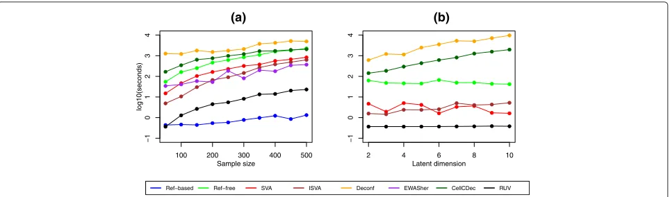
Computational performance

Table 10Pvalues for sites previously found to be associated with smoking [33]

Site Unadj Ref-Based Ref-free SVA ISVA EWAShera _RUV

cg06644428 2.83E-20 2.04E-21 1.96E-27 9.19E-27 4.41E-20 – 1.64E-22

cg05951221 2.72E-43 1.21E-45 5.41E-56 3.96E-58 3.20E-45 5.77E-01 1.05E-53

cg21566642 1.72E-49 6.93E-50 4.20E-54 6.59E-58 8.09E-54 6.45E-01 5.94E-58

cg01940273 2.09E-35 3.30E-38 4.07E-43 7.07E-46 6.93E-42 3.07E-01 1.45E-44

cg19859270 4.91E-13 2.52E-22 4.76E-35 2.21E-35 5.15E-28 – 2.16E-35

cg05575921 1.58E-35 7.79E-39 7.89E-52 5.65E-41 1.34E-40 – 3.43E-41

cg21161138 2.43E-07 2.99E-10 1.24E-25 1.68E-25 2.84E-21 9.05E-01 6.07E-21

cg06126421 1.78E-23 1.06E-33 7.38E-34 7.37E-33 9.69E-34 7.05E-01 2.55E-36

cg03636183 9.27E-21 6.74E-24 6.10E-37 1.51E-34 4.77E-30 3.09E-01 1.60E-31

a_{Several sites were filtered out by EWASher}

any statistical inference here, all samples were included, regardless of whether we had matching cell-type sets or quality control status. Some of the methods calculate pvalues and parameter estimates internally, and others require the use of an external function to perform a linear fit. Therefore, to make the computational times compa-rable, we define the start time as when the adjustment method is first called, and the end time when all estimates andpvalues have been obtained.

Figure 7 shows the running times on the log scale, as the sample size increases (N = 50 to N = 500), and for methods where a value of the latent dimensionKcan be specified, running times asK increases with a fixed sample size (N = 50). There are major differences in running times for the cell-type adjustment methods. Not surprisingly, the Ref-based method is very fast, as is RUV.

0 2000 4000 6000 8000 10000

0.0

0

.1

0.2

0

.3

0.4

0.5

0.6

Number of top CpGs considered (d)

Propor

tion in or

iginal list

Ref−based Ref−free SVA ISVA CellCDec EWASher RUV

Fig. 6Agreement of the proportion of topdCpGs declared

significant in the different cell-type adjustment methods with the top dCpGs in the originally reported list of significant CpGs from the rheumatoid arthritis study

The slowest methods are Deconf and CellCDec. The com-putational time required for the Ref-free method also increases quickly with the sample size. In Fig. 7b, it is interesting to note that increasingKhas very little effect on the speed of four of the six methods that require a specification ofK. However, the computational times for both CellCDec and Deconf increase exponentially with larger values ofK. As noted previously, we were not able to obtain results for these methods with the ARCTIC data set when using all autosomal probes. We note also that the complexity of preparation of the input files also varies from one algorithm to another.

Discussion

We have presented an extensive comparison of eight different methods for adjusting for cell-type-mixture confounding, by designing a rich simulation based on cell-type-separated methylation data in SARD patients. Our simulation contained multiple levels of variability, between cell types, at the level of the probe means, and at the level of the individual. We found that there was no adjustment method whose performance was uniformly the best, and in fact in some of our scenarios, the unad-justed results were quite comparable to the best adunad-justed results. These general conclusions were similar whether we had a few DMSs of large effect (scenario 7) or many correlated DMSs of smaller effect size (scenario 8).

100 200 300 400 500

−1

0

123

4

(a)

Sample size

log10(seconds)

2 4 6 8 10

−1

0

123

4

(b)

Latent dimension

Ref−based Ref−free SVA ISVA Deconf EWASher CellCDec RUV

Fig. 7Computational time comparison.aSample size. The latent dimension was estimated by the algorithms as needed.bLatent dimension. The

sample size is fixed at 50

designing the simulation setup and choosing parameter values.

In many of our simulated scenarios, as might be expected, the reference-based method performed well. This method is very easy to implement, and as seen in the computing performance section, it runs very quickly, even on larger sample sizes. It usually achieved good statistical power, and, with one exception, reduced NFP relative to the unadjusted model. It also has the advantage of being able to estimate directly the cell-type composition of each sample. Therefore, the Ref-based method is an obvious choice when a complete set of the required cell-separated methylation profiles are available; however, this is not always the case. For some tissues, cell types that are of par-ticular interest are very difficult or impossible to extract; one example here would be the syncytiotrophoblast cells in placenta [36, 37].

In every case we examined, EWASher did a very good job in reducing p value inflation, and GIF values were substantially reduced from the unadjusted analyses. How-ever, that this method so strictly forces the GIF factor downwards may raise concerns about over-correction. If there were, for example, global hypermethylation associ-ated with a disease, adjustment using EWASher would be overly conservative. Additionally, part of the algorithm involves filtering out loci that are unilaterally high or low among all subjects. The assumption behind this filter is that these loci are, for all intents and purposes, com-pletely methylated or unmethylated and any associations between these probes and the phenotype are not interest-ing. This may be an overly strong assumption. In our sim-ulations, this filter results in the dramatically worse power of this method, since we did not restrict the randomly selected DMS loci to any particular mean level of methy-lation. Furthermore, the EWASher method is quite diffi-cult to implement. Although most methods can be run in R (https://www.r-project.org), EWASher requires the

user to create three separate input files for a standalone executable, and then to perform post-processing in R.

We cannot explain the poor performance in our sim-ulations of the Ref-free method. The NFP were almost always more inflated than in the raw data, and this infla-tion is clearly visible in the QQ plots. Furthermore, the implementation was somewhat more complex since the approach involved one step to estimate the latent dimen-sion, a second to get parameter estimates, and then finally bootstrap calculations to obtain standard errors. The per-formance of the Ref-free method was good for scenario 6 with a continuous phenotype, so we hypothesize that there are some linearity assumptions in the correction that are being violated in our binary phenotype simulations.

and is available as an R function. It contains a function to estimate the latent dimension (K), although, akin to the other methods that estimateK, the estimated dimen-sion tends to be much higher than the simulated reality. We performed some investigations into how RUV per-forms at a range of values forK, and the best performance was observed, in most simulation scenarios, at smaller values such as K = 3. Recently, Houseman also found that estimated latent dimensions obtained through ran-dom matrix theory may not be the best choices [38]. RUV is also extremely fast, slower only than the Ref-based method, and as shown in Fig. 7, the computational time is essentially invariant as the latent dimension is varied, making this an attractive option. Nevertheless, the SVA method, although rarely the best, did not have any notable failures across our scenarios, and was easy to implement.

There are other methods for deconvolution that we did not examine, especially in the computer science and engi-neering literature [39]. However, it is not clear whether these methods would be easily adapted for use on methy-lation data. Also, new methods for DNA methymethy-lation analysis continue to be published, such as [40]. However, the spectrum of methods that we have examined includes the most-commonly used approaches. All methods that we have examined assume approximately linear relation-ships between the phenotype and the methylation levels or covariates; however, this should not be an important limitation since approximate linearity should hold [38].

The latent dimension, when estimated, was rarely simi-lar to the dimension ofK=2 implemented in our simula-tion. However, these estimates ofKcapture aspects of het-erogeneity in the data that are only partially attributable to the mixture of data from two cell types. This hetero-geneity may also be partially due to technological artefacts from batch effects or experimental conditions, and in par-ticular to the fact that subtler cell lineage differences will still be present even after cell sorting [38].

In summary, our simulation study comparing methods found a wide range of performance across our scenarios with notable failures of some methods in some situations. We recommend SVA as a safe approach for adjustment for a cell-type mixture since it performed adequately in all simulations with reasonable computation time. In all situations, EWAS results are extremely sensitive to the normalization and cell-type adjustment methods used, and hence, this issue should receive more attention when interpreting findings.

A set of scripts enabling implementation of all these methods can be found at https://github.com/ GreenwoodLab/CellTypeAdjustment.

Conclusions

We have compared eight different methods for adjusting methylation data for cell-type-mixture confounding in a

rich and multi-layered simulation study, and in a large set of samples where methylation was measured in whole blood. No method performs best in all simulated scenar-ios, nevertheless we recommend SVA as a method that performed adequately without notable failures.

Methods

Patient data and quality checks

Ethical approval was obtained at the Jewish General Hos-pital and at McGill University, Montreal, QC, to obtain whole-blood samples from the patients with SARDs, at the time of initial diagnosis prior to any treatment. Cell purification and phenotyping protocols for cell subset isolation, analysis, purity evaluation, fractionation, and storage were standardized and optimized. Then 40 ml of peripheral blood were obtained from the above subjects and processed within 4 hours. PBMCs were separated with lymphocyte separation medium (Mediatech, Inc.). Isolated PBMCs were sequentially incubated with anti-CD19, anti-CD14, and anti-CD4 microbeads (Miltenyi Biotec). Automated cell separation of specific cell subpop-ulations was performed with auto-MACS using positive selection programs. An aliquot of the specific isolated cell subtypes was used for purity assessment with flow cytometric analysis. A minimum of 2 million cells from each subpopulation with a purity higher than 95 % were frozen in liquid nitrogen for the epigenomic studies. The optimized protocols required the isolation of sufficient numbers of CD4+ lymphocytes (9.04±4.03×106) and CD14+monocytes (7.89±2.96×106), and CD19+B lym-phocytes (2.02±1.42×106_{), of sufficient purity to perform}

the epigenetic analyses.

The required number of cells with the right purity was not always available, especially for the CD19+ B lym-phocytes, so we did not have all three cell types for all patients; for this reason, the simulation used only two cell types and 46 patients. Illumina Infinium HumanMethy-lation450 BeadChip data were normalized with funnorm [35]. Also, a number of probes were removed, specifi-cally those on the sex chromosomes as well as probes close to single-nucleotide polymorphisms [41]. There were 375,639 probes remaining after filtering.

Details of the simulation method

This simulation design was initially developed in the mas-ter’s thesis of the first author [42].

1. Selection of DMS probes:S=500probes were randomly selected to be associated with the phenotype.

2. Phenotype (zi,i=1,. . .,n): A random sample of size

3. Cell-type-specific methylation values for non-DMS probes: Letβijkrepresent the true methylation value

for individuali, probe j, and cell type k. For a probe that is not a DMS probe, the simulated value β

ijk=βijk.

4. Cell-type-specific methylation values for DMS probes:

• Cell-type-specific means are sampled from normal distributions with given parameters. That is, for chosen valuesμkandσkfork=1, 2,

cell-type-specific means that for each DMS probe,μjkare generated fromμjk∼N

μk,σ_k2

. In scenario 8, we split the DMSs into two blocks and simulate effect sizes from a multivariable normal distribution with a fixed background correlation in each block. That is, probes in the same block are correlated, but probes across blocks are independent from one another. In this scenario, the parametersμkfork=1, 2

differ between the blocks.

• The simulated cell-type-specific methylation effect,_ijk, at a DMS, for an individual samplei and an individual probej, is another random quantity, so that

e_ijk ∼Nμ_jk,σ_jk2

whereσjkis a parameter provided to the

simulation.

• For either a binary or continuous phenotypezi,

the simulated methylation valueβijkis then

β

ijk=logit−1

logitβijk

+zieijk

.

Although all the random effects were simulated on a linear scale, the results are reconverted to the (0,1) scale since several of the cell-type adjustment methods require this range.

5. Combining across cell types:

• Each individual is assumed to have a unique mixture of the two cell types in a way that depends on the phenotype,z. Let

α(0)_=α(0) 1 ,α(20)

represent the average proportions of the two cell types whenzi=0,

and then letα(Z)_=α(Z)

1 ,α

(Z) 2

be these proportions whenzi=Z. We then say,

α(Z)_=α(0)_+Z

×

average change in proportion in monocytes average change in proportion in T cells

.

(1)

• The cell-type proportionspikfor individuali

were then generated from Dirichletρα_k(Z), whereρ >0is a precision parameter, such that larger precision corresponds to less variation in the observed values.

• The final simulated beta value for personi at CpG sitej becomes

βf

ij=pi1βij1+pi2βij2. (2)

Key notation definitions are summarized in Table 1, and parameter choices for the simulations are in Table 2.

Description of adjustment methods

The performance of eight popular methods is compared. Brief descriptions of each method are provided here, and Table 11 compares some key features of the methods, including some details of the implementations. This set of eight methods is not an exhaustive list of all methods available at this time. In fact, in other fields, particu-larly engineering and computer science, there exists a plethora of other methods under the guise of deconvo-lution providing the same kind of correction for unmea-sured confounding in other high-throughput data sources [39]. However, we include and compare many of the approaches that are in common usage in the last few years in the world of genomics and epigenomics.

Reference-based

This method was published in 2012 by Houseman et al. [19]. It relies on the existence of a separate data set containing methylation measurements on separated cell types. The method uses methylation profiles for the indi-vidual cell types to estimate directly the cell-type compo-sition of each sample. However, cell-separated data are not always available for all constituent cell types.

Reference-free

The second method from Houseman et al. does not depend on a reference data set, and therefore, can be used in methylation studies on any tissue type [20]. Rather than directly estimating cell-type composition, the reference-free method performs a singular value decomposition on the concatenation of the estimated coefficient and resid-ual matrices from an initial, unadjusted model. A set of latent vectors is then obtained that accounts for cell type in further analyses.

Surrogate variable analysis

Table 11Comparison of some features of the methods for cell-type mixture adjustment

Method Phen. alloweda _{Input values}b _Kc _Link

Ref-based Any Beta N/A http://people.oregonstate.edu/~housemae/software/TutorialLondon2014

http://bioconductor.org/packages/release/bioc/html/minfi.html

Ref-free Any Beta Estimated http://cran.r-project.org/web/packages/RefFreeEWAS/index.html

SVA Any Beta or logit(beta) Estimated http://bioconductor.org/packages/release/bioc/html/sva.html

ISVA Continuous Beta or logit(beta) Estimated http://cran.r-project.org/web/packages/isva/index.html

EWASher Binary Beta Estimated http://research.microsoft.com/en-us/downloads/472fe637-7cb9-47d4-a0df-37118760ccd1

CellCDec Not used Beta Input https://github.com/jameswagner/CellCDec

Deconf Not used Beta or logit(beta) Input http://web.cbio.uct.ac.za/~renaud/CRAN

RUV Any Beta or logit(beta) Estimated https://cran.r-project.org/web/packages/ruv/index.html

a_{What kinds of phenotype are allowed?}

b_{Does the method use methylation proportions (beta values)? Or logit transformed beta values?} c_{Does the method estimate the number of latent cell typesK, or isKinput into the algorithm?}

It is based on a singular value decomposition on the resid-ual matrix from a regression model not accounting for cell-type composition. The total number of surrogate vari-ables included in the model is based on a permutation test.

Independent surrogate variable analysis

Independent surrogate variable analysis (ISVA) from Teschendorff et al. [24] is very similar in principle to SVA. The main difference is that instead of applying singular value decomposition, it uses independent com-ponent analysis (ICA), which attempts to find a set of latent variables that are as statistically independent as possible.

FaST-LMM-EWASher (EWASher)

This method from Zou et al. [22] extends the Factored Spectrally Transformed Linear Mixed Model algorithm (FaST-LMM) [43] for use in the context of EWAS. A sim-ilarity matrix is calculated based on the methylation pro-files, and principal components are subsequently included in the linear mixed model until GIF is controlled. The maximum number of principal components allowed was fixed as ten.

Removing unwanted variation

The method called Removing Unwanted Variation (RUV) was published in 2012 [26] by Gagnon-Bartsch and Speed. It performs a factor analysis on negative control probes to separate out variation due to unmeasured confounders, while leaving the variation due to the factors of interest intact. Here we use RUV-4, an extension to the original published version, which uses elements from RUV as well as SVA [27]. Control probes were chosen from a list of 500 probes on the 450K platform known to be differen-tially methylated with blood cell type and age [13]. We selected probes that were not strongly correlated with the simulated phenotype.

Deconfounding

The Deconf method from Repsilber et al. [25] was devel-oped for gene expression studies on heterogeneous tissue samples, but is applicable for use in EWAS. The algo-rithm performs a non-negative matrix factorization on the methylation matrix, but does not consider the phenotype in correcting for the heterogeneity and does not estimate the number of cell types present.

CellCDec

CellCDec was developed by Wagner [21], and is sim-ilar to Deconf in that it does not consider the phe-notype in performing its decomposition and does not internally estimate the number of cell types present. The method assumes a specific regression parameterization, and makes random perturbations to the model parame-ters, which are accepted if there is a decrease in the sum squared residuals.

Additional statistical details

For each of the simulation scenarios 1–6, the simulation was run once, whereas in scenarios 7 and 8, we per-formed ten replications. DMSs were chosen randomly in each simulation scenario and within each replication. After cell-type adjustment, a linear model was performed including the latent variables as covariates (except in EWASher where the model was run within the function call). Standard errors were obtained after performing the empirical Bayes methodeBayesfrom thelimma pack-age in R. Probes were declared significant if thepvalue fell below the fixed value 10−4.

For SVA, we used the “iteratively re-weighted least squares” option; however, no control probes were speci-fied. For RUV, the control probes were chosen from sites previously shown to be associated with blood cell type and age, but were not significantly associated with the pheno-type of interest, a necessary condition for a probe to be used as a control in this method.

For each of the methods requiring a pre-specified value ofK, the latent dimension, we ran the methods multiple times with different values of K. We consistently found that performance did not change with increasing values of K and so when running the methods CellCDec and Deconf, the value ofK was fixed at 3 in all scenarios to keep running times down. For the RUV method, we also noticed better performance whenKwas fixed at 3, despite that the method consistently estimated a much higher value for that parameter. All results shown for RUV were run withKfixed at 3.

None of the other adjustment methods had specific options or tuning parameters that needed to be provided by the user.

Compliance with ethical standards

Ethics committee approval for this study was obtained at McGill University and all subjects provided informed written consent to participate in the study. The Institu-tional Research Board (IRB) number is [A12 M83 12A]. This study complies with the Helsinki Declaration.

Availability of supporting data

The data sets supporting the results of this article are available in the repositories:

1. ARCTIC data are in dbGAP under accession number [phs000779.v1.p1], http://www.ncbi.nlm.nih.gov/ projects/gap/cgi-bin/study.cgi?study_id=phs000779. v1.p1.

2. The rheumatoid arthritis data are available under accession number [GSE42861], https://www.ncbi. nlm.nih.gov/geo/query/acc.cgi?acc=GSE42861. 3. Data for simulation scenarios for cell-type mixtures

are available at Zenodo [10.5281/zenodo.46746], https://zenodo.org/record/46746#.VtW8H2SAOko.

Additional file

Additional file 1: Contains plots showing simulated effect sizes among 500 CpGs in simulation scenario 1, and QQ plots forpvalues of several simulation scenarios. (PDF 771 kb)

Competing interests

The authors declare that they have no competing interests.

Authors’ contributions

Study design: KM, AL, CG. Data collection: MH, SB, IC, TP. Data analysis: KM. Writing manuscript: KM, AL, CG, MH. All authors read and approved the final manuscript.

Acknowledgments

Computations were made on the supercomputer Mammouth parallèle 2 from Université de Sherbrooke, managed by Calcul Québec and Compute Canada. The operation of this supercomputer is funded by the Canada Foundation for Innovation (CFI), NanoQuébec, RMGA, and the Fonds de recherche du Québec, Nature et technologies (FRQ-NT).

Funding

This work was funded by the Ludmer Centre for Neuroinformatics and Mental Health, by the Canadian Institutes of Health Research operating grant MOP-300545, and by a Lady Davis Institute Clinical Research Pilot Project award.

Author details

1_{McGill University, Department of Epidemiology, Biostatistics, and} Occupational Health, 1020 Pine Ave. West, H3A 1A2 Montréal, QC, Canada. 2_{Lady Davis Research Institute, Jewish General Hospital, 3755 Chemin de la} Côte Sainte Catherine, H3T 1E2 Montréal, QC, Canada.3_{Division of} Rheumatology, Jewish General Hospital, Montréal, QC, Canada.4McGill University and Genome Quebec Innovation Centre, McGill University, Montréal, QC, Canada.5Department of Human Genetics, McGill University, Montréal, QC, Canada.6_{Department of Medicine, McGill University, Montréal, QC, Canada.} 7_{The Research Institute of the McGill University Health Centre, Montréal, QC,} Canada.8_{Department of Psychiatry, McGill University, Montréal, QC, Canada.} 9_{The Douglas Mental Health University Institute, Verdun, QC, Canada.}

Received: 1 March 2016 Accepted: 5 April 2016

References

1. Choy MK, Movassagh M, Goh HG, Bennett MR, Down TA, Foo RS. Genome-wide conserved consensus transcription factor binding motifs are hyper-methylated. BMC Genom. 2010;11(1):519.

2. Rakyan V, Down T, Balding D, Beck S. Epigenome-wide association studies for common human diseases. Nat Rev Genet. 2011;12(8):529–41. 3. Khavari DA, Sen GL, Rinn JL. DNA methylation and epigenetic control of

cellular differentiation. Cell Cycle. 2010;9(19):3880–3.

4. Meissner A, Mikkelsen TS, Gu H, Wernig M, Hanna J, Sivachenko A, et al. Genome-scale DNA methylation maps of pluripotent and differentiated cells. Nature. 2008;454(7205):766–70.

5. Bird A. DNA methylation patterns and epigenetic memory. Genes Dev. 2002;16:6–21.

6. Laird P. Principles and challenges of genome-wide DNA methylation analysis. Nat Rev Genet. 2010;11:191–203.

7. Farid N. The immunogenetics of autoimmune diseases. Boca Raton, FL: CRC Press; 1991.

8. Papp G, Horvath I, Barath S, Gyimesi E, Spika S, Szodoray P, et al. Altered T-cell and regulatory cell repertoire in patients with diffuse cutaneous systems sclerosis. Scand J Rheumatol. 2011;40:205–10.

9. Gambichler T, Tigges C, Burkert B, Hoxtermann S, Altmeyer P, Kreuter A. Absolute count of T and B lymphocyte subsets is decreased in systemic sclerosis. Eur J Med Res. 2010;15:44–6.

10. Wagner D, Kaltenhauser S, Pierer M, Wilke B, Arnold S, Hantzschel H. B lymphocytopenia in rheumatoid arthritis is associated with the DRB1 shared epitope and increased acute phase response. Arthritis Res. 2002;4(4):R1.

11. Manda G, Neagu M, Livescu A, Constantin C, Codreanu C, Radulescu A. Imbalance of peripheral B lymphocytes and NK cells in rheumatoid arthritis. J Cell Mol Med. 2003;7(1):79–88.

12. Scott D, Wolfe F, Huizinga T. Rheumatoid arthritis. Lancet. 2010;376(9746):1094–108.

13. Jaffe A, Irizarry R. Accounting for cellular heterogeneity is critical in epi-genome-wide association studies. Genome Biol. 2014;15:R31. 14. Reinius L, Acavedo N, Joerink M, Pershagen G, Dahlen SE, Greco D, et al.

Differential DNA methylation in purified human blood cells: implications for cell lineage and studies on disease susceptibility. PLoS One. 2012;7(7): e41361.

16. Liang L, Cookson W. Grasping nettles: cellular heterogeneity and other confounders in epigenome-wide association studies. Hum Mol Genet. 2014;21(R1):83–8.

17. Liu Y, Aryee M, Padyukov L, Fallin M, Hesselberg E, Runarsson A, et al. Epigenome-wide association data implicate DNA methylation as an intermediary of genetic risk in rheumatoid arthritis. Nat Biotechnol. 2013;31(2):142–8.

18. Michels K, Binder A, Dedeurwaerder S, Epstein C, Greally J, Gut I, et al. Recommendations for the design and analysis of epigenome-wide association studies. Nat Methods. 2013;10(10):940–55.

19. Houseman EA, Accomando WP, Koestler DC, Christensen BC, Marsit CJ, Nelson HH, et al. DNA methylation arrays as surrogate measures of cell mixture distribution. BMC Bioinform. 2012;13(1):86.

20. Houseman EA, Molitor J, Marsit CJ. Reference-free cell mixture adjustments in analysis of DNA methylation data. Bioinformatics. 2014;30(10):1431–9.

21. Wagner J. Computational approaches for the study of gene expression, genetic and epigenetic variation in human. Montreal, QC: McGill University School of Computer Science; 2015.

22. Zou J, Lippert C, Heckerman D, Aryee M, Listgarten J. Epigenome-wide association studies without the need for cell-type composition. Nat Methods. 2014;11(3):309–11.

23. Leek JT, Storey JD. Capturing heterogeneity in gene expression studies by surrogate variable analysis. PLoS Genet. 2007;3(9):e161.

24. Teschendorff AE, Zhuang J, Widschwendter M. Independent surrogate variable analysis to deconvolve confounding factors in large-scale microarray profiling studies. Bioinformatics. 2011;27(11):1496–505. 25. Repsilber D, Kern S, Telaar A, Walzl G, Black GF, Selbig J, et al. Biomarker

discovery in heterogeneous tissue samples-taking the in-silico deconfounding approach. BMC Bioinform. 2010;11(1):27. 26. Gagnon-Bartsch JA, Speed TP. Using control genes to correct for

unwanted variation in microarray data. Biostatistics. 2012;13(3):539–52. 27. Gagnon-Bartsch JA, Jacob L, Speed TP. Removing unwanted variation

from high dimensional data with negative controls. Berkeley: Department of Statistics. University of California; 2013.

28. Devlin B, Roeder K. Genomic control for association studies. Biometrics. 1999;55:997–1004.

29. Harris RA, Nagy-Szakal D, Kellermayer R. Human metastable epiallele candidates link to common disorders. Epigenetics. 2013;8(2):157–63. 30. Silver MJ, Kessler NJ, Hennig BJ, Dominguez-Salas P, Laritsky E, Baker

MS, et al. Independent genomewide screens identify the tumor suppressor VTRNA2-1 as a human epiallele responsive to periconceptional environment. Genome Biol. 2015;16(1):118. 31. Plerou V, Gopikrishnan P, Rosenow B, Amaral LAN, Guhr T, Stanley HE.

Random matrix approach to cross correlations in financial data. Phys Rev E. 2002;65(6):066126.

32. Zanke BW, Greenwood CM, Rangrej J, Kustra R, Tenesa A, Farrington SM, et al. Genome-wide association scan identifies a colorectal cancer susceptibility locus on chromosome 8q24. Nat Genet. 2007;39(8):989–94. 33. Tsaprouni LG, Yang TP, Bell J, Dick KJ, Kanoni S, Nisbet J, et al. Cigarette smoking reduces DNA methylation levels at multiple genomic loci but the effect is partially reversible upon cessation. Epigenetics. 2014;9(10): 1382–96.

34. Liu Y, Aryee MJ, Padyukov L, Fallin MD, Hesselberg E, Runarsson A, et al. Epigenome-wide association data implicate DNA methylation as an intermediary of genetic risk in rheumatoid arthritis. Nat Biotechnol. 2013;31(2):142–7.

35. Fortin JP, Labbe A, Lemire M, Zanke BW, Hudson TJ, Fertig EJ, et al. Functional normalization of 450k methylation array data improves replication in large cancer studies. Genome Biol. 2014;15(11):503. 36. Le Bellego F, Vaillancourt C, Lafond J, Vol. 550. Human Embryogensis:

Methods and Protocols, Book chapter: 4. Methods in Molecular Biology. Springer; 2009, pp. 73–87.

37. Kaspi T, Nebel L. Isolation of syncytiotrophoblasts from human term placenta. Obstet Gynecol. 1974;43:549–57.

38. Houseman EA, Kelsy KT, Wiencke KJ, Marsit CJ. Cell-composition effects in the analysis of DNA methylation array data: a mathematical perspective. BMC Bioinform. 2015;16:95.

39. Yadav V, De S. An assessment of computational methods for estimating purity and clonality using genomic data derived from heterogeneous tumor tissue samples. Brief Bioinform. 2014;16(2):232 ˝U241.

40. Jones MJ, Islam SA, Edgar RD, Kobor MS. Adjusting for Cell Type Composition in DNA Methylation Data Using a Regression-Based Approach. Totowa, NJ: Humana Press, pp. 1–8.

41. Busche S, Ge B, Vidal R, Spinella J-F, Saillour V, Richer C, Healy J, Chen S-H, Droit A, Sinnett D, Pastinen T. Integration of High-Resolution Methylome and Transcriptome Analyses to Dissect Epigenomic Changes in Childhood Acute Lymphoblastic Leukemia. Cancer Res. 73(14):4323–36. 42. McGregor K. Methods for estimating changes in DNA methylation in the

presence of cell type heterogeneity. Montreal, QC: McGill University Department of Epidemiology, Biostatistics, and Occupational Health; 2015.

43. Lippert C, Listgarten J, Liu Y, Kadie CM, Davidson RI, Heckerman D. FaST linear mixed models for genome-wide association studies. Nat Methods. 2011;8(10):833–5.

• We accept pre-submission inquiries

• Our selector tool helps you to find the most relevant journal

• We provide round the clock customer support

• Convenient online submission

• Thorough peer review

• Inclusion in PubMed and all major indexing services

• Maximum visibility for your research

Submit your manuscript at www.biomedcentral.com/submit