Optimisation of Spot Welding Parameters of SS 316 Using Response Surface Methodology

Optimisation of Spot Welding Parameters of

SS-316 Using Response Surface Methodology

Kaushal Singh1, Indraj Singh2

1, 2

Department of Mechanical Engineering, SLIET, Longowal, Punjab, India

Abstract: Resistance Spot Welding (RSW) is a process in which contacting metal surfaces are joined by the heat obtained from resistance to electric current. It is an important joining technique in various manufacturing sector. This is suitable for welding thin work materials when good quality and surface finish are required. This investigation was intended to analyze the effect of squeeze time, weld time and weld current, on weld nugget width, HAZ width, microhardness and tensile shear strength of spot weld on SS316 sheets , keeping electrode tip diameter, hold time and pressure constant. Further best parameter is optimized using Response Surface Methodology (RSM). It is found that with the increase in squeeze time, weld time and weld current all reponse parameters i.e. nugget width, HAZ width, microhardness and tensile shear strength increases. It is also found that input Current is the most significant factor for all the response parameters followed by weld time and squeeze time. Then, a confirmation test is carried out and error between predicted and experimental values is determined.

Keywords: Resistance spot welding, Optimization, RSM, tensile shear strength.

I. INTRODUCTION

Resistance Spot welding is a welding process in which coalescence is produced by the heat obtained from resistance of the work to the flow of electric current in a circuit of which the work is a part, and by the application of pressure [1]. Heat is developed at the contact surfaces and pressure is applied by the welding machine through the electrodes. No fluxes or filler metals are used. Hence, any chemical or metallurgical properties desired in the weld solely depend upon the elements present in the workpiece itself.A step down transformer is installed inside the machine which provides the current required by transforming the high-voltage and low-amperage power supply to usable high low-amperages at low voltages. [1] These three factors affect the heat generated in resistance spot welding. It is expressed by the formula H = I2Rt . Where, I is the current flowing through the weld zone, R is the effective resistance in the current carrying circuit, and t is the time of current flow through the weld zone. [2] Most commonly we use Spot welding to make welds in Stainless steel sheets. 300 Series austenitic stainless steel has austenite as its primary phase.These are alloys containing chromium and nickel, and sometimes molybdenum and nitrogen, structured around the Type 302 composition of iron, 18% chromium, and 8% nickel. Grade 316 is alloyed with molybdenum (~2–3%) for high-temperature strength, pitting and crevice corrosion resistance.. Response surface designs are used to improve, develop, and optimize a process. These designs are used to get an optimal arrangement of the controllable factors. The RSM is very useful to obtain the first order or second order mathematical model of responses. The response surface analysis is carried out with the help of fitted surface. The designs of fitting response surface are known as response surface designs. The Analysis of Variance (ANOVA) consists of simultaneous hypothesis tests to determine whether any of the effect is significant or not. [3]

II. EXPERIMENTAL PROCEDURE

A. Materials and Welded Specimens

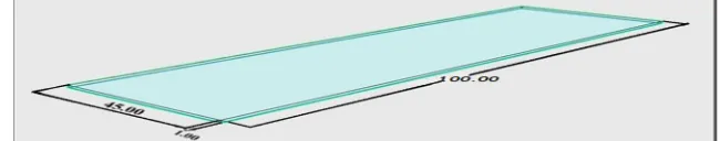
The work includes the Resistance Spot Welding of SS 316 stainless steel using Response surface methodology. SS316 stainless steel was taken for Resistance spot welding in the form of rectangular sheet and had the following dimensions:Length = 100mm, Width = 45mm, Thickness = 1mm.

Composition of SS316 is shown in table 1.Grade 316 is alloyed with molybdenum (~2–3%) for high-temperature strength, pitting and crevice corrosion resistance.

TABLE I

Chemical composition of 316 grade stainless steel

Element C Mn Si Ni Cr P S Mo Co Fe

% 0.06 0.55 0.31 9.17 17.37 0.03 0.008 2.25 0.128 71.20

B. Nugget Geometry Analysis

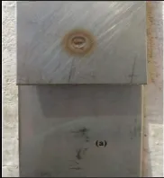
The specimen spot welded was used to determine the nugget width and HAZ width. The weld surface of the specimen was first polished with the use of polishing machine with emery grit paper size varying from 100 to 1000. Then etchant (Table 2) was used to analyze the image. Then nugget width and HAZ width was determined.

Figure 2 Visual inspection of nugget (Scale 1:1)

TABLE II

Stainless Steel Etchant (Carpenter 300 series)

Etchant Composition

Ferric Chloride 1.417 gm

Cupric Chloride 0.4 gm

Alcohol 20.33 ml

HCl 20.33 ml

Nitric Acid 1 ml

Further we used stereozoom under which we observed and measured the weld nugget and HAZ width as shown in fig. 3.

C. Tension Shear Test

For tension shear test BiSS nanoservo tensile testing machine was used. At first, the specimen was gripped in the jaw of the machine and then the grip was tightend. Then load was applied till specimen got fractured and data was recorded. Tension shear test is done to measure the strength of the joint under tensile loading. The specimen for tension shear test were lap welded as shown in fig 4.

Figure 4 Tension Shear test specimens

D. Microhardness Test

Vickers microhardness test is carried out to determine hardness of the joint. The specimen was held in the vice of the testing machine and a load of 500gm was applied on the specimen. The indenter was placed in a position where hardness is to be checked and then the output values of hardness were noted. For Vickers microhardness test, the welding was done as shown in fig. 5 and 6, and then all the welded specimens were cut along the XY

.

III. RESULTS AND DISCUSSION

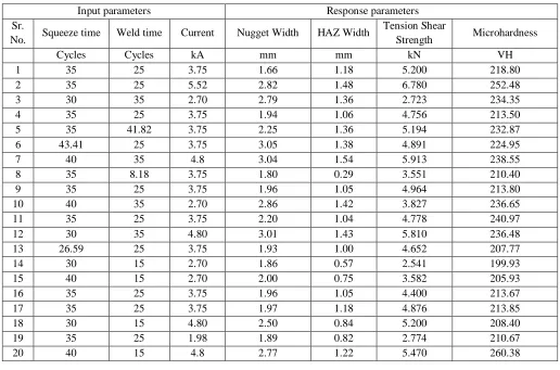
In proposed study, effect of process parameters (Squeeze time, Weld time and Current) on response parameters such as, Tension shear strength, microhardness, nugget width and HAZ width has been studied. Experiments were design using central composite design (20 runs). Response parameters values at different combination Spot welding input parameters are listed in table 3. During Welding higher tension shear strength, microhardness, nugget width and lower Nugget width are indications of better performance.Table 3 shows experimental results for tension shear strength, nugget width, HAZ width and microhardness.

Experimental results for Tension shear stength, nugget width, HAZ width and microhardness

A. Analysis of Nugget Width

Nugget width is a variable dependent on three factors-squeeze time, weld time and weld current.

TABLE IV Analysis of variance table for Nugget Width response

Factor Sum of Squares (SS) Degree of Freedom

(DF)

Mean Square

(MS) F-Value

P-Value Prob>F

Model 3.57 9 0.40 4.97 0.0098 Significant

A-Squeeze

time 0.40 1 0.40 4.98 0.0496

B-Weld

time 0.84 1 0.84 10.50 0.0089

C-Weld

current 0.80 1 0.80 10.05 0.0100

AB 7.813E-003 1 7.813E-003 0.098 0.7611

AC 1.125E-004 1 1.125E-004 1.406E-003 0.9708

BC 0.11 1 0.11 1.41 0.2625

A2 0.91 1 0.91 11.42 0.0070

Input parameters Response parameters Sr.

No. Squeeze time Weld time Current Nugget Width HAZ Width

Tension Shear

Strength Microhardness

Cycles Cycles kA mm mm kN VH

1 35 25 3.75 1.66 1.18 5.200 218.80

2 35 25 5.52 2.82 1.48 6.780 252.48

3 30 35 2.70 2.79 1.36 2.723 234.35

4 35 25 3.75 1.94 1.06 4.756 213.50

5 35 41.82 3.75 2.25 1.36 5.194 232.87

6 43.41 25 3.75 3.05 1.38 4.891 224.95

7 40 35 4.8 3.04 1.54 5.913 238.55

8 35 8.18 3.75 1.80 0.29 3.551 210.40

9 35 25 3.75 1.96 1.05 4.964 213.80

10 40 35 2.70 2.86 1.42 3.827 236.65

11 35 25 3.75 2.20 1.04 4.778 240.97

12 30 35 4.80 3.01 1.43 5.810 236.48

13 26.59 25 3.75 1.93 1.00 4.652 207.77

14 30 15 2.70 1.86 0.57 2.541 199.93

15 40 15 2.70 2.00 0.75 3.582 205.93

16 35 25 3.75 1.96 1.05 4.400 213.67

17 35 25 3.75 1.97 1.18 4.876 213.85

18 30 15 4.80 2.50 0.84 5.200 208.40

19 35 25 1.98 1.89 0.82 2.774 210.67

B2 _{0.11 1 0.11 1.37 0.2682}

C2 0.60 1 0.60 7.50 0.0209

Residual 0.80 10 0.080

Lack of Fit 0.65 5 0.13 4.43 0.0640 Not

significant

Pure Error 0.15 5 0.029

Cor Total 4.37 19

The Model F-value of 4.97 implies the model is significant. There is only a 0.98% chance that a "Model F-Value" this large could

occur due to noise.Values of "Prob > F" less than 0.0500 indicate model terms are significant. In this case A, B, C, A2, C2 are significant model terms.The "Lack of Fit F-value" of 4.43 implies there is a 6.40% chance that a "Lack of Fit F-value" this large could occur due to noise. Lack of fit is bad -- we want the model to fit. A negative "Pred R-Squared" implies that the overall mean is a better predictor of the response than the current model."Adeq Precision" measures the signal to noise ratio. A ratio greater than 4 is desirable. The ratio of 6.616 indicates an adequate signal. This model can be used to navigate the design space.

Nugget width of weld metal in coded form, Nugget width = 1.94 + 0.17 × A + 0.25 × B + 0.24 × C – 0.031 × A × B + 3.750E-003 ×A × C – 0.12 × B × C + 0.25 × A2 + 0.087 * B2 + 0.20 × C2

Nugget width of weld metal in actual form, Nugget width = 13.22764 - 0.65781 × Squeeze time + 0.045406 × Weld time – 0.89912 × Weld current – 6.25000E-004 × Squeeze time × Weld time +7.14286E-004 × Squeeze time × current -0.011310 × Weld time × Current + 0.010070 × Squeeze time2 + 8.73583E-004 × Weld time2– 0.18506 × Weld current2

The box plot (Figure 7) is a cubic view representing the eight desirable values for 23 full factorial experiments at the corners of the cube. Here maximum desirable nugget width is 3.11 mm at coordinates (A+:40, B+:35, C+:4.8).

Figure 7 Cube plot showing desirable values of nugget width

B. Analysis of HAZ Width

HAZ width is a variable dependent on three factors-squeeze time, weld time and weld current.

The Model F-value of 28.78 implies the model is significant. There is only a 0.01% chance that a "Model F-Value" this large could

is a 19.14% chance that a "Lack of Fit F-value" this large could occur due to noise. Non-significant lack of fit is good -- we want the model to fit.The "Pred R-Squared" of 0.7854 is in reasonable agreement with the "Adj R-Squared" of 0.9294."Adeq Precision" measures the signal to noise ratio. A ratio greater than 4 is desirable. The ratio of 19.816 indicates an adequate signal. This model can be used to navigate the design space.

HAZ width of weld metal in coded form = 1.09 + 0.10× A + 0.31 × B + 0.15 × C – 0.049 × A × B + 0.031 ×A × C – 0.069 × B × C + 0.053 × A2 – 0.076 * B2 + 0.039 × C2

HAZ width of weld metal in actual form = 1.01466 - 0.12593 × Squeeze time + 0.12730 × Weld time – 0.16583 × Weld current – 9.75000E-004 × Squeeze time × Weld time +5.95238E-003 × Squeeze time × current –6.54762E-003 × Weld time × Current + 2.11473E-003 × Squeeze time2 – 7.61786E-004 × Weld time2 + 0.035126 × Weld current2

TABLE V

Analysis of variance table for HAZ width response

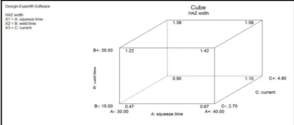
The box plot (Figure 8) is a cubic view representing the eight desirable values for 23 full factorial experiments at the corners of the cube. Here minimum desirable HAZ width is 0.470 mm at coordinates (A-:30, B-:15, C-:2.7).

Figure 8 Cube plot showing desirable values of HAZ width Factor Sum of Squares

(SS)

Degree of Freedom

(DF)

Mean Squares (MS)

F-Value P-Value

Model 1.94 9 0.22 28.78 <0.0001 Significant

A-Squeeze time

0.14 1 0.14 18.31 0.0016

B-Weld time 1.27 1 1.27 169.86 <0.0001

C-Weld current

0.30 1 0.30 40.66 <0.0001

AB 0.019 1 0.019 2.54 0.1423

AC 7.813E-003 1 7.813E-003 1.04 0.3313

BC 0.038 1 0.038 5.05 0.0485

A2 0.040 1 0.040 5.37 0.0429

B2 0.084 1 0.084 11.16 0.0075

C2 0.022 1 0.022 2.88 0.1203

Residual 0.075 10 7.494E-003

Lack Of Fit 0.052 5 0.010 2.30 0.1914 Non

significant Pure Error 0.023 5 4.547E-003

C. Analysis of Tension Shear Strength

Tension shear strength is a variable dependent on three factors-squeeze time, weld time and weld current.

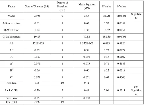
The Model F-value of 24.20 implies the model is significant. There is only a 0.01% chance that a "Model F-Value" this large could

occur due to noise.Values of "Prob > F" less than 0.0500 indicate model terms are significant. In this case A, B, C, B2 are significant model terms.The "Lack of Fit F-value" of 2.01 implies the Lack of Fit is not significant relative to the pure error. There is a 23.11% chance that a "Lack of Fit F-value" this large could occur due to noise. Non-significant lack of fit is good -- we want the model to fit. The "Pred R-Squared" of 0.7563 is in reasonable agreement with the "Adj R-Squared" of 0.9166."Adeq Precision" measures the signal to noise ratio. A ratio greater than 4 is desirable. The ratio of 17.733 indicates an adequate signal. This model can be used to navigate the design space.

Tensile shear strength of weld metal in coded factors = 4.84 + 0.21 × A + 0.31 × B + 1.21 × C – 0.013 × A × B – 0.22 ×A × C + 0.078 × B × C – 0.072 × A2 - 0.21 * B2 – 0.070 × C2

Tensile shear strength of weld metal in actual factors = -12.57104 + 0.40954 × Squeeze time + 0.11884 × Weld time + 2.91572 × Weld current – 2.60000E-004 × Squeeze time × Weld time – 0.042190 × Squeeze time × current + 7.45238E-003 × Weld time × Current – 2.88660E-003 × Squeeze time2 – 2.13233E-003 × Weld time2 – 0.063692 × Weld current2

TABLE VI

Analysis of variance table for tension shear strength response

The box plot (Figure 9) is a cubic view representing the eight desirable values for 23 full factorial experiments at the corners of the cube. Here maximum desirable tension shear strength is 6.050 kN at coordinates (A+:30, B+:35, C+:4.8).

Factor Sum of Squares (SS)

Degree of Freedom

(DF)

Mean Squares

(MS) F-Value P-Value

Model 22.94 9 2.55 24.20 <0.0001 Significa

nt

A-Squeeze time 0.62 1 0.62 5.93 0.0352

B-Weld time 1.32 1 1.32 12.52 0.0054

C-Weld current 19.83 1 19.83 188.30 <0.0001

AB 1.352E-003 1 1.352E-003 0.013 0.9120

AC 0.39 1 0.39 3.73 0.0824

BC 0.049 1 0.049 0.47 0.5107

A2 0.075 1 0.075 0.71 0.4183

B2 0.66 1 0.66 6.22 0.0318

C2 0.071 1 0.071 0.67 0.4306

Residual 1.05 10 0.11

Lack Of Fit 0.70 5 0.41 2.01 0.2311

Not Significa

nt

Pure Error 0.35 5 0.070

Figure 9 Cube plot showing desirable values of tension shear strength

D. Analysis of Microhardness

Microhardness is a variable dependent on three factors-squeeze time, weld time and weld current.

TABLE VII

Analysis of variance table for microhardness response

Factor Sum of Squares (SS)

Degree of Freedom (DF)

Mean Squares

(MS) F-Value

P-Value

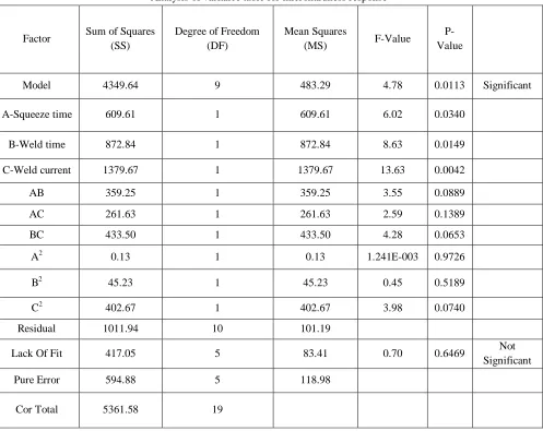
Model 4349.64 9 483.29 4.78 0.0113 Significant

A-Squeeze time 609.61 1 609.61 6.02 0.0340

B-Weld time 872.84 1 872.84 8.63 0.0149

C-Weld current 1379.67 1 1379.67 13.63 0.0042

AB 359.25 1 359.25 3.55 0.0889

AC 261.63 1 261.63 2.59 0.1389

BC 433.50 1 433.50 4.28 0.0653

A2 0.13 1 0.13 1.241E-003 0.9726

B2 45.23 1 45.23 0.45 0.5189

C2 402.67 1 402.67 3.98 0.0740

Residual 1011.94 10 101.19

Lack Of Fit 417.05 5 83.41 0.70 0.6469 Not

Significant

Pure Error 594.88 5 118.98

The Model F-value of 4.78 implies the model is significant. There is only a 1.13% chance that a "Model F-Value" this large could occur due to noise.Values of "Prob > F" less than 0.0500 indicate model terms are significant. In this case A, B, C are significant model terms. The "Lack of Fit F-value" of 0.70 implies the Lack of Fit is not significant relative to the pure error. The "Pred R-Squared" of 0.1716 is not as close to the "Adj R-R-Squared" of 0.6414 as one might normally expect. This may indicate a large block effect or a possible problem with your model and/or data. Things to consider are model reduction, response tranformation, outliers, etc."Adeq Precision" measures the signal to noise ratio. A ratio greater than 4 is desirable. Ther ratio of 8.659 indicates an adequate signal. This model can be used to navigate the design space.

Microhardness of nugget in coded factors = 218.96 + 6.68 × A + 7.99 × B + 10.05 × C – 6.70 × A × B + 5.72 ×A × C – 7.36 × B × C – 0.093 × A2 + 1.77 * B2 + 5.29 × C2

Microhardness of nugget in actual factors = 150.20768 + 0.86337 × Squeeze time + 7.23352 × Weld time – 46.98482 × Weld current – 0.13403 × Squeeze time × Weld time +1.08929 × Squeeze time × current - 0.70107 × Weld time × Current – 3.73346E-003 × Squeeze time2 + 0.017717 × Weld time2 + 4.79454 × Weld current2

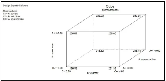
The box plot (Figure 10) is a cubic view representing the eight desirable values for 23 full factorial experiments at the corners of the

cube. Here maximum desirable microhardness is 248.15 VH at coordinates (A+:40, B+:15, C+:4.8).

Figure 10 Cube plot showing desirable values of microhardness

E. Optimization of Input Parameters

To achieve a optimum value for input parameters so that we get a better nugget width without expulsion of metal, lesser HAZ width and maximum tension shear strength, cross tension strength and microhardness we use desirability in Design Expert.

TABLE VIII Desirability table

Constraints Goal Lower limit Upper limit

Nugget width (mm) Maximize 1.66 3.05

HAZ width (mm) Minimize 0.29 1.54

Tension shear strength (kN) Maximize 2.541 6.78

Microhardness ( VH) Maximize 199.93 260.38

F. Solution

We get 21 solutions with varying desirability but the best suited and with maximum desirability percentage of 60.1 percent we use for further treatment. The optimized experimental value for maximum desirability can be seen in table 9.

TABLE IX Optimized result RUN NO SQUEEZE TIME (cycles) WELD TIME (cycles) WELD CURRENT (kA) NUGGET WIDTH (mm) HAZ WIDTH (mm TENSION SHEAR STRENGTH (kN) MICROHARD NESS (VH)

G. Confirmation Test

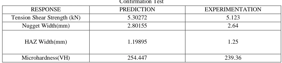
Confirmation tests were conducted so as to check whether the combination of optimal parameters produce the values of tension shear strength, nugget width,HAZ width and microhardness as nearby the value found out by the desirability test. The result along with the comparison is shown in table 10..

TABLE X Confirmation Test

RESPONSE PREDICTION EXPERIMENTATION

Tension Shear Strength (kN) 5.30272 5.123

Nugget Width(mm) 2.80155 2.64

HAZ Width(mm) 1.19895 1.25

Microhardness(VH) 254.447 239.36

Here, by comparing the predicted and experimental values, we can say that the experimental values of Tension Shear Strength, Nugget Width , HAZ width and microhardness differ from the predicted values by a little amount. Hence we can say that the predicted and experimental values almost agree with each other in terms of values.

A confirmation test is carried out to validate the analysis. Confirmation tests showed an error of 3.3% , 5.76% , 4.25% and 5.93% between the predicted and experimental values of tension shear strength , nugget Width , HAZ Width and microhardness respectively which was in acceptable range.

IV. CONCLUSION

Based on the achieved results following conclusions can be drawn :

A. All three independent parameters (current, Squeeze time and weld time) seem to be the influential parameters. The relationship between the input parameters and the response parameters has been developed. The predicted results appeared to be in good agreement with the measured ones.

B. It is found that with the increase in squeeze time, weld time and weld current all reponse parameters i.e. nugget width, HAZ width, microhardness and tensile shear strength increases.

C. From the mathematical model so developed, the input Current appears to be the most significant factor for all the response parameters (Tension shear strength, nugget width, HAZ width and microhardness).

D. Corresponding to highest desirability (maximum tension shear strength, nugget width, microhardness and minimum HAZ width), optimal combination of the input spot welding parameters appears to be Current = 4.8 kA, Weld time = 15 cycles, and Squeeze time = 40 cycles and the optimized value of nugget width, HAZ width, tension shear strength and microhardness are 2.80155 mm, 1.19895 mm, 5.30272 kN and 254.447 VH respectively.

E. A confirmation tests carried out to validate the predicted results display an error of 3.3% , 5.76% , 4.25% and 5.93% between the predicted and experimental values of tension shear strength , nugget Width , HAZ Width and microhardness respectively which is in acceptable range.

REFERENCES

[ 1 ] Parmar RS. Welding Engineering and Technology. Edition 2nd_{, editor. Khanna Publishers; 2010. Page 23-32}

[ 2 ] Parmar RS. Welding Processes and Technology. Edition 3rd, editor. Khanna Publishers; 2003. Page 328-356 [ 3 ] Montgomery D. Design and Analysis of Experiments. 2008

[ 4 ] Bilici M.K., Yukler A.I. and Kurtulmus M. (2011)’ The optimization of welding parameters for friction stir spot welding of high density polyethylene sheets’ , Materials and Design 32 4074–4079

[ 5 ] Kahraman N.and Bugra A.S. (2007)’ The influence of welding parameters on the joint strength of resistance spot-welded titanium sheets’, Materials and Design 28 420–427

[ 6 ] Bilici M.K., and Yukler A.I(2012)’ Effects of welding parameters on friction stir spot welding of high density polyethylene sheets’ Materials and Design 33 545–550

[ 8 ] Floreaa R.S, Bammanna D.J, Yeldella A., Solankic K.N. andHammia Y. (2013)’ Welding parameters influence on fatigue life and microstructure in

resistance spot welding of 6061-T6 aluminum alloy’ Materials and Design 45 456–465

[ 9 ] Shia H., Qiua R., Zhua J., Zhanga k., Yua H. and Dinga G. (2010) ’ Effects of welding parameters on the characteristics of magnesium alloy joint welded by resistance spot welding with cover plates’ Materials and Design 31 4853–4857

[ 1 0 ] Eisazadeha H., Hamedib M. and Halvaee A. (2010)’ New parametric study of nugget size in resistance spot welding process using finite element method’

Materials and Design 31 149–157