Interval cohort designs and bias in the estimation of per protocol effects: a simulation study

M E T H O D O L O G Y

Open Access

Interval-cohort designs and bias in the

estimation of per-protocol effects: a

simulation study

Jessica G. Young

, Rajet Vatsa

, Eleanor J. Murray

and Miguel A. Hernán

Abstract

Background: Randomized trials are considered the gold standard for making inferences about the causal effects of treatments. However, when protocol deviations occur, the baseline randomization of the trial is no longer sufficient to ensure unbiased estimation of the per-protocol effect: post-randomization, time-varying confounders must be sufficiently measured and adjusted for in the analysis. Given the historical emphasis on intention-to-treat effects in randomized trials, measurement of post-randomization confounders is typically infrequent. This may induce bias in estimates of the per-protocol effect, even using methods such as inverse probability weighting, which appropriately account for time-varying confounders affected by past treatment.

Methods/design: In order to concretely illustrate the potential magnitude of bias due to infrequent measurement of time-varying covariates, we simulated data from a very large trial with a survival outcome and time-varying

confounding affected by past treatment. We generated the data such that the true underlying per-protocol effect is null and under varying degrees of confounding (strong, moderate, weak). In the simulated data, we estimated per-protocol survival curves and associated contrasts using inverse probability weighting under monthly

measurement of the time-varying covariates (which constituted complete measurement in our simulation), yearly measurement, as well as 3- and 6-month intervals.

Results: Using inverse probability weighting, we were able to recover the true null under the complete

measurement scenario no matter the strength of confounding. Under yearly measurement intervals, the estimate of the per-protocol effect diverged from the null; inverse probability weighted estimates of the per-protocol 5-year risk ratio based on yearly measurement were 1.19, 1.12, and 1.03 under strong, moderate, and weak confounding, respectively. Bias decreased with measurement interval length. Under all scenarios, inverse probability weighted estimators were considerably less biased than a naive estimator that ignored time-varying confounding completely. Conclusions: Bias that arises from interval measurement designs highlights the need for planning in the design of randomized trials for collection of time-varying covariate data. This may come from more frequent in-person

measurement or external sources (e.g., electronic medical record data). Such planning will provide improved estimates of the per-protocol effect through the use of methods that appropriately adjust for time-varying confounders.

Keywords: Per-protocol effect, Inverse probability weighting, Interval cohorts, Simulation

*Correspondence:[email protected]

1_{Department of Population Medicine, Harvard Medical School & Harvard} Pilgrim Health Care Institute, Boston, USA

Full list of author information is available at the end of the article

Background

In randomized trials, the per-protocol effect is the effect that would have been estimated if all participants had adhered to their randomly assigned treatment strategies during the entire follow-up [1]. However, because adher-ence to the assigned treatment strategy is not in itself randomized, a naive comparison that excludes trial partic-ipants who fail to adhere to their assigned strategies will generally be biased [2].

For example, in a trial of a new treatment versus stan-dard of care to treat coronary heart disease, adherers to the treatment may be individuals who also tend to take antihypertensive treatment. Thus, a lower rate of disease among adherers may simply reflect their higher uptake of antihypertensives rather than a benefit of the treat-ment under study. Therefore, analyses that attempt to estimate the per-protocol effect typically need to adjust for prognostic factors that, like antihypertensive use in our example, are also associated with adherence. That is, per-protocol analyses are observational analyses of the randomized trial data and therefore need to adjust for confounders.

In randomized trials of point interventions that are administered shortly after randomization (e.g., a one-dose vaccination, a one-time screening test), adherence to the assigned intervention is fully determined at baseline and therefore can only be affected by baseline factors. The implication is that per-protocol analyses of point interven-tions only need to adjust for baseline confounders. On the other hand, in randomized trials of treatment strategies that are sustained during the follow-up (e.g., treatment for coronary heart disease, antiretroviral treatment for HIV-positive patients), adherence to the treatment strategy must also be sustained during the follow-up. The implica-tion of this potentially time-varying adherence is that per-protocol analyses of sustained strategies need to adjust for time-varying confounders — time-varying prognostic factors that affect treatment decisions — as well as for baseline confounders — baseline prognostic factors that affect treatment decisions [3–6]. For example, in a ran-domized trial to estimate the effect of two antiretroviral therapies on mortality, an increased alcohol intake dur-ing the follow-up is a time-varydur-ing confounder because it affects both the risk of death and of non-adherence to the assigned treatment.

It follows that valid estimation of the per-protocol effect of sustained treatment strategies requires adequate data collection of treatment and confounders after ran-domization. Many randomized trials collect such post-randomization data, but most only do so at pre-specified intervals (e.g., every 12 months). Because non-adherence may occur at any time during the follow-up, the con-founders measured at the pre-specified times may not be sufficient or relevant to adjust for non-adherence that

took place at an unknown time between the pre-specified measurement times.

In this paper, we review the impact of interval mea-surement on the estimation of per-protocol effects in randomized trials [7]. We conduct a simulation study to illustrate the potential magnitude of bias, even using causal inference methods for longitudinal settings such as inverse probability (IP) weighting [8], which appropri-ately account for time-varying confounders affected by past treatment.

Methods

Simulation design

We simulated data from a hypothetical randomized trial to quantify the effect of a new drug treatment compared to the standard of care on 5-year mortality risk.

Each individual is assigned to either the new drug treat-ment(Z=1)or to standard of care(Z=0)and followed until death or the administrative end of the study (60 months post-randomization), whichever comes first. We assume the exact month of death is known, as is common when studies link their data with death registries. For sim-plicity and without loss of generality, no individual is lost to follow-up.

Define t = 0,. . ., 60 as an index of follow-up month witht =0 the month of randomization (baseline). LetYt be an indicator of death by monthtwithY0 ≡ 0 for all individuals (all participants are alive and therefore at risk of the outcome at baseline) andAtan indicator of whether the new drug treatment is taken in montht. An individual deviated from the protocol in the first monthtin which

At=Z. In our simulated study approximately 40% of indi-viduals in both arms deviated from the protocol at some point during the follow-up. Figure1shows the cumulative proportion of protocol deviations over the study period by treatment arm.

In randomized trials, treatmentAtwill typically depend on both baseline (e.g., sex, race, baseline age) and post-baseline (e.g., lab measurements, concomitant medica-tions) risk factors for the outcome (e.g., death). LetLt =

(L1t,L2t)be a vector of such risk factors in montht, with

L1ta lab measurement (continuous) andL2tthe use of a concomitant medication (binary).

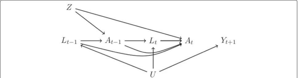
The causal diagram in Fig. 2 outlines the data-generating process of our simulated study. The node U

Fig. 1Proportion of participants who deviate from the protocol over the study period by treatment arm

We generated the data such that 100,000 individuals are assigned to each arm. We quantified bias for a given approach by the difference between the effect estimate obtained by that approach in this very large sample and the true effect value. Had we used a smaller sample size (e.g., 100 individuals assigned to each arm), random vari-ability could explain some differences between effect esti-mates and the true values of the effect (unless we had used the average over a large number of small samples, which is nearly equivalent to generating a single very large sample — this is illustrated in Additional file2).

We generated the data such that both the causal effect of treatmentAtfor alltand the direct effect of random-ization (Z) not mediated through treatment are null, as shown in Fig.2by the absence of anycausal paths(paths consisting of arrows going in the same direction) con-nectingZ, A_t−1, or At with the future outcome (Yt+1).

Therefore, both the intention-to-treat effect and the per-protocol effect are null.

Data-generating models

We generated longitudinal data according to the fol-lowing models for each subject i = 1,. . ., 200, 000 (i = 1,. . ., 100, 000 assigned Zi = 1 and i = 100, 001. . ., 200, 000 assignedZi = 0):Uiwas generated from a uniform distribution between 0 and 1. Then the following were generated for each month t = 0 until

t=59 or untilYt+1i =1 was generated, whichever came first:

• L1tiwas generated from a normal distribution such thatL1ti=6Ui−At−1i−cumavg(At−2i)+ 0.25cumavg(L1t−1i)+0.01t+iwith

i∼N(0,σ =2), cumavg(At−2i)is the cumulative

average of(A0i,. . .,At−2i), and cumavg(L1t−1i)is the cumulative average of(L10i,. . .,L1t−1i).

• L2tiwas generated from a Bernoulli distribution with meanpL2i, equal to the probability thatL2t=1given individuali ’s treatment and covariate history and survival tot, defined such that

logit(pL2i)= −5+3Ui+1.25cumavg(L1ti)+ 0.5L2t−1i+0.25At−1i+0.25cumavg(At−2i)+0.01t.

• For any individuali deviating from the protocol by

t−1(i.e.,At−1i=Zi), we setAti=At−1i(once an individual stops complying we assume they stay non-compliant). Alternatively, for any individuali complying with the protocol throught−1(i.e., all

Aji=Ziforj<t),Atiwas generated from a Bernoulli distribution with meanpAi, equal to the probability thatAt=1given individuali ’s treatment and covariate history and survival tot, such that

logit(pAi)=α0+0.4cumavg(L1ti)+0.35L2t−1i. (1) For individuals assignedZi=1(active treatment), we setα0=4.0. For individuals assignedZi =0

(standard of care), we setα0= −6.5.

• The death indicatorYt+1iwas generated from a Bernoulli distribution with meanpYi, equal to the probability thatYt+1=1given individuali ’s

treatment and covariate history and survival tot, such that

logit(pYi)=θ0+θ1Ui. (2)

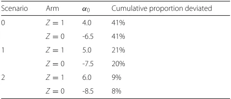
We considered three versions of this data-generating mechanism, varying the values ofθ0andθ1in the model (2). As we explain in the section“Defining and estimating the per-protocol effect”, given our data-generating models, the magnitude ofθ1determines the magnitude of time-varying confounding (andθ0the baseline event rate). We considered the following variations: “strong confounding” θ1 = 8 (θ0 = −11), “moderate confounding” θ1 = 3 (θ0 = −7), and “weak confounding”θ1 =0.5(θ0 = −6). We also considered three variations of the “strong con-founding” scenario under different choices ofα0in model (1) that reduced the chance of deviating from the protocol in both arms. Table1displays the cumulative proportion of protocol deviations by the end of the study period by treatment arm resulting from different choices ofα0.

R code implementing this simulation design is provided in Additional file1.

Defining and estimating the intention-to-treat effect We can define the intention-to-treat effect for any follow-up montht+1=1,. . ., 60 as a contrast of the cumulative risks in arm Z = 1, Pr [Y_t+1=1|Z=1] versus in arm

Z = 0, Pr [Yt+1=1|Z=0]. Our data generation, under

Table 1Proportion of protocol deviations under different choices ofα0in (1) by arm under “strong confounding” Scenario Arm α0 Cumulative proportion deviated

0 Z=1 4.0 41%

Z=0 -6.5 41%

1 Z=1 5.0 21%

Z=0 -7.5 20%

2 Z=1 6.0 9%

Z₌0 -8.5 8%

all scenarios, is consistent with no confounding for the effect of Z on survival, as illustrated in Fig. 2 by the absence of anyopen backdoor paths(open paths consist-ing of arrows goconsist-ing in different directions and, therefore, non-causal paths) [9] connecting the treatment arm indi-cator Z and the future outcomeYt+1. As a result, and because of the absence of loss to follow-up, a simple com-parison of the estimated risks (i.e., cumulative incidences) in armZ =1 versus armZ =0 is an unbiased estimator of the intention-to-treat effect Pr [Y_t+1=1|Z=1] ver-sus Pr [Y_t+1=1|Z=0] at any post-randomization time

t+1=1,. . ., 60.

We are able to recover the true intention-to-treat effect in our study, regardless of the presence of protocol devi-ations, because unbiased estimation of the intention-to-treat effect only relies on the random assignment ofZand no loss to follow-up. In contrast, unbiased estimation of theper-protocol effectrequires additional assumptions. Defining and estimating the per-protocol effect

Let Y_t+a=₁1 denote an individual’s indicator of death by montht+1, had she, possibly contrary to fact, continu-ously followed the protocol in arm Z = 1. Similarly, let

Y_t+a=₁0denote this outcome by montht+1, had she, instead, continuously followed the protocol in armZ=0. We can then formally define the per-protocol effect at montht+1 as a contrast of thecounterfactualrisks:

PrY_t+a=₁1=1|Z=1 versus PrY_t+a=₁0=1|Z=0. (3)

Note that, because Z was randomly assigned, we could alternatively define the per-protocol contrast as Pr

Y_t+a=₁1=1

versus Pr

Y_t+a=₁0=1

(unconditional on

treat-ment due to risk factors that affect both future adherence and survival. In Fig.2, such confounding is represented by open backdoor paths connectingAt−1andAttoYt+1, e.g., the pathAt ← Lt ← U → Yt+1. The data-generating models we have described previously ensure the pres-ence of this path by the dependpres-ence ofAton past values of the time-varying risk factors (L0,. . .,Lt), the depen-dence ofLtonU, and the dependence ofYt+1onU. As described in the section “Data-generating models”, we var-ied the degree of confounding (strong, moderate, or weak) by varying the magnitude of the parameterθ1in the model (2), which quantifies the strength of the dependence of

Yt+1onU.

Even though there is confounding for the per-protocol effect, the data generation mechanism in our study still allows unbiased estimation of the per-protocol effect as long as the study actually recorded all monthly covariates

Lt and treatmentsAt. Graphically, in Fig.2there are no open backdoor paths connectingAt−1andAttoYt+1

con-ditionalon past time-varying covariate changes [9]. For example, the open backdoor pathAt ← Lt ← U →

Yt+1is blocked by conditioning onLt. Note that the mea-surement of the variableU is unnecessary to adjust for confounding when the variablesLtare measured in allt.

However, valid estimation of the per-protocol effect (3) requires the use of adjustment methods that, like IP weighting, can handle the fact thatLt is affected by past treatment [3, 4, 10]. We give a detailed description of the IP weighting algorithm in Additional file2and the R code in Additional file1. Briefly, this approach involves: (1) as in the naive analysis, censoring participants when they deviate from their assigned protocol; (2) estimating IP weights which, at each time, are either 0 for censored participants or the reciprocal of the cumulative product of the time-varying probabilities of adherence to the pro-tocol given the participant’s measured confounder history up to that time for uncensored participants; and (3) esti-mating IP weighted survival curves. Risk differences and risk ratios can then be estimated by the complement of the IP weighted survival estimates. In addition to full mea-surement of the time-varying covariates, the validity of this approach also relies on correct specification of the model for the adherence probabilities in step 2.

Estimating the per-protocol effect under interval measurement

In practice, many randomized trials are conducted as interval cohorts such that adherence and covariates are recorded only at regular, scheduled follow-up times. When there are gaps between measurement times, the full history of treatment and covariate changes over the follow-up will not be completely observed and, generally, there will be unmeasured confounding; that is, under our data-generating assumption represented by Fig. 2, open

backdoor paths will remain after conditioning on only the measured past. Also, the full history of treatment changes will be only partially observed. Under a non-null scenario, failure to measure interim treatment changes may pro-duce an additional source of unmeasured confounding for treatment effects even at measured times; e.g., in Fig.2, were there an arrow fromAt−1intoYt+1, then an unblock-able open backdoor path (by failure to measure At−1) connectingAtandYt+1would be present. Partial knowl-edge of treatment changes thus also requires some form of imputation to estimate the per-protocol effect which is defined by counterfactual intervention in all months, not only months in which measurements are taken. Any imputation method may rest on strong assumptions, for example, imputation under the assumption that treat-ment does not change during measuretreat-ment gaps or under missing at random (MAR) assumptions [11].

Suppose, without loss of generality, that the inter-val between measurements is constant throughout the follow-up, e.g.,mmonths. We computed an IP weighted estimator of the per-protocol effect (3) and corresponding estimates of the counterfactual survival curves had all par-ticipants continuously complied with the protocol in each treatment arm under an interval-cohort scenario with

m=12, that is, a scenario in which treatment and covari-ate changes are measured only at baseline and then every 12 months. In interim months, treatment and covariates were set to the last measured value and the contribution to the weight cumulative product set to 1 for all subjects at these times. In this scenario, there will be residual con-founding by failure to adjust for time-varying covariates at unmeasured times. At measured times, IP weights can only be based on the inverse probability that a subject con-tinues to adhere in monthsgiven her partially measured confounder history. This probability is unknown under our data-generating mechanism (because we generated eachAtfrom the full history). Thus, we would also expect some bias due to model misspecification under this sce-nario. Here we chose to model adherence based on the cumulative average of past measured values of the contin-uous time-varying covariate (based on only the baseline and every 12-month measurement) and the current value of the binary covariate (as the value from the previ-ous month, the true value needed, will not be measured in this case).

Results

Intention-to-treat effect estimates

Fig. 3Intention-to-treat survival estimates by treatment arm

Table1). As expected, there is no bias in these estimates of the intention-to-treat effect; the curves completely overlap, which is consistent with the fact that the true intention-to-treat effect is null in all monthst+1. Naive versus IP weighted per-protocol effect estimates under full measurement

As illustrated by the top panel of Fig. 4, in our study a “naive” unweighted estimator that ignores time-varying confounders fails to recover the true null per-protocol effect because the curves do not overlap. Rather the esti-mates of the per-protocol 5-year risk difference and risk ratio for standard versus new treatment are 0.11 and 1.77, respectively. The bottom panel of Fig.4shows IP weighted estimates of the per-protocol effect under full measure-ment of the time-varying covariates(m=0). As expected, the estimated survival curves completely overlap, consis-tent with the truth, which is null. Figure4depicts results only under strong confounding. As expected, survival esti-mates across treatment arms under the naive approach that ignores confounding become closer as the strength of confounding weakens, while IP weighted estimates of the survival curves completely overlap under all scenarios (weak and moderate results are not shown).

IP weighted per-protocol effect estimates under interval measurement

In the interval-measurement scenario, we are generally unable to recover the truth of no per-protocol effect. In our study, IP weighted per-protocol effect estimates

under m = 12 diverged from the null as the strength of confounding increased. Specifically, Fig. 5shows that differences in the survival curves increase with the strength of confounding, which results in 5-year risk dif-ference/risk ratio estimates of 0.034/1.19 under strong confounding, 0.028/1.12 under moderate confounding, and 0.01/1.03 under weak confounding in our large sample.

Figure6illustrates that, even under strong confounding, bias decreases with more frequent measurement; esti-mates of the 5-year risk difference get closer to the truth of zero with decreasingm. Specifically, the IP weighted estimates of the risk difference/risk ratio were 0.017/1.02 under m = 3, 0.029/1.04 underm = 6, and 0.034/1.19 underm=12.

Finally, Fig. 7 illustrates that, even under strong con-founding and long interval measurement(m = 12), bias diminishes with decreasing non-adherence. Specifically, when the proportion of deviators decreased from approx-imately 40% (Scenario 0 in Table 1) to 20% (Scenario 1 in Table 1), the IP weighted estimates of the risk differ-ence/risk ratio were closer to the null. Bias was negligible, with risk difference/ratio estimates of 0.004/1.005, when there were fewer than 10% deviators per arm (Scenario 2 in Table1).

Discussion

Fig. 4Naive versus IP weighted estimates under strong confounding but complete measurement of covariate history

IP weighting, which appropriately adjust for time-varying confounders. However, IP weighted estimates were less biased than estimates from a naive analysis that ignored time-varying confounding.

We considered the simple case of per-protocol effects defined by static treatment strategies (e.g., always take the new treatment versus always take the standard treat-ment), but our approach could also be applied to dynamic strategies under which treatment changes in response to pre-specified events (e.g., a drug toxicity) [12–14]. Also, we considered a simulation without censoring by loss to follow-up. Censoring may prevent unbiased estimation of both per-protocol and intention-to-treat effects with-out sufficient and appropriate adjustment for baseline and time-varying covariates [10,15].

The bias created by interval measurement in the esti-mation of time-varying treatment effects has been pre-viously highlighted in the computer science literature [16] and in epidemiological studies such as the Fram-ingham Heart Study and the Nurses’ Health Study [7,

17]. In practice, the interval length required to make the

Fig. 5IP weighted estimates of per-protocol survival under the

m₌12 interval-measurement scenario and different confounding scenarios

Fig. 6IP weighted estimates of per-protocol survival under strong confounding and decreasing values ofm

necessary. In addition to more frequent in-person follow-up, complementary data sources such as electronic health records and pill cap monitors can help capture these changes.

Conclusions

The bias that arises from interval measurement high-lights the need for randomized trials designed to collect

Fig. 7IP weighted estimates of per-protocol survival under strong confounding and decreasing proportion deviating

Additional files

Additional file 1:R code to implement the simulation and IP weighted estimation procedures. (R 23 kb)

Additional file 2:Technical details of the IP weighted estimation algorithm and comparison of bias calculation using a single large sample versus average of many small samples. (PDF 166 kb)

Abbreviations

IP: Inverse probability; MAR: Missing at random

Acknowledgements

The authors thank Adam Young for assistance with increasing the computational efficiency of the R code.

Authors’ contributions

MAH and JGY conceived the idea for the manuscript. JGY and MAH designed the simulation and analysis plan and wrote the manuscript. RV and JGY wrote the R code for the simulation and IP weighted estimation. EJM contributed to the simulation design. RV and EJM reviewed and commented on the manuscript. All authors read and approved the final manuscript.

Funding

This work was funded by Patient-Centered Outcomes Research Institute (PCORI) grant 208643-5098419 and National Institutes of Health (NIH) grant NIH R37 AI102634.

Availability of data and materials

Not applicable.

Ethics approval and consent to participate

Not applicable.

Consent for publication

Not applicable.

Competing interests

The authors declare that they have no competing interests.

Author details

1_{Department of Population Medicine, Harvard Medical School & Harvard} Pilgrim Health Care Institute, Boston, USA.2_{Pathways M.D. Program, Harvard} Medical School, Boston, USA.3_{Department of Epidemiology, Harvard T.H.} Chan School of Public Health, Boston, USA.4_{Department of Biostatistics,} Harvard T.H. Chan School of Public Health, Boston, USA.5_{Harvard-MIT Division} of Health Sciences and Technology, Boston, USA.6_{Department of}

Epidemiology, Boston University School of Public Health, Boston, USA.

Received: 6 January 2019 Accepted: 16 July 2019

References

1. Hernán MA, Robins JM. Per-protocol analyses of pragmatic trials. N Engl J Med. 2017;14:1391–8.

2. Hernán MA, Hernández-Díaz S. Beyond the intention-to-treat in comparative effectiveness research. Clin Trials. 2012;1:48–55.

3. Robins JM. A new approach to causal inference in mortality studies with a sustained exposure period: application to the healthy worker survivor effect. Math Model. 1986;7:1393–512.

4. Robins JM. Addendum to “A new approach to causal inference in mortality studies with a sustained exposure period: application to the healthy worker survivor effect”. Comput Math Appl. 1987;14:923–45. 5. Robins JM. Health service research methodology: a focus on AIDS. In:

Sechrest L, Freeman H, Mulley A, editors. Washington, DC: US Public Health Service, National Center for Health Services Research; 1989. p. 113–59.

6. Robins JM. Correction for non-compliance in equivalence trials. Stat Med. 1998;17:269–302.

7. Hernán MA, McAdams M, McGrath N, Lanoy E, Costagliola D. Observation plans in longitudinal studies with time-varying treatments. Stat Methods Med Res. 2009;18(1):27–52.

8. Robins JM, Finkelstein D. Correcting for non-compliance and dependent censoring in an AIDS clinical trial with inverse probability of censoring weighted (IPCW) log-rank tests. Biometrics. 2000;56(3):779–88. 9. Pearl J. Causal diagrams for empirical research. Biometrika. 1995;82:

669–710.

10. Toh S, Hernán MA. Causal inference from longitudinal studies with baseline randomization. Int J Biostat. 2008;4(1):22.

11. Little RJA, Rubin DB. Statistical analysis with missing data. New York: John Wiley & Sons; 2002.

12. Hernán MA, Lanoy E, Costagliola D, Robins JM. Comparison of dynamic treatment regimes via inverse probability weighting. Basic & Clin Pharmacol & Toxicol. 2006;98:237–42.

13. Orellana L, Rotnitzky A, Robins JM. Dynamic regime marginal structural mean models for estimation of optimal dynamic treatment regimes, Part I: Main content. Int J Biostat. 2010;6:Article 7.

14. Orellana L, Rotnitzky A, Robins JM. Dynamic regime marginal structural mean models for estimation of optimal dynamic treatment regimes, Part II: Proofs and additional results. Int J Biostat. 2010;6:Article 8.

15. Little RJ, D’Agostino R, Cohen ML, Dickersin K, Emerson SS, Farrar JT, Frangakis C, Hogan JW, Molenberghs G, Murphy SA, Neaton JD, Rotnitzky A, Scharfstein D, Shih WJ, Siegel JP, Stern H. The prevention and treatment of missing data in clinical trials. N Eng J Med. 2012;367(14): 1355–60.

16. Schulam P, Saria S. Discretizing Logged Interaction data biases learning for decision-making; 2018. (pre-print)https://arxiv.org/abs/1810.03025. 17. Robins JM, Hernán MA, Siebert U. Effects of multiple interventions. In:

Ezzati M, Lopez AD, Rodgers A, Murray CJL, editors. Comparative quantification of health risks: global and regional burden of disease attributable to selected major risk factors. Geneva: World Health Organization; 2004. p. 2191–230.

Publisher’s Note