6 4 4m The Feed Enthalpy Computer 1963 pdf

THE FEED ENTHALPY COMPUTER

ABSTRACT: This study describes a generalized analog computer program for control of the feed stream enthalpy to a distillation column. It is based on the solution of a steady state heat balance equation written for the feed system to the column. Control is accomplished by feeding the solution

from the computer to a conventional recording-controlling instrument which automatically manipulates a control valve in the stream line to a feed preheater.

The program developed is designed for solution with an EAI PC-12 Process Control Computer. The programming flexibility of this computer

permits the use of standard, solid-state computing components. Scaling of the circuit is completely general, enabling the program to be utilized for a variety of columns having different operating conditions.

GENERAL

The importance of good regulation and control of

the three major heat inputs to distillation columns

in achieving improved operations is cited in the literature (1,2). Among the reasons presented

therein are:

(1) the difficulty of separation in many columns

(2) the Change in the dynamic character of columns

(3) the interaction of variables internal to the column, or external due to column auxili-aries

(4) the non-linear nature of significant

varia-·bles in a column

(5) the Change in demand upon column

oper-ation due to its dependency upon other parts of the process.

Even though control of distillation columns is a

well established art, and is adequately

docu-mented (3,4), there are certain heat input dis-turbances which require more than conventional

instrumentation for their control. One such dis

-turbance is the Change in enthalpy-heat conte

nt-of feed entering the column.

COMPUTER CONTROL OF FEED ENTHALPY Although the heat supplied to a column by the

feed is usually small in comparison to the total heat required for the separation, the importance to good column control of its being stabilized

should not be overlooked. It is generally desirable

Printed in U.S.A. 103

that the feed enthalpy be controlled at a level

which will result in the least operating costs while producing on-specification products. Re-gardless of whether the feed must enter at its bubble point temperature, partially vaporized, or subcooled, the problem of regulating it at a selected value becomes important to good column control.

One practical and economical method for regu -lating the feed heat content involves a special

purpose analog computer, called a Feed Enthalpy Computer. This approach has been found, by

simulation studies and extensive plant tests (1), to give excellent results where the feed enters at its bubble point temperature, partially

vaporized.

BOTTOM PRODUCT

---·HS ---TO ------CPF '--_-r------cpe

·

·

·

•

!

_,

,J, / ,

/"

:

FEED T, I

,

·

,

:

: I FEED STREAM

DISTILLATION

COLUMN

Figure 1. Feed Enthalpy Computer Control

of Distillation Column.

1 @) Electronic Associates, Inc. 1963

All Ri ghts Reserved

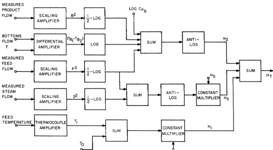
The concept of the Feed Enthalpy Computer is based on the inferential measurement of the total feed heat content by adding appropriate heat quantities; i.e., the initial heat content of the feed entering the economizer exchanger, the heat supplied to the feed by the economizer exchanger, and, the heat supplied by the steam feed pre-heater (refer to Figure 1). The computer con-tinuously calculates the feed heat content in BTU per pound of feed at the column input. Its output serves as the measured variable to an enthalpy recorder-controller whose output cas-cades into a steam flow controller that modulates the preheater steam flow to maintain a constant feed enthalpy. Inputs to the computer are pro-vided by conventional instrumentation in the form of signals from flow transmitters and thermo-couples.

Benefits which accrue from improved column control through regulation of the feed enthalpy by computer control are (1):

(1) Improved primary control of the separation (2) Lower operating costs

(3) Higher column throughputs (4) Smoother terminal stream flows

(5) A more predictable operation with less human attention.

DERIVING THE EQUATION

Control of the feed stream heat content is based upon the computer soluti.on of a steady state heat

CT MEASURED PRODU FLOW BOTTO FLOW T MS MEAS FEED FLOW URED URED MEAS STEAM FLOW FEED TEMP ERATURE SCALI NG AMPLIFIER DIFFERENTIAL AMPLIFIER SCALING AMPLIFIER SCALI NG AMPLIFIER THERMOCOUPLE AMPLIFIER

B2 _~-LOG 2

(TBI- TB2) LOG

F2 I

"2-LOG

L

S2

I -LOG 2

TI

SUM

TO

balance equation written for the column feed system. Referring to the schematic diagram of the feed portion of the distillation column (Figure 1) the total feed heat content per pound of feed, neglecting losses, is the sum of the following heat quantities.

H = c (T - T )

1 PF 1 0 Initial feed heat content above

some reference temperature To - BTU per pound of feed.

B

H_z= - _{c p (T} B - T )= The heat given up by the

F B I B2 b d

S

ottom pro uct stream to the feed in the economizer exchanger - BTU per pound of feed.

H = - H = The heat given up to the feed by the

3 F s

steam at the feed preheater - BTU per pound of feed.

The total heat content of the feed stream, per pound of feed, is then, in equation form;

or

ANALOG COMPUTER CIRCUIT

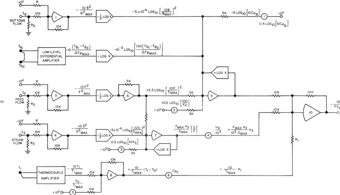
A suggested solution procedure outlining the mathematical operations required for solving equation 2 is shown in the information flow sheet of Figure 2. Using this diagram it is a relatively simple task to construct the computer circuit of Figure 3, Note that this circuit assumes that signals in the form of dc currents are available

LOG CPB

4

'--- SUM ANTI- H2

LOG

....

~

, -

SUM

r---~HS

....

HT

ANTI- CONSTANT

SUM

-LOG

I--

MULTIPLIER H3

CONSTANT HI

MULTIPLIEFi

1

CPF

[image:2.621.81.532.463.710.2]

-IOV

IS SOTTOMS

FLOW

-=

TSI

T82

-IOV

IF

~ _FLOW FEED

--IOV

IS STEAM

FLOW

-=

TI RS

RS R

10K

R

10K

R

LOW-LEVEL DIFFERENTIAL

AMPLIFIER

10K

108 2

2

-S MAX

IOF 2

2

-F MAX

-4 [ lOS ] 2

-5 x 10 LOGIO -S-M-A-X 5K -5 LOGIO [IOCPS]

>---~~---~----~VV~----~~~~

I

~--_o

5K

[ 10F ]2

t2.5LOG10 FMAX _5K

[ IOOJ +0.5 LOGIO K2

+IOV~

5K

10K

9

10K

10K

10K

RS

10K lOTI

T

-THERMOCOUPLE IMAX 10K

+_10_. (TI-TO) + _ _ 10_ HI

TIMAX CPF TIMAX

>-~--~~---~6}---~~---~

AMPLIFIER

TO TIMAX

10K

+IOV 5

[image:3.803.43.741.73.472.2]

for representing the square of the three flow rates. Square root operations on these flow signals are performed automatically, being programmed into the computer circuits. Temperatures are assumed to be measured by thermocouples whose outputs may be fed directly to amplifiers internal to the computer. Although the computer output as shown in Figure 3 takes the form of a dc voltage which varies from 0 to -10 volts it is possible to arrange the amplifier input and output circuits such that a dc current acceptable by conventional instruments is obtained.

The circuit of Figure 3 employs the following types of standard PC-12 Computing Components. DUAL OPERATIONAL AMPLIFIER (Type 6.368). Provides two high gain, chopper stabilized, tran-sistorized operational amplifiers for the per-formance of linear and non-linear mathematical operations. Low drift, high accuracy, field-proven circuits are designed specifically for general purpose on-line computing applications. Compact, plug-in modules mount in vapor-tight industrial housings. Dsed in the computer circuit of Figure 3 for scaling of input signals and for summing operations. Four dual modules or a total of eight amplifiers are required.

LOW LEVEL DIFFERENTIAL AMPLIFIER (Type 6.422). A transistorized, low-level differential amplifier designed for amplification of low-level signals. Design features include AC input section for added stability, 0.01% gain accuracy, and input impedances greater than 10 megohms. Used in the computer circuit of Figure 3 to accept and amplify differential thermocouple inputs for measurement of the bottoms flow differential temperature. One required.

THERMOCOUPLE AMPLIFIER (Type 6.406). Transistorized, low-level amplifier designed for amplification of low level thermocouple signals. Has similar characteristics as Type 6.422 Low Level Differential Amplifier but is designed speci-fically for single-ended input signals. Used in the circuit to accept and amplify a thermocouple input for measurem(?nt of the input feed temper-ature. One required.

COEFFICIENT SETTING POTENTIOMETERS

(Type 12.779).Provides four 10-turn, wire wound, 2000 ohm potentiometers with calibrated dials for setting of equation constants, constant inputs, and bias voltages. Six potentiometers required, Used in the circuit for introduction of scaling constants and for setting values for To' Hs ' cPF' cPB ' 1/2 LOG X DIODE FUNCTION GENERATOR (Type 16.215). Solid-state dual fixed diode func-tion generator for generating logarithms, ex-ponential functions, etc. When used with Ampli-fier 6.368 one generator will accept a positive voltage and generate a straight-line approximation of the logarithmic curve. The other generator

accepts a negative voltage to perform the same function. Internal circuit components are sized to produce an output of 2.5 LoglO(10X) for an input of X to facilitate the combined operations of square root and multiplication with a single amplifier. Current output for an input of X is 5 x 1O-4Log10(10X). Used in the circuitforform-ing the log of the signals representcircuitforform-ing the square of the flows. Three negative input generators are required.

LOG X DIODE FUNCTION GENERATOR (Type 16.214). Similar to the 1/2 Log X Generator but with internal circuit components sized toproduce an output of 5.0 Log10(10X) when used with an operational amplifier. Current output for an input of X is 10- 3 Log10(10X). Used in the circuit to perform anti-log operations and to take the log of the signal representing the bottoms differential temperature. Two positive input and one negative input generators are required.

These components, together with appropriate am-plifier input and feedback reSistances, system power supplies and control modules, patching sys-tem, etc., are mounted in an industrial housing to form the Feed Enthalpy Computer.

COMPUTER CIRCUIT SCALING

A generalized scaling scheme has been devel-oped for the computer circuit used to solve the steady- state heat equation. All signals and circuit components are expressed in terms of the ex-pected maximum values of the input variables.

Thus, once the column operating conditions are known, the circuit components and the computed signals can be completely specified using the scaled computer variables shown on the circuit of Figure 3 and a design equation developed from the scaling procedure.

The Appendix presents a detailed development of the scaling.

EXAMPLE

Assume that the column operating conditions are given as follows:

= 250,000 pounds per hour

F max = 500,000 pounds per hour

Smax = 20,000 pounds per hour

T = 200°F

lmax

= 750 BTU per pound of steam

From equation 2, the maximum value of HT is calculated as 250,000

HT = 0.532 (200) + ----(0.424)(300) +

max _500,000

20,000

- - - (750) = 106.4 + 63.6 + 30 = 200.0 500,000

Through use of the design equation developed in the Appen-dix ....

Then

Fmax K2

~T

Bmax Bmax

or

In addition

~T

10

H 200

Tmax 20

10

H

Tmax

Bmax Bmax

K2 =

--==-....:::=

20 F max

(300)(250,000) = 7.5 (20)( 500,000)

and

103 S

K _ max

3 - 20 Fmax

(1000)(20,000) (20)(500,000)

Potentiometer Settings become . . . .

(0.5)(.6274) = 0.3137

(0.5)(1.1248)

0.5624

2.0

tt3 - 0.5 Log10(10 K3 ) = 0.5 Log10(20) =

(0.5)(1.301) = 0.625

tt4 - Hs/I000 = 750/1000 = 0.750

5

li5 - To/Tl .~ 75/200 ~ 0.375 max

tt6 - c ~ 0.532

PF

Shunt resistors Rs are calculated to have the value

R _s =

10 10

(20 - 4) 10-3

104 = 625 ohms 16

Biasing resistors R are calculated to have the value ..

lO 104

R = (10 000) = , ,

-Rs lB. ' (625)(4 x 10 -3)

mw

40,000 ohms

Scaling resistor R 1 has the value

(10)(20)

(10,000) = (10,000)

200

= 10,000 ohms

Amplifiers of interest have the following scaled com-puter variables as outputs . . .

ttl0

-KS 20

(500,000)(7.5)

H2 = + H2

(300)(250,000)

= +

-20

while potentiometers tt4 and tt6 have outputs

scaled as follows . . .

(2)(500,000)

tt4 - + - - - H = +

-3 (1000)(20,000)

tt6 _ + _10 _ _

T

Imax

T

o

TB

2

F

B

S

-NOMENCLATURE-temperature of feed before entering econ-omizer; of.

arbitrary reference temperature used to compute H_{T ;} of.

temperature of bottoms product entering economizer; of.

temperature of bottoms product leaving economizer; 0 F.

f"ed flow rate; lb/hour.

bottom product flow rate; lb/hour.

steam flow rate; lb/hour.

difference in enthalpy of steam entering preheater and condensate (assumed con-stant); BTU/lb of steam.

average specific heat of feed; BTU/lb -of.

c

PB

K 2,

R s

R

Rj

K 3, KS

average specific heat of bottom product; BTU/lb - of.

scaling can stan ts.

shunt resistors used to develop voltage from current inputs; ohms.

biasing resistors on input of flow scaling amplifier; ohms.

input resistor for HI input to amplifier #10; ohms.

current representing square of input flows; millamperes.

SUBSCRIPTS

max expected maximum value or range of variable.

REFERENCES

-1. Lupfer, D,E., and M.W. Oglesby, "Automatic Control of Distillation Column Heat Inputs", Industrial and Engineering Chemistry, Dec. 1961.

2_ Lupfer, D_E., and M. W. Oglesby, "Feed En-thalpy Computer Control of a Distillation

Col-~", Control Engineering, Feb, 1962. 3. Lupfer D.E., and D,E. Berger, "Computer

Control of Distillation Reflux", ISA Journal, Vol. 6, No.6, June 1959,

4. Williams, T.J.; Industrial and 1008-19, 1956.

-

APPENDIX-INPUT SCALING AMPLIFIERS. The components of the following circuit must be sized such that, for the range of currents between the minimum and maximum,

e _o = 0 for IB . _mIn

R 10K

-10 V o---....J\/\/\,...---.

10K

Rs

Summing currents at amplifier grid:

Solving for resistance R:

Therefore, when e _o 0 and IB

=

IB . _mln

The current summation equation then becomes

Rs IB

10K

so that when IB = I Bmax ' e ₀ = -lOY

or

7

R = lOOK e + R L

o s-:B

R = lOOK

R _s IB . _mln

_ -1:L

R IB .

R

s

lOOK

R s I

s mln

Bmax -R

10

s

IB _max - IB _min e

0

=0 +

-10K

eo is to be made to represent the square of a flow, say B2, so computer variable is defined as -e = -k B2

where k is an amplitude scale factor. But

so

The scaled computer variable thus becomes

o

2

k· B 10

max

B2 -e = 1 0

-o B2

max

The Thermocouple Amplifier and the Differential Amplifier are scaled in exactly the same manner so as to restrict their maximum output to 10 volts. The circuits are more complex, however. Refer to the appropriate Service Manual for the exact procedure.

SCALING OF AMPLIFIER OUTPUTS

Amplifier #6: Summing Currents at grid (See Figure 3)

-4

-5 x 10 _LogIO

Amplifier #7: Summing currents

-4 [ Ioos2

J

-5 x 10 LogIO S~ax + 2.5 L 5K ogIO

+ _{10-3 LogIO [10 eo]} = 0

-2.5 LogIO

[S~~

J

2 + 2.5 Log IO

[i::J

2 - 5 LogIO [IOK3J + 5 LogIO [IoeoJ = 0

r.

IOK3 F max (S\J -5 LogIO

l

Smax

FJ

eo =

_K--,;~:;-F--,m=ax= (~\

Amplifier #8: Summing currents

e

=

10 (T - T ) o T1 1 0

max Amplifier #9: Summing currents

-4 lOB 5 -3

2

[J

-5 x 10 _{Log10 [Bmax ] - 5K Log10 10 CPB - 10 Log10}

+

~~

_{Log10 [F:: ] 2} +

5~

_Log10

[~;J

+ 10- 3 Log10 [10eo

J

= 0

-5 Log,O

[i::] -

5 Log,O [10

"vB] -

5 Log,O ['00

~'~:~:B2)]

+ 5 _Log10

[i::J

+ 5 Log10

[~;

] + 5 Log10 [10eo

J

= 0

- 5 Log,O [

9::)

(10 CPB) (00

~:~~B2l~

+ 5 LoglO

((i::J

(i~:)]

+ _{5 Log10 [10eo}

J

=

0

Amplifier #10: Summing currents Fmax K2 H2

+ 6.TB B 10K +

max max

+

[ F K

max 2

J

H +

[F K]

max 3 6. TBmax Bmax 2 103 Smax

10 H [ 1 ]

T1 1 _10K5

max (10K) T1max

-e _o

In order to sum these signals, all scale factors must be equal, or

The equation then becomes

F K

max 2

6.TB _{max max} B

9

e o

Representing e as a computer variable, and restricting the amplifier output to a 10 volts maximum .••

o

k·H

or

Thus, the design equation becomes

T

max

k

10 10

10

10

1 10

=

K5

=

HT

AI"

ELECTRONIC ASSOCIATES, INC. Long Branch, New Jersey