AN ENHANCED RULE APPROACH FOR NETWORK INTRUSION DETECTION USING EFFICIENT DATA ADAPTED DECISION TREE ALGORITHM

(1)

ISSN: 1992-8645 www.jatit.org E-ISSN: 1817-3195

OPTIMAL PLACEMENT OF TCSC USING LINEAR

DECREASING INERTIA WEIGHT GRAVITATIONAL

SEARCH ALGORITHM

1,2 _{PURWOHARJONO,} 2_{MUHAMMAD ABDILLAH,}2_{ONTOSENO PENANGSANG,} 2_ADI

SOEPRIJANT0

1

Electrical Engineering Department, University of Tanjungpura, Pontianak, Indonesia

2

Electrical Engineering Department, Institut Teknologi Sepuluh Nopember, Surabaya, Indonesia

E-mail: [email protected], [email protected], [email protected],

2_{[email protected]}

ABSTRACT

This paper represents the improvement of the Gravitational Search Algorithm method (GSA) using Linear Decreasing Inertia Weight (LDIW) which is implemented to determine the optimal placement of TCSC locations and the best rating of the TCSC in the standard limit on the electric power transmission lines. TCSC is one of FACTS devices which can perform the compensation of the power system. GSA method is a new metaheuristic method inspired by Newton's laws of gravity and mass motion. LDIW-GSA is used to control the speed of the particles on the GSA, so as to improve the performance of the GSA method. The implementation of LDIW-GSA used the Java-Bali 500 kV power system. Before optimization, TCSC load flow results indicated that there was 297.607MW of active power losses and 2926.825 MVAR of reactive power losses. While the results of TCSC load flow was 279. 405 MW of active power losses and reactive power losses was 2082.203 MVAR after optimization using GSA standard. It was obtained 278.655 MW of active power losses and active power losses of 1768.374 MVAR with the use of LDIW-GSA. It was better to be used to minimize power losses in transmission line and also it can improve the value of the voltage in the range of 1 ± 0.95 compared to GSA standards prior to placement optimization of TCSC.

Keywords: Gravitational Search Algorithm (GSA), Linear Decreasing Inertia Weight (LDIW), FACTS device, Thyristor Controlled Series Capacitor (TCSC), (AHPS)

1. INTRODUCTION

The more increased business in the industrial sector has led to the more need for active and reactive power. Such increase in reactive power on transmission lines causes increased power loss component with which worsen the voltage conditions, as a result, it requires components to control and compensate simultaneously the power losses in electrical power systems, especially in the transmission line. Those currently being developed are the FACTS (Flexible Alternating Current Transmission System) devices. FACTS is a component of the transmission system of alternating current using a power electronic control of thyristor for switching control, compensating for voltage drop and increasing power transfer capability [1-2].

There are several types of FACTS devices including: SVC (Static Var Compensator), TCSC (Thyristor Controlled Series Capacitor), TCPST (Thyristor Controlled Phase Shifting Transformer),

STATCOM (Static Compensator), UPFC (Unified

Power Flow Controller), TCPS (Thyristor

Controlled Phase Shifter), SSSC (Static

Synchronous Series Compensator) and IPFC (Interline Power Flow Controller) and others [3-10].

Artificial intelligence method developed in this study was the Gravitational Search Algorithm (GSA) one that would be improved using the Linear Decreasing Inertia Weight (LDIW). This GSA method was first introduced by Rashedi in 2009. It is a metaheuristic method inspired by Newton's laws of gravity and motion of mass [11]. Metaheuristic is a method to find a solution that combines the interaction between local search procedures and higher strategies to create a process managed to be out of local optima points and perform a search in the solution space to find a global solution [12].

(2)

SVC placement [13], economic dispatch (ED) on the power system [14], the voltage settings on the Java-Bali 500 kV power system [15], and optimization of reactive power dispatch [16].

LDIW-GSA is done by regulating LDIW optimal value that can be used to control the speed of the particles on the GSA method, so as to improve the performance of GSA methods.

In this study, LDIW-GSA could be used to determine the most optimal location for TCSC placement and also the TCSC best rating in the standard limit on the transmission line of power system. Besides, optimization using TCSC was also used to obtain the minimal power losses in transmission lines and voltage values werein the range of 0.95 ± 1.05 per unit.

2. FACTS DEVICES

Power flow on interconnected systems meets the Kirchhoff’s law. Resistance of the transmission line is smaller than the reactance, so the conduction was close to zero. Active power P_ijis transmitted on a transmission line between bus i and j which can be written in the following ties:

ij ij

j i ij

X V V

P = × sinθ (1)

(

i i j ij

)

ij

ij V VV

X

Q = 1 2− cosθ (2)

Where:

i

V and V_j = Voltage on the bus i and j.

ij

X = Reactance of the line.

ij

θ

= Angle between V and _i V_j

(V is phases)

The voltage difference of V_iand V_jon the

transmission line in a normal operation state was very small, so is

θ

_ij. The active power depends on

the

θ

_ij, and reactive power Q depends on the _ij V_i

and V_j. While the reactance X_ijchange affects

both.

3. THYRISTOR CONTROLLED SERIES

CAPACITOR (TCSC)

TCSC is a type of FACTS devices first developed. It has several components similar to the TCR, namely, among others, an inductor connected

in series with the thyristor bipolar. A thyristor works by setting the firing angle, so it can obtain some variations of inductive reactance causing a rapid reactive power exchange between the TCSC and the system. To compensate for a system that requires a capacitive reactive power, TCSC is installed in parallel with a bank capacitor.

TCSC in principle was installed in series with the existing transmission line. Reactance of the transmission channel settings can be done by controlling the TCSC reactance, so that power flow can be increased in other word increasing capabilities of the transmission line.

Fig.1. Simplified circuit of TCSC one phase

From Figure 1, it shows that TCSC is a combination of TCR components with a capacitor. TCR consists of a couple of inductors connected in

series with the thyristor. So the X_eq function is the

result of the thyristor firingangle:

( )

_{( )}

C L

eq

B B

X

+ − =

α

α 1 (3)

Where:

( )

α =−_ω1 _1−2_πα −sin_π

( )

2α _

L

B_L (4)

C

B_C =

ω

(5)

(3)

In Figure 2, thyristor firing angle is 0_⁰ and 90_⁰. It

stays at a distance ∆αfrom the point of resonance.

In Figure 2, the maximum compensation limit of

TCSC (X_max) is determined by the firing angle

max

L

α

and the minimum compensation limit

(X_min) by the firing angle ofαC_min.

To prevent excessive compensation, the

compensation degree of TCSC allowed is in the range of 20% inductive and 70% capacitive, so it applies:

7 . 0

min =− TCSC

r (6)

2 . 0

max = TCSC

r (7)

Fig.3. Model of TCSC on Transmission Line

In Figure 3, it can be determined the relationship between TCSC rating and reactance in the transmission line:

TCSC line

ij X X

X = + (8)

line TCSC rtscX

X = (9)

Where:

line

X = transmission line reactance

TCSC

r = TCSC compensation rating

4. IMPLENTATION OF THE PROPOSED

METHOD TO THE SYSTEM

Abbreviation and acronyms should be defined the first time they appear in the text, even after they have already been defined in the abstract. Do not use abbreviations in the title unless they are unavoidable.

The method used to set reactive power compensation is improved GSA using LDIW. LDIW-GSA can search several possible solutions simultaneously and also require none of any prior knowledge or the specific nature of the objective function. In addition, it is able to get the best solution to find optimal solutions in complex problems. It started in a random generation of initial population and then selected and mutated to get the best population.

4.1.

Encoding

Goals of this coding are to find the optimal location of TCSC in the range of equations and inequalities. Therefore, the configuration of TCSC is encoded by three parameters: location, type and value (rf). Each individual is represented by the number of TCSC on the string n, where n is the number of TCSC devices that need to be analyzed in the power system, as shown in Figure 4.

Fig.4. Individual configuration of the TCSC

The first values of each string correspond with location information. The value is the number of transmission line is the location of TCSC. Each string has a value different location. In other words, it must be ensured that in a transmission line there is only one TCSC. The second value is the type of TCSC. The values are expressed on a value of 1 for TCSC and the value 0 for the condition without TCSC equipment. Specifically, if there is no necessary TCSC on the transmission line, a value of 0 will work. Final value of rf is the value of the identifier of each TCSC. This value varies between -1 and +1. Real value of each TCSC is then converted by type of TCSC. TCSC has a range between −0.7X_line and0.2X_line, where X_lineis the reactance of the transmission line where the TCSC is installed. Therefore, it is converted into a real degree of compensation rtcsc using the following equation:

25 . 0 45 . 0

csc=rf × −

rt (10)

4.2.

Population

Initial population is generated from the following parameters:

FACTS

n = Number of TCSC is located

Type

n = Types of TCSC

Location

n = Possible locations for TCSC

Ind

n = The number of individuals from

(4)

Fig.5. The Calculation Of All Population

First, as shown in Figure 5 created a group of TCSC resulting string. For each string, the first value is selected randomly from the possible

locationsn_lokasi. The second value, which is a type

of TCSC, obtained by taking a number at random between the equipment has been selected. Specifically, after optimization, if no TCSC is required for this transmission line, the second value will be set to zero. The third value of each string, containing the value of the TCPST equipment, was chosen at random between -1 and +1. The above operation was repeated as nind times to obtain the whole initial population.

4.3.

Calculate Fitness

After encoding, each individual in the population was evaluated using the objective function.

Optimization problem associated with the

placement of TCSC, the objective function of this problem is used as fitness function. Fitness function is the calculation used to compare the quality of different solutions.

After encoding, each individual in the population was evaluated using the objective function.

Optimization problem associated with the

placement of TCSC, the objective function of this problem is used as fitness function. For this purpose, the TCSC is placed on the transmission line to pay attention to the power flow and voltage constraints. Objective function is used as the limit of TCSC placement to prevent under voltage or overvoltage on each bus and is able to reduce losses in power transmission line in the system.

Objective function for optimizing the placement of TCSC is to minimize losses on the transmission

line. Objective functions for optimal configuration of TCSC are:

- Active power loss minimization

Minimization of active power loss (Ploss) in the transmission line:

(

)

( )

∑

= = + − = n j i k k ij j i j i k

loss g V V VV

P , 1 2 2 cos

2 θ

(11)

Where: n = the number of transmission line, gk=

conductance of k branch, V_i and V_j = the voltage

magnitude on bus i and bus j, θ_ij= voltage angle

difference between bus i and bus

j.

- Equality Constrain

Power flow equation constrains is as follows:

nb i B G V V P P n

j ij ij

ij ij j i Di

Gi 0, 1,2,K

sin cos 1 = =       + − −

∑

= θ θ (12) nb i B G V V Q Q n

j ij ij

ij ij j i Di

Gi 0, 1,2,K

cos sin 1 = =       + − −

_∑

=

θ

(13)

Where: nb = number of buses, P_G and Q_G =

active and reactive power from generators, P_D and

D

Q = active and reactive load from the generator,

ij

G and B_ij = joint conductance and susceptance

between bus i and bus j.

- Inequality Constrain

Load bus voltage constraints inequality ( Vi ):

(

)

   − − = i V VL 1 exp 05 . 1 95 . 0

µ

for V etc

V if

i i 1.05

95 .

0 ≤ ≤

(14) Inequality constraints of switchable reactive power

compensation (Q_ci):

nc i Q Q

Q_cimin≤ _ci ≤ _cimax, ∈ (15)

Inequality constraint of reactive power generator (Q_Gi):

ng i Q Q

Q_Gimin≤ _Gi ≤ _Gimax, ∈ (16)

Inequality constraints of transformers tap setting (T_i):

nt i T T

(5)

(S_li):

nl i S

S_li ≤ _limax, ∈ (18)

Where: nc , ng and nt = number of switchable

reactive power sources, generators and

transformers.

To evaluate the optimization objective function on the placement of TCSC, the best and worst fitness is calculated each iterating as follows:

) ( min ) ( ) , 1

( fit t

t

best _j

N j∈ K

= (19)

) ( max ) ( ) , 1

( fit t

t

worst j N j∈ K

= (20)

Where:

fit

_j

(t

)

= Fitness in the jth agent at t time,

( )

t

best and worst

( )

t = the best fitness of all agents (the minimum) and worst (the maximum) fitness of all agents.

4.4.

Calculate Of The Gravitational Constant

To update the G gravitational constant in accordance with population fitness of the best agents (minimum) and worst (maximum) using equation (19) and (20). The gravitational constant

G(t) on t time is calculated as follows.

      − = T t G t

G( ) ₀exp α (21)

Where:

G

₀= Initial value of the gravitational

constant chosen at random,

α

= Constant,

t

= The

number of iterations,

T

= Total number of

iterations

4.5.

Calculate Of Inertia Masses And Gravity

To calculate the value of inertial mass (M) for each agent, equation (22) and equation (23) are used ) ( ) ( ) ( ) ( ) ( t worst t best t worst t fit t mg_i i

− −

= (22)

Where: fit_i

( )

t = Fitness to the agent

i

at

t

time.

∑

= = _N j j i i t mg t mg t Mg 1 ) ( ) ( )

( (23)

Where: Mg_i(t)= Mass of the agent

i

at

t

time.

4.6.

Calculate Of The Total Force

In this step, the total force acting on the agent i

( )

F_id t is calculated as follows:

( )

∑

( )

≠ ∈ = i kbestj j d ij j d

i t rand F t

F (24)

Where: rand_j= Random number between the

intervals [0.1], kbest_{= the initial set of agent K}

with the best fitness value and the largest mass. Forces acting on the mass i

(

M_i

( )

t

)

from the masses j

(

M_j

( )

t

)

at specific t time according to the gravity theory described as follows

(

() ()

)

) ( ) ( ) ( ) ( )

( t t

t R t M t M t G

t

_x

F

di

d j ij j i d

ij + −

× =

ε (25)

Where:R_ij

( )

t = Euclidean distance between the

agent i and agent j

(

( ) ( )

)

2

,X t

t

Xi j _,

ε

= a smack

constant.

4.7.

Calculate Of The Acceleration

In this step, acceleration of

( )

a_id

( )

t from the agent i at t time in dth dimensions is calculated with the laws of gravity and the laws of motion as follows. ) ( ) ( ) ( t Mg t F t a d i d i d

i = (26)

4.8.

Calculate Of Ldiw

LDIW was used to control speed and to maintain balance in influencing the trade-offs between global and local exploration abilities during the searching process. Furthermore, it was also a reduction of velocity parameters to avoid particle stagnation in the local optimum. If the value of LDIW is too large, the system will always be exploring new areas, consequently, the ability to explore the local value reduces. As a result, it fails to find a solution and if the value of inertia weight is too small then it can be stuck in local optimum. LDIW equation: [17-18]

(

)

max min max max k w w k w

wk = − −

(27)

Where:

max

w = maximum value

min

w = minimum value

max

k = iteration maximum.

k = iteration

(6)

4.9.

Calculate Velocity

In this step, n the velocity

( )

v_id

( )

t of ith agent at

t time in dth dimension is calculated through the law

of gravity and the laws of motion and the LDIW

(

ω

t) as follows.

) ( ) ( )

1

(t v t a t

v_id + =

ω

t× _id + _id (28)

Where:

t

ω

= linear decreasing inertia weight [0.2 - 1.2].

4.10.

Calculate Velocity

In this step, n the velocity

( )

v_id

( )

t of ith agent at t

time in dth dimension is calculated through the law

of gravity and the laws of motion and the LDIW

(

ω

t) as follows.

) ( ) ( )

1

(t v t a t

v_id + =

ω

t× _id + _id (29)

Where:

t

ω

= linear decreasing inertia weight [0.2 - 1.2].

4.11.

Update Position Agent Updating

In this step the next position of ith agent in dth

dimension d

(

x_id

( )

t+1

)

is updated as follows.

) 1 ( ) ( ) 1

(t+ =x_id t +v_id t+ d

i

x (30)

4.12.

Repetition

In this step, the steps from 4.2 to 4.11 are repeated until the iterations reach the criterion. At the end of the iteration, the algorithm returns the value associated with the position of the agent on a particular dimension. This value is the global solution of optimization problems as well.

LDIW-GSA algorithm, used to determine the optimal placement of TCSC locations and ratings, are shown in Figure 6.

Fig.6. Flowchart LDIW-GSA using TCSC

5. RESULT AND ANALYSIS

5.1.

Data Of Java-Bali 500 Kv Power System

The Java-Bali 500 kV power system is an interconnection system that delivers the power to customers in various areas in Java and Bali. The power is supplied from the electrical power produced by various sources of hydroelectric plants (located at the power plant of Cirata and

No

Yes Start

Stop

Update velocity (v) for each agent Input data of generation, transmission line, data TCSC, etc

Perform load flow calculation (Newton Rapshon Method)

Evaluate the fitness for each agent

Update the G, best and worst of the population

Calculate (M) and (a) for each agent

Meeting end of criterion?

Return best solution Generate initial population

Calculate LDIW

(7)

[image:7.612.287.531.94.610.2]

Saguling), steam power plant (located on the plant of Suralaya, Tanjung Jati, Paiton) and steam gas power plants (consisted of Grati, Muaratawar and Gresik plants). Single line diagram of power system can be seen in Figure 7.

Fig.7. Single Line Diagram Of Java-Bali 500 Kv Power System

This study used MVA base of 1000 MVA and kV base of 500 kV as the base of the Java-Bali 500 kV power system.

Transmission line parameters used in this study using per unit. Data line system of Java-Bali 500 kV system before using ohm. Therefore, it must first be converted into units of per unit.

Table I

Data Load And Generation Interconnection System Java-Bali 500 Kv

Bus

No Bus Name Bus code

Generator Load MW MVAR MW MVAR 1 Suralaya Swing 3211.6 1074.1 219 67 2 Cilegon Load 0 0 333 179 3 Kembangan Load 0 0 202 39 4 Gandul Load 0 0 814 171 5 Cibinong Load 0 0 638 336 6 Cawang Load 0 0 720 217 7 Bekasi Load 0 0 1126 331 8 Muaratawar Generator 1760.0 645.0 0 0 9 Cibatu Load 0 0 1152 345 10 Cirata Generator 948.0 200.0 597 201 11 Saguling Generator 698.4 150.0 0 0 12 Bandung

Selatan Load 0 0 477 254 13 Mandiracan Load 0 0 293 65 14 Ungaran Load 0 0 193 118 15 Tanjung Jati Generator 1321.6 90.0 0 0 16 Surabaya

Barat Load 0 0 508 265

17 Gresik Generator 900.0 366.3 127 92 18 Depok Load 0 0 342 95 19 Tasikmalaya Load 0 0 133 33 20 Pedan Load 0 0 365 101 21 Kediri Load 0 0 498 124 22 Paiton Generator 3180.0 917.3 448 55 23 Grati Generator 398.6 100.0 180 132 24 Balaraja Load 0 0 732 287 25 Ngimbang Load 0 0 264 58

Table 2

Line Data Of Java-Bali 500 Kv Power Systems

No From Bus

To Bus

R p.u

X p.u

½ B p.u 1 1 2 0.000626496 0.007008768 0 2 1 24 0.003677677 0.035333317 0 3 2 5 0.013133324 0.146925792 0.003530571 4 3 4 0.001513179 0.016928308 0 5 4 18 0.000694176 0.006669298 0 6 5 7 0.004441880 0.042675400 0 7 5 8 0.006211600 0.059678000 0 8 5 11 0.004111380 0.045995040 0.004420973 9 6 7 0.001973648 0.018961840 0 10 6 8 0.005625600 0.054048000 0 11 8 9 0.002822059 0.027112954 0 12 9 10 0.002739960 0.026324191 0 13 10 11 0.001474728 0.014168458 0 14 11 12 0.001957800 0.021902400 0 15 12 13 0.006990980 0.067165900 0.006429135 16 13 14 0.013478000 0.129490000 0.012394812 17 14 15 0.013533920 0.151407360 0.003638261 18 14 16 0.015798560 0.151784800 0.003632219 19 14 20 0.009036120 0.086814600 0 20 16 17 0.001394680 0.013399400 0 21 16 23 0.003986382 0.044596656 0 22 18 5 0.000818994 0.007868488 0 23 18 19 0.014056000 0.157248000 0.015114437 24 19 20 0.015311000 0.171288000 0.016463941 25 20 21 0.010291000 0.115128000 0.011065927

5.2.

Experimental Result

- The Load flow results before optimization using TCSC

[image:7.612.95.294.154.533.2]

(8)

the analysis before optimization using TCSC is shown in Figure 8 and Figure 9.

0.8 0.85 0.9 0.95 1 1.05

1 2 3 4 5 6 7 8 9 10 11 12 13 14 15 16 17 18 19 20 21 22 23 24 25

V o lt age b u s ( p u )

[image:8.612.92.521.68.243.2]

Number of bus

Fig.8. Voltage Profile Before Optimization Using TCSC

In Figure 8, it shows that the voltage variation of the Java-Bali 500 kV power system is in the range of 0.874 to 1.020 per unit. The highest voltage occurs at bus 1 (Suralaya), which is 1.020 per unit and the lowest voltage is found on the bus 20 (Pedan). Figure 6 also shows that there are eight buses having a voltage outside the range of 0.95 ± 1.05 per unit, namely: bus 12 (South London) = 0.948 per unit, bus 13 (Mandiracan) = 0.911 per unit, bus 14 (Ungaran) = 0.907 per unit, bus 19 (Tasikmalaya) = 0.875 per unit, bus 20 (Pedan)= 0.874 per unit, bus 21 (Karachi) = 0.902 per unit, bus 24 (Balaraja) = 0.982 per unit and bus 25 (Ngimbang) = 0.946 per unit.

0 100 200 300 400 500 600 1 -2 1 -2 4 2

-5 ₃-4

4

-1

8

5

-7 ₅-8

5

-1

1

6

-7 ₆-8 ₈-9

9 -1 0 1 0 -1 1 1 1 -1 2 1 2 -1 3 1 3 -1 4 1 4 -1 5 1 4 -1 6 1 4 -2 0 1 6 -1 7 1 6 -2 3 1 8 -5 1 8 -1 9 1 9 -2 0 2 0 -2 1 2 1 -2 2 2 2 -2 3 2 4 -4 2 5 -1 4 2 5 -1 6 P o w e r lo s s

Number of line

Real power loss (MW) Reactive power loss (MVAR)

Fig.9. Power Losses On The Transmission Line Before The Optimization Using The TCSC

Figure 9 shows the result of active power loss in transmission lines obtained before optimization using TCSC is 297.607 MW and the reactive power loss of 2926.825 MVAR with power supply from an active power plant for 10658.607 MW and reactive power of 7338.924 MVAR. The largest active and reactive power losses occur in lines 13-14 for 60.593 MV and 561.663 MVAR. While the smallest active and reactive power losses occur in 3-4 lines of 0.069 MW and 0.775 MVAR.

- The load flow results after optimization of using TCSC placement

Parameters used were the standard GSA and LDIW-GSA to determine the optimal placement of TCSC locations and its rating on the system Java-Bali 500 kV as shown in Table 3.

Table 3: Parameter In The Gsa And Ldiw-Gsa

No Parameter Value

1 Number of population 100 2 Number of iterations 100 3 Number of bus 25 4 Number of lines 30

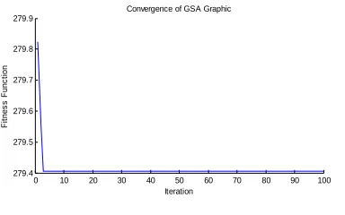
The results of the convergence curve after optimization using the TCSC from GSA standard and LDIW-GSA are shown in Figure 10 and Figure 11.

0 10 20 30 40 50 60 70 80 90 100 279.4 279.5 279.6 279.7 279.8 279.9

Convergence of GSA Graphic

[image:8.612.324.516.310.430.2]

Iteration F it n e s s F u n c ti o n

[image:8.612.93.302.438.562.2]

Fig.10. Convergence After Optimization Using TCSC Of GSA Standard

Figure 10 shows that the convergent

characteristics after optimization using TCSC from the standard GSA are able to produce more minimum values of the active power losses in transmission lines, when compared with the results before optimization using TCSC 279.405 MW and 2082.203 MVAR.

-0.8 -0.6 -0.4 -0.2 0 0.2 0.4 1-2 5-7 2-5 19-20 13-14 11-12 6-7 14-15 Rating (pu) L in e

[image:8.612.318.527.554.679.2]

(9)

In the Figure 11, it can be seen that the TCSC location and rating system in transmission system lines of Java-Bali 500 kV using standard GSA are the greatest on lines 1-2 at 0.1885 per unit and the smallest rating capacity occurs in lines 1112 at -0.0447 per unit.

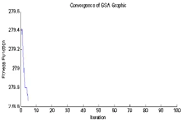
The results of the convergence curve after optimization using the TCSC from LDIW-GSA are shown in Figure 12 and Figure 13.

Fig.12. Convergence After Optimization Using The TCSC From LDIW-GSA

In Figure 12, it shows that the convergence characteristics after optimization using the TCSC from LDIW-GSA is able to produce more minimum values of the active power losses in transmission lines, when compared with load flow results before optimization using TCSC 278.655 MW and 1768.374 MVAR.

-0.7 -0.6 -0.5 -0.4 -0.3 -0.2 -0.1 0

11-12 18-19 13-14 16-23 4-18 19-20 25-14 14-16 24-4 14-15 6-8 5-11 14-20 21-22 6-7

Rating (pu)

L

in

[image:9.612.318.526.185.309.2]

e

Fig.13. Convergence After Optimization Using The TCSC From LDIW-GSA

Figure 13 shows that the location and rating of TCSC on and rating on transmission system lines of Java-Bali 500 kV using LDIW-GSA occur in channels 14-20 at -0.5804 per unit and occurs at the smallest rating for the channel 24-4 at -0.0723 per unit.

To keep the voltage at each bus in the range of 0.95 – 1.05 per unit, along with the smaller flowing power in each line than the maximum power,

compensation using the TCSC on the transmission line was carried out. The success of GSA standard and LDIW-GSA with the same parameter values is shown in Table 3 in completing optimization of the optimal location and rating placement using TCSC on Java-Bali 500 kV power system. It is shown in Figure 14 and Figure 15.

0.8 0.85 0.9 0.95 1 1.05

1 2 3 4 5 6 7 8 9 10 11 12 13 14 15 16 17 18 19 20 21 22 23 24 25

V

o

lt

a

g

e

(

p

u

)

Number of bus

[image:9.612.100.289.207.333.2]

Voltage (pu)-NR Voltage (pu)-GSA Voltage (pu)-IGSA

Fig.14. Comparison Of The Voltage Profile After Optimization Of TCSC Using The GSA, And

GSA-LDIW Before Optimization Of TCSC

Figure 14 shows that after optimization using TCSC, there is no more violation on voltage levels (0.95 ± 1.05 per unit), using either standard GSA or LDIW-GSA. This indicates that after optimization using the TCSC, the voltage profile on the electric power transmission line is getting better.

NR GSA IGSA

Real power loss 297.607 279.405 278.655 Reactive power loss 2926.825 2082.203 1768.374

0 500 1000 1500 2000 2500 3000 3500

[image:9.612.318.526.435.560.2]

Real power loss Reactive power loss

Fig.15. Comparison Of Power Line Losses After TCSC Optimization Using The GSA, GSA-LDIW And Before

Optimization TCSC

In the Figure 15 shows that after optimization using the TCSC, the power losses on transmission lines became minimal, whether using standard GSA and LDIW-GSA. The results of the power losses in

electrical power transmission lines after

[image:9.612.92.303.462.588.2]

(10)

6. CALCULATION

In this paper, the proposed LDIW-GSA was used for the placement of TCSC optimal location and rating on power system transmission line. The method used in this paper included methods of GSA standards and the improved one using the Linear Decreasing Inertia Weight (LDIW). Test results using Java-Bali 500 kV power system showed that the placement of the optimal location and the rating on TCSC using GSA standard and LDIW-GSA could improve the voltage value on the bus having a voltage drop to 0.95 ± 1.05 per unit and reduce the power losses in Java-Bali 500 kV electrical power system. Voltage improvement and power loss reduction in the Java-Bali 500 kV power system using LDIW-GSA is better than using the GSA standard and before optimization placement of TCSC.

ACKNOWLEDGEMENTS

The authors wish a highly gratitude to Indonesian Government especially The Directorate

General of High Education for graduate

Scholarship (BPPS) in which we receive along our study and the authors are very grateful to the Power System Simulation Laboratory, Department of Electrical Engineering, Sepuluh November Institute of Technology (ITS), Surabaya, Indonesia to all facilities provided during this research.

REFRENCES:

[1] Hadi Saadat, “Power System Analysis”,

Mc.Graw Hill Companies, Singapore, 2004.

[2] Imam Robandi, “Modern Power System

Design”, Andi, Yogyakarta, 2006 (Indonesian language).

[3] Umar, Adi Soeprijanto, Mauridhi Hery

Purnomo, “Placement Optimization of Multi Facts Devices In South Sulawesi Electrical System Using Genetic Algorithm”, National

Seminar on Information Technology

Applications, Yogyakarta, 2008, ISSN: 1907-5022 (Indonesian language).

[4] L.J. Cai, I. Erlich, “Optimal Choice and

Allocation of FACTS devices using Genetic Algorithms,” Proc. on Twelfth Intelligent

Systems Application to Power Systems

Conference”, pp. 1-6, 2003.

[5] Pisica, C. Bulac, L. Toma, M. Eremia,

“Optimal SVC Placement in Electric Power Systems Using a Genetic Algorithms Based

Method”, Paper accepted for presentation at 2009 IEEE Bucharest Power Tech Conference, June 28th - July 2nd, Bucharest, Romania.

[6] B. Bhattacharyya, B.S.K. Goswami, “Optimal

Placement of Facts Devices Genetic Algorithm for the Increased Load ability of a Power

System”, Warld Academy of Science,

Engineering and Technology, 2011.

[7] Rony Seto Wibowo, Naoto Yorino, Mehdi

Eghbal, Yosshifumi Zoka, Yutaka Sasaki,

“Facts Devices allocation With Control

Coordination Considering Congestion Relief and Voltage Stability”, IEEE Transactions on power systems, 2011.

[8] Siti Amely Jumaat, Ismail Musirin, Muhammad

Mutadha Othman,dan Hazlie Mokhlis,

“Optimal Location and Sizing of SVC Using Particle Swarm Optimization Technique”, First International Conference on Informatics and Computational Intelligence (ICI), Universitas Parahyangan, Bandung, 2011.

[9] Reza Sirjani dan Azah Mohamed, “Improved

Harmony Search Algorithm for Optimal

Placement and Sizing of Static Var

Compensators in Power Systems”, First International Conference on Informatics and Computational Intelligence (ICI), Universitas Parahyangan, Bandung, 2011.

[10] Kazemi, A. Parizad, H.R. Baghaee, “On the

[11] E. Rashedi, H. Nezamabadi-pour, S. Saryazdi,

“GSA: A gravitational search algorithm,” Information Sciences, 2009, vol. 179, pp. 2232-2248.

[12] Budi Santosa dan Paul Willy, “Metaheuristics

Method Concepts and Implementation”, Guna Widya Publishers, 2011, ISBN: 979545049-2 (Indonesian language).

[13] Esmat Rashedi , Hossien Nezamabadi-pour,

Saeid Saryazdi, Malihe M. Farsangi,

“Allocation of Static Var Compensator Usin Gravitational Search Algorithm”, First Joint Congress on Fuzzy and Intelligent Systems Ferdowsi University of Mashhad, Iran 29-31, 2007.

[14] S S. Duman, U. Güvenç, N. Yörükeren,

“Gravitational Search Algorithm for Economic

Dispatch with Valve-point Effects,”

(11)

[15] Purwoharjono, Ontoseno Penangsang,

Muhammad Abdillah dan Adi Soeprijanto,

“Voltage Control on Java-Bali 500kV

Electrical Power System for Reducing Power Losses Using Gravitational Search Algorithm”, International conference on informatics and computational intelligence (ICI), Universitas Parahyangan, Bandung, IEEE, 2011.

[16] Serhat Duman, Yusuf Sonmez, Ugur Guvenc,

dan Nuran Yorukeren, “Application of

Gravitational Search Algorithm for Optimal Reactive Power Dispatch Problem”, IEEE, 2011.

[17] J. C. Bansal, P. K. Singh, Mukesh Saraswat,

Abhishek Verma, Shimpi Singh Jadon, Ajith Abraham, “Inertia Weight Strategies in Particle Swarm Optimization”, Third World Congress

on Nature and Biologically Inspired

Computing, 2011, 978-1-4577-1123-7, IEEE.

[18] J. Xin, G. Chen, and Y. Hai., “A Particle