Munich Personal RePEc Archive
A selection analysis of returns to
education in China
Kang, Lili and Peng, Fei
April 2011
Online at
https://mpra.ub.uni-muenchen.de/44472/
1
RESEARCH ARTICLE
A Selection Analysis of Returns to Education in China
Lili Kanga,*, Fei Peng a
a
Centre for Research on the Economy and the Workplace (CREW), Business School, University of Birmingham, UK
*
Corresponding author: Birmingham Business School, University House, Edgbaston Park Road, Birmingham, B15 2TY, UK
Tel: +44 121 415 8446. Fax: +44 121 414 7380 E-mail address: [email protected] (L. Kang)
This paper estimates the economic returns to education in China from 1989
to 2009, using the China Health and Nutrition Survey (CHNS) dataset. We
find that education returns for one additional year generally increase from
2.6% in 1989 to 7.9% in 2009. Education returns, however, may reflect
signals of innate ability, or the accumulation of human capital. Moreover,
traditional Ordinary Least Square estimates may be biased by selection
problems and mix-ups of age group heterogeneity. Hence, we estimate the
marginal effects of schooling with the increasing labour markets experience,
using the Heckman Selection Model. We find that the education returns for
one additional year decline with labour markets experience, which support
human capital hypothesis for all age groups except the group educated
during the “Cultural Revolution”. Different dynamics of education returns in
the four age groups are identified with large influence of institutional
reforms in the labour markets, supporting the transition explanation of the
evolution of education returns in China.
JEL classification: J24, J31, P23, C52
2
Introduction
There is a well-established literature on the economic returns to education, since Schultz
(1961) and Mincer (1974). According to human capital theory, following Becker (1962),
education is an investment that produces knowledge acquisition and increases
productivity, which in turn leads to higher income. Human capital theory bears a strong
resemblance to vintage capital theory. The individual’s capital stock (his or her level of
education) can be treated as a factor of production in its own right and may gradually
depreciate with time (Byron and Manaloto 1990). Thus, the distribution of labour
incomes can be regarded as a function of education and experience, as in the benchmark
Mincerian model which involves regression of the natural logarithm of earnings against
educational attainment and working experience.
A large amount of empirical research, based on the Mincerian model, has been
carried out for many countries and time periods and confirms that better-educated
individuals earn higher wages, experience less unemployment, and work in more
prestigious occupations than their less-educated counterparts (Card 1999, O'Mahony
and Stevens 2009). Psacharopoulos and Patrinos (2004) finds that the education returns
for one additional year are 9.7% for world average, 9.9% for Asian average as well as
the 10.7-10.9% range for low and middle incomes. However, literature on economic
returns to education in China is still sparse and shows much lower rates of returns
compared with those from other countries, especially developing ones. An early study
on this topic for China was made by Byron and Manaloto (1990). Using a sample of
eight hundred adult workers from the city of Nanjing in 1986, they estimate a low rate
of returns between 1.2% and 3.7% for one additional year of schooling. Meng and Kidd
3
China Household Income Project (CHIP) 1988 data and finds a slightly larger but still
low rate of returns to education of 3.6% . Therefore, Fleisher et al. (2005) conclude that
China is an outlier, in that its rapid economic growth is associated with returns to
education remaining below the world average for comparable countries.
Low returns to education do not necessarily imply that education has no value in
China. It may be because the value of education has not been properly reflected as
private economic returns in labour markets. Fleisher and Wang (2004) find that the
wages of educated workers are well below their marginal product in China, and the
social returns to education will exceed the estimated private returns. Hence, the most
widely accepted explanation of lower Chinese education returns may be the explanation
of labour markets transition. Before 1978, wages of all workers were determined and
controlled through a rigid system in China, designed to reduce labour costs during the
rapid industrialization. Low wages were made possible by state-subsidized food prices
and state provision of non-wage benefits to workers and their families. Throughout the
economic reforms in China into the early 1990s, the wage differentials by levels of skill
and schooling still remained narrow. After the “socialist market economy” was
authorized in the early 1990s, the rigid wage system was gradually replaced by the
flexible wage system. 1 Thus, the wage reform in China freed up the compressed wage
differentials and thereafter had similar implications for the economic returns to
education.
The explanation of labour markets transition is supported by the literature dealing
with evidence of increasing returns to education over time, following the progress of
economic reforms. Recent research suggests that reform and marketization are finally
4
Wang 2005). Zhang et al. (2005) find a dramatic increase in education returns, from
only 4.0% in 1988 to 10.2% in 2001 for one additional year of schooling. Most of the
rise occurs after 1992 and supports the explanation of labour markets transition.
This paper provides alternative points of view on returns to education in China,
using recent available China Health and Nutrition Survey (CHNS) datasets from 1989
to 2009. We have three objectives. First, education has an important effect on wages but
it is not clear whether this is because education raises productivity or because education
is simply a signal of innate ability (Chevalier et al. 2004). We need to test whether the
returns to education in China reflect accumulation of human capital or are just signals of
innate ability. Following Qiu and Hudson (2010), we put the interaction of education
and experience into regressions for all employees and for four age groups. We calculate
the marginal effects of schooling at different percentiles of experience (Friedrich 1982,
Dreher and Gassebner 2007, Potrafke 2009) and then graph their trends with ranges of
standard errors. We find that Chinese data appear to strongly support the human capital
explanation.
Second, most studies on education returns in China only apply the traditional OLS
Mincerian model, which ignores the probable selection biases of employment. If the job
assignments in the labour markets are not random, OLS estimation of education returns
might be biased. The direction of biases is dependent on how jobs are assigned and how
people make self-selections in the labour markets (Roy 1951, Heckman 1974, Heckman
and Honoré 1990). Appleton et al. (2005) observe a continued influence of political
forces of loyalty, power, and patronage on the rewards for labour in the Chinese labour
markets. Considering the selection bias of employment, we compare the estimates of
5
Last, but not least, the aggregated estimates of repeated cross-section regressions
may be mix-ups of many heterogeneous cohorts and hence may suffer serious
composition biases (Solon et al. 1994). Li (2003) uses the 1988 CHIP data to classify
workers into three cohorts depending on when they started working: prior to economic
reform, up to 1979; in the early stage of urban reforms (1980 to 1987); or during the
advanced stage of urban reform (1988 to 1995). The average annual rates of returns to
college education were 7.7% for the pre-1979 cohort, 14.1% for the 1980–1987 cohort,
and 14.8% for the 1988–1995 cohort. Maurer-Fazio (1999) finds higher annual rates of
education returns for the young (under age 30, 6.6%) than for their elders (above age 50,
3.4%) in 1989. Fleisher and Wang (2005) estimate education returns in the first and
subsequent jobs, with workers grouped by the year of the first job, in order to observe
the impact of the “Cultural Revolution”. Their OLS estimators find that annual rates of
education returns to the younger cohorts (whose first jobs were in 1984, 1987 and 1990)
have received smaller returns to education than did the older cohorts (whose first jobs
occurred prior to 1970 and 1975, and were affected by the Cultural Revolution). These
cohort analyses reveal different views of education returns, compared to traditional
aggregated analysis. Hence, we estimate wage equations for four age groups which can
provide insights into the nature of labour markets changes and the fluctuations in returns
to schooling over time.
The rest of this paper is organized as follows: In section 2 we outline the
empirical specifications for our three objectives. In section 3 we describe our data and
present descriptive statistics. Estimates of the returns to schooling are presented in
6
Empirical specifications
Most previous literature relies on the theoretical foundations for returns to education,
laid down by Schultz (1961), Becker (1962) and Mincer (1974). We also estimate a
semi-logarithmic specification for the wages based on the Mincerian equation, given as:
) 1 ( Pr
ln 4 5 6 1
2 3 2
1
0
i i i i i i
i S Exp Exp Urban Gender
w
where the dependent variable lnwiis the log form of real hourly wage rate of employee
i. Wages consist of basic wages, subsidies and bonuses. We use the urban/rural
consumer price indices, classified by year and province from the China Statistics
Yearbooks, to deflate employees’ labour incomes. In the independent variables Si is
years of schooling; Expi is an employee’s potential labour markets experience,
measured as age minus years of schooling minus six (Katz and Murph 1992); Urbani is
a dummy variable for the urban areas; Genderi is a dummy variable capturing the wage
differential between men and women; and Pri is a set of province dummy variables.
Signal and human capital effects
There is debate whether the impact of education on earnings isolates the effects that are
caused by education from the consequences of innate ability. Economists have relied on
natural experiments, twins data, regression discontinuity, and field experiments to
control for innate ability and estimate the causal impact of education (human capital) on
earnings (see a review in Card (1999)). The CHNS cannot provide data for a direct
control on innate ability as do these classic models. However, we can develop Qiu and
7
accumulation of human capital. It is assumed that schooling (Si) that an individual
acquires is a function of innate ability (Ai ):
) 2 ( )
( i
i m A
S
Hence, more able individuals can grasp knowledge more rapidly and transform
schooling into human capital more efficiently, that is, Si/Ai 0. We can argue that
the basic theory underlying the earnings’ equation is that wages (wi) are a function of
human capital (Hi):
) 3 ( )
( i
i f H
w
In efficient labour markets, jobs with higher wages will be assigned to individuals
with higher productivity. Hence, individuals with higher human capital would have
higher wages, that is, f /Hi 0. Human capital of an individual itself is a function of
innate ability (Ai ), education-augmented human capital (Si) and experience-augmented
human capital (from on-the-job training or “learning by doing” processes,Expi) as
follows:
) 4 ( )
( )
( i i
i
i A h S g Exp
8
Human capital augmented by experience is also possibly influenced by innate
ability. More able individuals can grasp knowledge from on-the-job training or
“learning by doing” processes more rapidly and transform it into human capital more
efficiently, that is ( , ) 0
i i i A A Exp g
. However, an inverted U curve of experience in
earnings equations with quadratic experience is widely observed in the literature (for
China, see Appleton et al. (2005) and Qiu and Hudson (2010)). The individual’s capital
stock from experience can be treated as a factor of production in its own right and
gradually depreciates with time. Hence, we can firstly assume (for simplicity) that the
experience-augmented human capital is derived only from experience, and we also
assume linearity and that it is possible to separate the three types of human capital, in
equation (4). We cannot observe innate ability directly, hence we estimate wages as a
function of education and experience as:
) 5 ( )) ( ) ( ) (
( 1 i i i
i f m S h S g Exp
w
The total derivative of the wage function with respect to experience is as follows:
) 6 ( i i i i i dS S f dExp Exp f dw
We calculate the partial derivative of wage function with respect to schooling, and
allow the correlation between schooling and experience-augmented human capital. The
9 dS S S h S h Exp g H f dS S S h S S m H f dExp Exp f dw ( ) ) ( ) ( ) ) ( ) ( ( 1 (7)
For simplicity, we drop the individual subscript i. The first item is the quadratic
experience items in equation (1) to proxy the isolated experience effect on the wage.
The second item is the combination of signal and human capital effects of schooling on
the wage. The final item is the interaction of schooling and experience. If the only
impact of schooling is to proxy innate ability, schooling cannot enhance human capital,
that is, ( ) 0
S S h
. Then, the above equation becomes:
dA H f dExp Exp f dS S S m H f dExp Exp f dw
1( ) (8)
The coefficients of schooling are only capturing the effects of variations of innate
ability among individuals on wages. The impact of education on wages should be
constant over time, as the coefficients of experience and education interaction are zero.
Riley (1979) and Farber and Gibbons (1996) also argue that a basic condition for a
signalling equilibrium is that employers’ predictions based on education signals are
correct on average. If not, then education and experience could enhance productivity,
supporting the human capital theory.
Do the returns to schooling decline with rising experience since the individual left
formal education? Normally, with rising experience, education will depreciate. Hence,
10
show a negative correlation (substitution relationship) 0
) ( ) ( S h Exp g
and make the
coefficients of interaction items also negative because 0
H f
and ( ) 0
S S h
. But, in a
reforming society such as China, education chances may be very selective for innate
ability (for example, very strict college entrance examinations) or political virtue
(Broaded 1990). Individual human capital, enhanced by education and experience,
could be complementary if we consider the possibility that the innate ability or political
virtue also enhances human capital from experience. Education-augmented human
capital could be positively correlated with experience-augmented human capital. The
marginal effects of schooling may increase with experience in this simultaneous system.
We use pooled data to test the trend of education returns with rising experience over
time. Therefore, an interaction item is very important in our wage equation. After we
add the interaction variable of schooling and experience, and allow year dummies Y for
macro time dynamics, the empirical specification for our pooled data is as follows:
) 9 ( Pr ) * (
lnw0 1S 2Exp3Exp2 4 S Exp 5Urban6Gender7 8Y 1
Heckman selection bias
One important issue to consider is the fact that wages are only observed for individuals
actually working. Some individuals become inactive because they do not find a job, or
their reservation wages are higher than offer wages. There would be a potential
selection bias when estimating earnings equations. The Heckman selection model
provides a solution through an additional selection equation (Heckman 1976). People
11
attractive to employers and their opportunity cost of unemployment are higher.
Education increases expected wages over time, through higher wages when working
(the effect captured through the Mincerian equation above) and through a higher
probability of being employed (this effect will be captured through the Heckman
selection model below).
As derived from equation (9), the hourly wage rate is a function of schooling,
experience, urban, gender, province and year dummies, whereas the likelihood of
employment is a function of marital status and (implicitly) the wage (via the inclusion
of all above variables which determine the wage). The identifying variable for
employment selection is the marital status of a respondent, that is, a dummy variable
(0= single; 1=once married) which is widely used in literature (see an example for Italy,
in Brown and Sessions (1999)). Therefore, we assume that wage is observed if
0 Pr
) *
( 6 7 8 9 2
5 2 4 3
2 1
0
Married S Exp Exp S Exp Urban Gender Y
(10)
The inverse Mills ratio (lambda) defined as in (Heckman 1979) is designed to correct
for selectivity bias in the samples. A significant coefficient on the lambda term indicates
non-random selection into employment in the relevant sample.
Age groups
To gain more understanding of patterns of returns to schooling in China, we estimate
the regressions with separated age group samples. The four age groups are people born
12
choice of groups is based on the widely accepted structural break points in Chinese
modern history to allow heterogeneity of groups in our study. The first structural break
point is the foundation of the People’s Republic of China in 1949 and then two
structural break points based on the two baby boom periods (1950-1961 and 1962-1980).
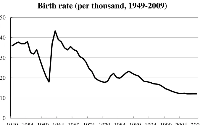
Finally, the full enforcement of the “One Child Policy” in 1981 defines the last group.
These structural break points can be clearly observed in a birth rate graph over the
period of 1949-2009 (see Figure 1). The birth rate was above 30 per thousand in the
1950s. The economic crisis from the “Great Leap Forward” and famine during the
period 1958-1961 resulted in 30 million extra deaths (Lin 1990), and the lowest birth
rate at 18.02 per thousand in 1961. Afterwards, with the economic recovery, China
experienced the largest baby boom, with the birth rate peaking at 43.37 per thousand in
1963. From 1961 to 1980, the newborns were about 310 million and comprised 23.5%
of the total population in 2009. 2 The large number of children born caused China’s
leaders to be very concerned about the growth potential of this extraordinarily large age
group. The “One Child Campaign” was launched in December 1979. In Feb 1980,
Guangdong province was the first province to make regulations for implementation,
followed by other provinces. The full enforcement of “One-Child policy” across country
started from 1981. There were two small peaks of the birth rate; between 1980 and 1982,
due to the implementation of China’s new Marriage Law in 1981; and the consequent
baby boom during 1984 and 1987. After that, the birth rate continued to decline to be as
low as 12.13 per thousand in 2009.
The special age group born 1950-1961 mainly received their education during the
“Cultural Revolution” period (1966-1976), when the leftist ideological goals of an
13
interrupted and replaced by continuous political movements (Qian and Smyth 2008).
They find this group has considerably lower returns to education than younger people
who received standardised education and entered the labour market during the urban
economic reform era.
(Figure 1 around here)
Data description
The data used in this paper are eight waves (1989, 1991, 1993, 1997, 2000, 2004, 2006
and 2009) of the CHNS dataset, which has been collected by the Carolina Population
Centre and the National Institute of Nutrition and Food Safety. The CHNS data cover
two decades of Chinese economic reform since 1989, and contain accurate information
on wages, education, and other demographic information which provides a basis for an
estimate of the returns to education. Eight provinces are covered by data in the period of
1989-1997 and nine provinces thereafter. 3 We exclude individuals working as farmers,
fishermen and hunters in the primary sector (mainly agriculture). Employees with a
salary (wage earners) between 16 and 65 years old are our basic sample. 4 The full
sample composed of employees, unemployed persons and self-employees is also
analyzed for the Heckman correction.
Table 1 represents the data description for the employee and full samples. For the
employee sample, the real hourly wage rate (based on 1995 RMB) is below 2 Yuan and
grows comparatively slowly before 1993. However, the hourly wage rate dramatically
doubles in the 4 years from 1993 to 1997, and then doubles again in the 9 years from
14
still grows by about 30%. The rapidly rising wage rate, especially after 1993, is also
observed by other authors, such as Yang et al. (2010).
The average schooling increases with rising wages by about 40% over the last two
decades (from 7.49 years in 1989 to 10.54 years in 2009). The working experience
decreases in the 1990s and increases in the 2000s, but still seems quite stable, ranging
between 20.15 years in 2000 to 24.33 years in 2009. About 60% of employees are males
and less than half the employees are in an urban area. About 80% of the employees are
married once, in our employee sample. The largest baby boom group, born in
1962-1980, occupies 37% of total employment in 1989, increasing to around 55% after 1993.
Hence, this group can benefit much more than others from the dramatic rising wages
after 1993. Actually, we find the special wage premium (or “rent”) in returns to
schooling of this group in the later analysis. The oldest group (born before 1950) keeps
on decreasing due to retirement. The youngest group (born in 1981 or after) has no
observation before 1997, and is still small in 1997, so we involve this group only after
1997. The share of the group born just after the foundation of China is stable at around
30% in the past two decades. Compared with the employee sample, the main difference
in the full sample is that the average years of schooling is lower (8.48 years in 1989 to
9.06 years in 2009). That is consistent with the findings that higher educated
individuals have higher probability to be employed (O'Mahony and Stevens 2009).
Table 2 shows descriptive statistics for the four groups in the pooled dataset of all
eight waves. For employees, the younger groups have higher real hourly wage rates and
years of schooling, but shorter potential labour markets experience. For example, the
youngest group (born in 1981 or after) has the highest hourly wage rate at 6.35 Yuan
15
the oldest), and lowest experience at 5.11 years (35.6 years less than the oldest). In
addition, the younger group has a higher female participation rate, higher participation
rates in rural regions and lower marriage rates.
Compared with employees, the full sample in the bottom panel has fewer years of
schooling than employees for all four groups, as we find in Table 1. Each group still has
distinguishable features as employees. These distinctive characteristics among groups
reflect volatile changes of Chinese society in recent decades, which imply
heterogeneous human capital accumulation of different groups from their education and
experience. If we only consider aggregated results, our estimate may be biased by the
composition shifts of groups.
(Table 1 around here)
(Table 2 around here)
Empirical results
Table 3 presents results of repeated cross-section OLS, as in equation (1). We find, in
common with others that education returns for one additional year generally increase
from 2.6% in 1989 to 7.9% in 2009. Results by groups are very similar to the
aggregated results in 1989, and this is consistent with the highly regulated wage setting
in the 1980s. With the ownership reform in the 1980s, the role of state-owned
enterprises has been weakened in the Chinese economy and has triggered the
transformation from a planned labour allocation system into a well-functioning labour
markets (Appleton et al. 2005). China authorized the “socialist market economy” to
16
reduction in rates of returns for the aggregated sample or groups in the early 1990s.
Camposa and Jolliffe’s (2003) study of Hungary, as well as that of Flabbi et al. (2008)
in examining eight transition economies (Bulgaria, Czech Republic, Hungary, Latvia,
Poland, Russia, Slovak Republic and Slovenia) argue that the skills acquired cannot be
easily transferred to a changed economic situation. Thus one would expect to see a
temporary decline to returns during any period of transition.
Between the trough of 1.4% in 1993 and peak of 9.4% in 2004, there is a
continuous rising trend of education returns for one additional year, which is also noted
in the most recent literature (for example, Liu et al. (2010)). After 1997, the four groups
experience different, but still increasing paths of education returns. Groups born before
1950 (8% for one additional year) and 1962-1980 (10% for one additional year) have a
peak in 2004 as for the employee sample, while the other two groups experience peaks
in 2006 (both around 10% for one additional year). The decline of education returns
after 2004 is caused mainly by the structural break of education returns of the group
born before 1950. Their dramatic fall of education returns (from the peak value to
insignificance) may reflect the human capital loss of compulsory retirement (especially
for women), and the rapidly depreciated human capital from education by the new
skill-biased technology (Liu et al. 2010). This loss can only be partly offset by the rising
employment proportions of the younger groups with still significant and high education
returns.
Table 4 shows the estimates from OLS regressions using the pooled dataset for all
eight waves. In order to test whether schooling only reflects the signal effects of innate
ability the interaction of schooling and experience has been regarded as an explanatory
17
one additional year. The highest coefficients are for groups born before 1950 and in
1981 or after (around 10%), but they are below 5% for the other two middle-aged
groups, suggesting lower rates of returns to schooling acquired during the Mao era. The
difference between Table 4 and Table 3 is derived from the interaction item of
schooling and experience. The coefficients of schooling in Table 4 are actually the
education returns when the labour market experience is equal to zero (Friedrich 1982).
Thus, the above results only show that the new entrants of the oldest and youngest
groups have higher education returns than new entrants in the other two groups. We
need to investigate the interaction item for the marginal effects of schooling with
experience.
The interaction variable of schooling and experience (divided by 100) is only
significantly negative for the full employee sample and the group born before 1950,
which casts doubt on the human capital explanation of education. In order to show the
dynamics of changing schooling returns by groups, we follow Dreher and Gassebner
(2007) and Potrafke (2009) to evaluate the marginal effects of schooling at various
points of the distribution of experience; namely at the 5th, 25th, median, 75th and 95th
percentiles of the interacted variable. 5 Using this method we can distinguish between
the impact of schooling on wage rates when the levels of experience are low and high.
All marginal effects are presented in the bottom panel of Table 4.
(Table 3 around here)
18
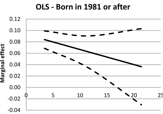
At the fifth percentile of potential labour markets experience (3.41 years), the
groups born before 1950 and in 1981 or after have the marginal effects of about 8.5% ,
higher than the other two middle-aged groups (each around 4.5% ), and similar to the
coefficients of schooling as experience equals 0. With increase in experience, the groups
born before 1950 and in 1981 or after have declining marginal effects of schooling.
However, the group born 1962-1980 has significant and increasing marginal effects,
which are also significant and stable over experience for the group born 1950-1961.
Figure 2 illustrates the trends of marginal effects of schooling with increasing
experience, with the lower and upper limits of one standard deviation for all the
employees and the four groups. Equation (7) shows that the coefficients of schooling
only reflect the signal of innate ability, because the coefficients of interaction are
insignificantly different from zero. Hence, the signal model fits the group born
1950-1961 in Table 4 and Figure 2 very well. If the interactions have negative coefficients,
the longer an individual has been out of school, the lower are his/her education returns
for one additional year of schooling, which fits the groups born before 1950 and in 1981
or after in Table 4 and Figure 2. Possible explanations for this difference include a
vintage effect, the rising quality of education, and greater mobility among younger
workers because they have made fewer employer-specific investments. People with
longer experience also are likely to be more constrained by wage compression and other
restrictions of past employment arrangements. Coefficients of schooling in this case
may include both signal and human capital effects of schooling, which would be a
traditional endogeneity problem. 6
Moreover, if the innate ability or education enhanced human capital can also
19
education enhanced human capital is positively correlated (hence complementary) with
experience enhanced human capital in equation (7). The longer an individual has been
out of school, the higher are his/her returns to education. Therefore, the group born
1962-1980 (if they are employed) can benefit from the “rent” from interaction between
education and experience. In this case, coefficients of schooling also include both signal
and human capital effects of schooling and show a rising trend in Figure 2.
(Figure 2 around here)
Next, we will use the Heckman selection model to correct selection biases. We
apply the Heckman selection model to provide consistent, asymptotically efficient
estimates for schooling. Table 5 presents the results of the Heckman selection model
using equation (9) and (10). The selectivity effect (lambda) is significant for the full
sample and the four groups. LR/Wald tests of independent equations (rho = 0) are easily
rejected for all ML specifications. These tests clearly justify the Heckman selection
model with data. By correcting the selection bias, the education returns for the full
sample decrease from 6% to 5.2% for one addition year, and decrease from 9.1% to 7.4%
for the group born before 1950. Returns do not change very much for the group born
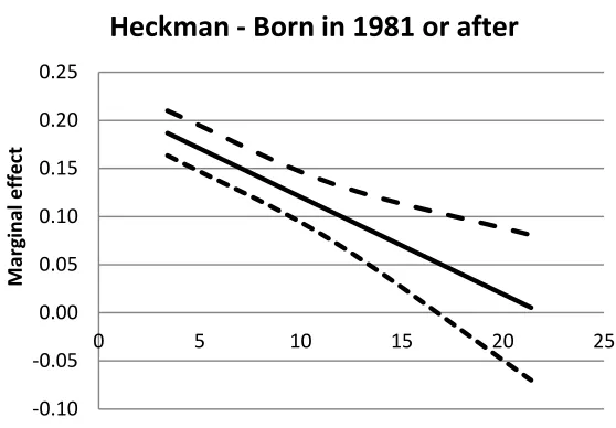
1950-1961, while the two younger groups have higher rates (from 4.1% to 11.8% for
the group 1962-1980; and from 9.3% to 22.1% for the group born in 1981 or after) than
in the OLS specification. Although these results are only point estimates, as experience
is equal to 0, we still find that they are closer to the results in other transition countries
20
The Heckman correction also has a significant effect on coefficients of interaction
of schooling and experience. Figure 3 illustrates all negative correlations (substitution
relationship) between marginal effects of schooling and experience. Compared with the
OLS estimates, the interactive variable of schooling and experience becomes
significantly negative for the largest baby-boom group (1962-1980) and the
one-child-policy group (in 1981 or after). Selection biases seem very serious for the group
1962-1980. The positive coefficients of interaction variable in OLS regressions just fit the
“rents”, as above-equilibrium wages in this group and could give rise to a “hitting the
jackpot” effect when a job is won (Peng and Siebert 2008). After we correct the
selection biases, the significantly positive trend of the group 1962-1980 in Figure 2 is
replaced by a significantly negative trend in Figure 3.
The only insignificant coefficient remains that to be found in the group born
1950-1961, the schooling years of which may only reflect the innate ability as we find
in the OLS regressions. This is not very surprising, because the group born 1950-1961
mainly received their education during the “Cultural Revolution” period (1966-1976),
when education chances were only allocated for selected students based on political
virtue. Those from families of workers, peasants or soldiers were deemed the most
“virtuous” and were among the first admitted. This has generated the label of
worker-peasant-soldier student (gong-nong-bing xueyuan) for those students entering college
during the early 1970s. Identification as a Cultural Revolution-era university student
continues to carry a negative loading and, in general, depressed opportunities for
advancement (Broaded 1990, Fleisher and Wang 2005).
For the only-child-policy group, even though the starting education for one
21
offsets the high coefficients of schooling as a new entrant. However, since we have only
a few hundred observations in the youngest group, any formal interpretation should be
concerned with caveats and needs further research. Therefore, the human capital
explanation of education is supported by our study, except for the group educated
during the “Cultural Revolution”.
(Table 5 around here)
(Figure 3 around here)
Conclusions
Schooling itself can be identified as an augmenting factor of human capital, or merely
as signals reflecting innate ability. Moreover, traditional aggregated Ordinary Least
Squares (OLS) estimates are biased by selection problem and mix-ups of group
heterogeneity. Hence, in this paper, we use the eight waves of the CHNS dataset to
estimate the rates of private returns to schooling in China over the last two decades. We
categorize data into four age groups according to the structural breaks of the birth rates
and estimate the marginal effects of schooling with increasing experience, using OLS
and the Heckman selection model.
The OLS estimates of education returns for all employees are 2.6% for one
addition year in 1989, then declining to around 1.5% in 1991 and 1993, possibly due to
the political campaigns and delayed reaction for labour market reforms. And then,
education returns increase to 9.4% for one addition year in 2004 before finally dropping
to 7.9% for one addition year in 2009 with the dramatic loss of human capital of the
22
years of the 1990s, but they experience heterogeneous dynamics later. This suggests a
substantial influence of institutional reforms in the labour markets. Our age group
analyses support the labour market transition explanation of the evolution of returns to
schooling over time.
The interactive variable of schooling and experience is used in the Heckman
model to test whether years of schooling only reflect the signal effects of innate ability.
We find that the education returns for one additional year decline with labour markets
experience, which supports the human capital hypothesis for all groups except the group
born 1950-1961, the schooling years of which may only reflect the innate ability or
political virtue as we find in the OLS regressions. This conclusion is not very surprising
because the group born 1950-1961 mainly received their education during the “Cultural
Revolution” period (1966-1976) when education chances were only allocated for
selected students based on political virtue. This group also has the lowest education
returns after we correct selection biases, just as found by Fleisher and Wang (2005).
Selection biases are very serious for the group born in the period 1962-1980. The
positive coefficients of interaction variable in OLS regressions just fit the “rents”
argument in this group with a “hitting the jackpot” effect when a job is won. After we
correct the selection biases, the significantly positive marginal effects of the group
1962-1980 in OLS are replaced by significantly negative marginal effects, as expected
by the human capital hypothesis. For the only-child-policy group, even though the
starting returns to schooling are as high as about 20%, the most rapid depreciation of
education offsets the high coefficients of schooling as a new entrant. However, since the
youngest group has many fewer observations than other groups in our sample, any
23
Acknowledgements
For useful comments we thank John Knight, Mary O’Mahony, Stan Siebert, Michela
Vecchi, Fiona Carmichael, Jim Love, Georgios Efthyvoulou and other participants of
the CEA conference (2010) at the University of Oxford and the workshop at the
University of Birmingham (2010). We thank Andy Briggs for his excellent editorial
assistance. The China Health and Nutrition Survey (CHNS) data are used with the
permission of the Carolina Population Centre based at the University of North Carolina
at Chapel Hill. Neither the original collectors of the data nor distributors bear any
responsibility for the analyses or interpretations presented here. All remaining errors are
our own.
Notes
1. The flexible wage system allows a variable component in the usual fixed wages.
The fixed wage includes the basic wages, seniority wage, insurance (medical,
unemployment and pensions) and a housing fund. The variable wage includes
bonuses, based on both individual productivity and enterprise profitability. The
system of allocated housing was largely abolished around 1998 and replaced
with a housing fund.
2. Data are from the Chinese Statistics Yearbook 2010.
3. 8 provinces (Liaoning, Jiangsu, Shandong, Henan, Hubei, Hunan, Guangxi and
Guizhou) for years 1989-1993; 8 provinces in 1997 (replacing Liaoning with
Heilongjiang); 9 provinces for years 2000-2009 (with both Liaoning and
24
4. The current retirement age in China is usually 60 for men and 50-55 for women.
But civil servants or professionals can postpone their retirement. Hence, we put
the upper limit as 65 for our sample.
5. We use the 5th percentile and 95th percentile to replace the minimum and
maximum experience years, which are extreme values and hence not
representative.
6. We acknowledge the possible endogeneity of schooling in the sense of
unobserved innate ability in the OLS regressions and the bias it can cause.
However, we would not correct the endogeneity biases in this paper because we
25
References
Appleton, S., Song, L. and Xia, Q., 2005. Has china crossed the river? The evolution of
wage structure in urban china during reform and retrenchment. Journal of
Comparative Economics, 33 (4), 644-663.
Becker, G.S., 1962. Investment in human capital: A theoretical analysis. The Journal of
Political Economy, 70 (5, Part 2: Investment in Human Beings), 9-49.
Broaded, M., 1990. The lost and found generation: Cohort succession in chinese higher
education. The Australian Journal of Chinese Affairs, 23, 77-95.
Brown, S. and Sessions, J.G., 1999. Education and employment status: A test of the
strong screening hypothesis in italy. Economics of Education Review, 18,
397-404.
Byron, R.P. and Manaloto, E.Q., 1990. Returns to education in china. Economic
Development and Cultural Change, 38 (4), 783-796.
Camposa, N.F. and Jolliffe, D., 2003. After, before and during: Returns to education in
hungary. Economic Systems, 27, 377-390.
Card, D., 1999. The causal effect of education on earnings. Handbook of Labor
Economics, Vol. 3A, Elsevier Science North-Holland, Amsterdam, New York
and Oxford, 1801-1863.
Chevalier, A., Harmon, C., Walker, I. and Zhu, Y., 2004. Does education raise
productivity, or just reflect it? The Economic Journal, 114 (499), F499-F517.
Dreher, A. and Gassebner, M., 2007. Greasing the wheels of entrepreneurship? The
impact of regulations and corruption on firm entry. CESifo Working Paper No
26
Farber, H. and Gibbons, R., 1996. Learning and wage dynamics. The Quarterly Journal
of Economics, 111, 1007-47.
Flabbi, L., Paternostro, S. and Tiongson, E., 2008. Returns to education in the economic
transition: A systematic assessment using comparable data. Economics of
Education Review, 27 (6), 724-740.
Fleisher, B., Sabirianova, K. and Wang, X., 2005. Returns to skills and the speed of
reforms: Evidence from central and eastern europe, china, and russia. Journal of
Comparative Economics, 33 (2), 351-370.
Fleisher, B. and Wang, X., 2005. Returns to schooling in china under planning and
reform. Journal of Comparative Economics, 33 (2), 265-277.
Fleisher, B.M. and Wang, X., 2004. Skill differentials, return to schooling, and market
segmentation in a transition economy: The case of mainland china. Journal of
Development Economics, 73 (1), 315-328.
Friedrich, R.J., 1982. In defense of multiplicative terms in multiple regression equations.
American Journal of Political Science, 26 (4), 797-833.
Heckman, J.J., 1974. Shadow prices, market wages, and labor supply. Econometrica, 42
(4), 679-694.
Heckman, J.J., 1976. The common structure of statistical models of truncation, sample
selection and limited dependent variables and a simple estimator for such
models. Annals of Economic and Social Measurement, 5, 475-492.
Heckman, J.J., 1979. Sample selection bias as a specification error. Econometrica, 47
(1), 153-161.
Heckman, J.J. and Honoré, B.E., 1990. The empirical content of the roy model.
27
Katz, L.F. and Murph, K.M., 1992. Changes in relative wages, 1963-1987: Supply and
demand factors. The Quarterly Journal of Economics, 107 (1), 35-78.
Li, H., 2003. Economic transition and returns to education in china. Economics of
Education Review, 22 (3), 317-328.
Lin, J.Y., 1990. Collectivization and china's agricultural crisis in 1959-1961. The
Journal of Political Economy, 98 (6), 1228-1252.
Liu, X., Park, A. and Zhao, Y., 2010. Explaining rising returns to education in urban
china in the 1990s. IZA DP No. 4872.
Liu, Z., 1998. Earnings, education, and economic reforms in urban china. Economic
Development and Cultural Change, 46 (4), 697-725.
Maurer-Fazio, M., 1999. Earnings and education in china's transition to a market
economy survey evidence from 1989 and 1992. China Economic Review, 10 (1),
17-40.
Meng, X. and Kidd, M.P., 1997. Labor market reform and the changing structure of
wage determination in china’s state sector during the 1980s. Journal of
Comparative Economics, 25, 403-421.
Mincer, J., 1974. Schooling, experience and earnings. National Bureau of Economic
Research, New York.
National Bureau of Statistics, D.O.C.S., 1999. Comprehensive statistical data and
materials on 50 years of new china. Beijing: China Statistics Press.
O'mahony, M. and Stevens, P., 2009. Output and productivity growth in the education
sector: Comparisons for the us and uk. Journal of Productivity Analysis, 31 (3),
177-194.
28
Potrafke, N., 2009. Did globalization restrict partisan politics? An empirical evaluation
of social expenditures in a panel of ) oecd countries. Public Choice, 140,
105-124.
Psacharopoulos, G. and Patrinos, H.A., 2004. Returns to investment in education: A
further update. Education Economics, 12 (2).
Qian, X. and Smyth, R., 2008. Private returns to investment in education: An empirical
study of urban china. Post-Communist Economies, 20 (4), 483-501.
Qiu, T. and Hudson, J., 2010. Private returns to education in urban china. Economic
Change and Restructuring, 43 (2), 131-150.
Riley, J., 1979. Testing the educational screening hypothesis. Journal of Political
Economy, 87, s227-52.
Roy, A.D., 1951. Some thoughts on the distribution of earnings. Oxford Economic
Papers, New Series, 3 (2), 135-146.
Schultz, T.W., 1961. Investment in human capital. American Economic Review, 51 (1),
1-17.
Solon, G., Barsky, R. and Parker, J.A., 1994. Measuring the cyclicality of real wages:
How important is composition bias? NBER working paper.
Yang, D.T., Chen, V.W. and Monarch, R., 2010. Rising wages: Has china lost its global
labor advantage? IZA DP No. 5008.
Zhang, J., Zhao, Y., Park, A. and Song, X., 2005. Economic returns to schooling in
29
[image:30.842.121.459.92.303.2]Source: National Bureau of Statistics (1999) ; China Statistics Yearbook 2010
Figure 1: Birth rate (per thousand, 1949-2009) 0
10 20 30 40 50
30 0.00 0.02 0.04 0.06 0.08
0 10 20 30 40 50
M ar g in al e ff e ct Experience
OLS - employee sample
0.00 0.02 0.04 0.06 0.08 0.10 0.12
0 10 20 30 40 50
M ar g in al e ff e ct Experience
OLS - Born before 1950
0.00 0.02 0.04 0.06 0.08 0.10
0 10 20 30 40 50
M ar g in al e ff e ct Experience
OLS - Born 1950-1961
0.00 0.02 0.04 0.06 0.08 0.10
0 10 20 30 40 50
M ar g in al e ff e ct Experience
31
Figure 2: Ordinary Least Square Model (OLS) - marginal effects and low/upper limits
-0.04 -0.02 0.00 0.02 0.04 0.06 0.08 0.10 0.12
0 5 10 15 20 25
M
ar
g
in
al
e
ff
e
ct
Experience
32 0.00 0.02 0.04 0.06 0.08
0 10 20 30 40 50
M ar g in al e ff e ct Experience
Heckman - Full sample
0.00 0.02 0.04 0.06 0.08 0.10
0 10 20 30 40 50
M ar g in al e ff e ct Experience
Heckman - Born before 1950
0.00 0.02 0.04 0.06 0.08 0.10
0 10 20 30 40 50
M ar gi n al e ffe ct Experience
Heckman - Born 1950-1961
0.04 0.06 0.08 0.10 0.12 0.14
0 10 20 30 40 50
M ar g in al e ff e ct Experience
33 Figure 3: Heckman Selection Model - marginal effects and low/upper limits
-0.10 -0.05 0.00 0.05 0.10 0.15 0.20 0.25
0 5 10 15 20 25
M
ar
g
in
al
e
ff
e
ct
Experience
34 Table 1: Data description for cross-sectional data
Employee sample (Ordinary Least Square model)
Variable All 1989 1991 1993 1997 2000 2004 2006 2009
Real hourly wage rate (Yuan) 3.93 1.22 1.46 1.73 3.49 5.13 6.07 6.93 9.05
Years of schooling (Years) 9.17 7.49 8.29 8.59 9.36 9.85 10.46 10.64 10.54
Experience (Years) 22.63 23.21 23.40 22.99 20.50 20.15 22.53 23.54 24.33
Male (%) 0.57 0.52 0.56 0.57 0.58 0.59 0.59 0.59 0.59
Urban (%) 0.48 0.49 0.51 0.48 0.48 0.44 0.50 0.47 0.47
Married (%) 0.79 0.75 0.80 0.77 0.74 0.74 0.87 0.88 0.88
Born before 1950 (%) 0.20 0.35 0.34 0.30 0.15 0.11 0.07 0.05 0.03
Born 1950-1961 (%) 0.29 0.28 0.31 0.30 0.29 0.29 0.30 0.30 0.25
Born 1962-1980 (%) 0.47 0.37 0.35 0.41 0.55 0.55 0.54 0.55 0.57
Born in 1981 or after (%) 0.04 0.00 0.06 0.09 0.10 0.16
Full sample (Heckman selection model)
Variable All 1989 1991 1993 1997 2000 2004 2006 2009
Years of schooling (Years) 8.48 7.16 7.90 8.12 8.37 8.95 8.79 9.04 9.06
Experience (Years) 24.77 23.45 22.28 22.42 22.36 22.14 26.82 27.87 28.80
Male (%) 0.51 0.51 0.53 0.54 0.52 0.52 0.49 0.49 0.48
Urban (%) 0.43 0.45 0.46 0.43 0.43 0.41 0.42 0.42 0.43
Married (%) 0.78 0.74 0.73 0.71 0.71 0.71 0.88 0.89 0.90
Born before 1950 (%) 0.23 0.35 0.32 0.29 0.24 0.19 0.18 0.16 0.11
Born 1950-1961 (%) 0.27 0.27 0.27 0.26 0.24 0.24 0.29 0.30 0.31
Born 1962-1980 (%) 0.43 0.38 0.41 0.45 0.50 0.45 0.41 0.41 0.43
Born in 1981 or after (%) 0.07 0.03 0.12 0.12 0.13 0.16
35 Table 2: Data description for pooled data (four age groups)
Employee sample (Ordinary Least Square model)
Variable
Born Born Born Born
before 1950 1950-1961 1962-1980 in 1981 or after
Real hourly wage rate (Yuan) 2.99 3.88 4.11 6.35
Years of schooling (Years) 6.53 9.41 10.06 10.89
Experience (Years) 40.71 26.31 13.57 5.11
Male (%) 0.63 0.6 0.53 0.5
Urban (%) 0.53 0.53 0.44 0.4
Married (%) 0.99 0.98 0.63 0.23
Full sample (Heckman selection model)
Variable
Born Born Born Born
before 1950 1950-1961 1962-1980 in 1981 or after
Years of schooling (Years) 5.88 8.43 9.6 10.36
Experience (Years) 44.09 30.21 14.39 3.83
Male (%) 0.5 0.51 0.51 0.52
Urban (%) 0.48 0.47 0.39 0.39
Married (%) 0.98 0.98 0.64 0.19
36 Table 3: Ordinary Least Square regressions
Employee sample All years 1989 1991 1993 1997 2000 2004 2006 2009
Years of schooling 0.043*** 0.026*** 0.015*** 0.014** 0.028*** 0.051*** 0.094*** 0.090*** 0.079***
0.003 0.004 0.004 0.006 0.007 0.008 0.009 0.007 0.007
R-squared 0.597 0.138 0.12 0.102 0.1 0.09 0.222 0.238 0.197
N 17,212 2,712 2,759 2,307 2,080 1,879 1,695 1,787 1,993
Born before 1950 All years 1989 1991 1993 1997 2000 2004 2006 2009
Years of schooling 0.026*** 0.028*** 0.009 0.014 0.02 0.070*** 0.080** 0.026 -0.106
0.004 0.006 0.006 0.009 0.019 0.016 0.033 0.043 0.068
R-squared 0.482 0.211 0.097 0.117 0.055 0.236 0.25 0.441 0.304
N 2,962 877 736 551 339 210 116 80 53
Born 1950-1961 All years 1989 1991 1993 1997 2000 2004 2006 2009
Years of schooling 0.048*** 0.026*** 0.020* 0.017 0.047*** 0.065*** 0.086*** 0.107*** 0.095***
0.005 0.009 0.011 0.012 0.013 0.016 0.017 0.015 0.018
R-squared 0.614 0.084 0.087 0.077 0.134 0.101 0.19 0.253 0.192
N 5,706 978 1,006 849 704 590 531 544 504
Born 1962-1980 All years 1989 1991 1993 1997 2000 2004 2006 2009
Years of schooling 0.051*** 0.026*** 0.014 0.014 0.022** 0.034*** 0.100*** 0.093*** 0.087***
0.004 0.009 0.009 0.012 0.009 0.01 0.012 0.01 0.008
R-squared 0.605 0.063 0.05 0.063 0.09 0.047 0.222 0.209 0.226
N 7,891 857 1,017 907 1,034 1,000 936 997 1,143
Born in 1981 or after Years in 2000s 1989 1991 1993 1997 2000 2004 2006 2009
Years of schooling 0.080*** 0.022 0.025 0.102*** 0.087***
0.013 0.154 0.038 0.023 0.016
R-squared 0.306 0.04 0.354 0.243 0.204
N 650 79 112 166 293
37 Table 4: Ordinary Least Square regressions
Employee
sample
Born before 1950
Born 1950-1961
Born 1962-1980
Born
in 1981 or after
Years of schooling 0.060*** 0.091*** 0.047*** 0.041*** 0.093***
0.005 0.019 0.013 0.008 0.026
School*experience/100 -0.067*** -0.178*** 0.004 0.063 -0.265
0.015 0.053 0.048 0.043 0.413
Experience 0.030*** 0.136*** 0.054*** 0.020** 0.032
0.003 0.023 0.014 0.008 0.076
Experience square -0.000*** -0.002*** -0.001*** -0.001*** 0.001
0 0 0 0 0.003
R-squared 0.598 0.484 0.614 0.605 0.308
N 17212 2962 5706 7891 653
Marginal effects of schooling (OLS)
Percentile 5% 25% 50% 75% 95%
Experience 3.41 11.57 21.39 31.83 47.98
Employee sample
Marginal effects 0.058*** 0.052*** 0.046*** 0.038*** 0.028***
standard error 0.004 0.003 0.003 0.003 0.004
Born before 1950
Marginal effects 0.085*** 0.071*** 0.053*** 0.035*** 0.006
standard error 0.018 0.014 0.009 0.004 0.007
Born 1950-1961
Marginal effects 0.047*** 0.048*** 0.048*** 0.049*** 0.049***
standard error 0.012 0.008 0.005 0.006 0.012
Born 1962-1980
Marginal effects 0.043*** 0.048*** 0.054*** 0.061*** 0.071***
standard error 0.006 0.004 0.005 0.008 0.015
Born
in 1981 or after
Marginal effects 0.084*** 0.062*** 0.036
standard error 0.015 0.028 0.067
38 Table 5: Heckman Selection Model
Full sample Born before 1950 Born 1950-1961 Born 1962-1980 Born
in 1981 or after
Ln (real hourly wage rate)
Years of schooling 0.052*** 0.074*** 0.049*** 0.118*** 0.221***
0.005 0.019 0.013 0.01 0.037
School*experience/100 -0.059*** -0.135*** -0.028 -0.105** -1.009**
0.015 0.052 0.046 0.052 0.499
Experience 0.027*** 0.117*** 0.062*** 0.116*** 0.369***
0.003 0.023 0.014 0.01 0.103
Experience square -0.000*** -0.001*** -0.001*** -0.003*** -0.014***
0 0 0 0 0.004
Select model
Married 0.080** 0.248* 0.234** -0.054 -0.220***
0.034 0.145 0.113 0.033 0.064
Years of schooling 0.210*** 0.246*** 0.282*** 0.182*** 0.217***
0.008 0.038 0.028 0.012 0.029
School*experience/100 -0.470*** -0.651*** -0.574*** -0.355*** -1.040***
0.022 0.09 0.083 0.06 0.398
Experience 0.172*** 0.062 0.193*** 0.213*** 0.535***
0.005 0.041 0.025 0.011 0.075
Experience square -0.003*** -0.001*** -0.003*** -0.005*** -0.022***
0 0 0 0 0.003
Mills (lambda) -0.04*** -0.06*** -0.04*** 0.67*** 0.80***
standard error 0.01 0.01 0.01 0.03 0.09
t value -5.04 -3.81 -3.27 20.68 8.87
Wald test of indep. Eqns. (rho=0)
25.62*** 13.51*** 10.79*** 342.22*** 70.59***
0 0.0002 0.001 0 0
N 40,933 9,494 11,668 17,218 2,553
Marginal effects of schooling (Heckman selection model)
Percentile 5% 25% 50% 75% 95%
Experience 3.41 11.57 21.39 31.83 47.98
Full sample
Marginal effects 0.050*** 0.045*** 0.039*** 0.033*** 0.024***
standard error 0.004 0.003 0.003 0.003 0.004
Born before 1950
Marginal effects 0.069*** 0.058*** 0.045*** 0.031*** 0.009
standard error 0.017 0.013 0.008 0.004 0.007
Born 1950-1961
Marginal effects 0.048*** 0.046*** 0.043*** 0.040*** 0.036***
standard error 0.012 0.008 0.005 0.006 0.011
Born 1962-1980
Marginal effects 0.114*** 0.106*** 0.096*** 0.085*** 0.068***
standard error 0.009 0.006 0.006 0.009 0.017
Born
in 1981 or after
Marginal effects 0.187*** 0.104*** 0.005
standard error 0.023 0.030 0.075