Munich Personal RePEc Archive
Do consumers prefer offers that are easy
to compare? An experimental
investigation.
Crosetto, Paolo and Gaudeul, Alexia
Max Planck Institute of Economics, Max Planck Institute of
Economics
20 September 2012
D
O CONSUMERS PREFER OFFERS THAT ARE EASY TO
COMPARE?
AN EXPERIMENTAL INVESTIGATION.
1Paolo Crosetto2 and Alexia Gaudeul3
September 20, 2012
1We wish to thank Nicolas Berkowitsch, Alena Otto and Robert Sugden for their comments and
suggestions. This paper was presented at the Max Planck Institute for Economics in Jena in April 2011, at the workshop for Experimental Methods and Economic Modeling in Capua in June 2011, at the Max Planck Institute for Human Development in Berlin in June 2011, at the International Confer-ence of the Economic SciConfer-ence Association in Chicago in July 2011, at the European ConferConfer-ence of the Economic Science Association in Luxembourg in September 2011, at the Department of Economics, Business and Statistics (DEAS) of the University of Milan in December 2011 and at the Conference of the European Economic Association in M´alaga in August 2012. The experiment’s interface and ran-domized menu generation were programmed with Python (van Rossum, 1995). Data analysis and regressions were performed with Stata (StataCorp, 2009). Simulations were run with Octave (Eaton, 2002).
2Strategic Interaction Group (ESI), Max Planck Institute for Economics, Jena. email:
crosetto@econ.mpg.de
3Strategic Interaction Group (ESI), Max Planck Institute for Economics, Jena. email:
Abstract
Firms can exploit consumers’ mistakes when facing complex purchasing decision problems
but Gaudeul and Sugden (2012) argue that if at least some consumers disregard offers that
are difficult to compare with others then firms will be forced into adopting common ways
to present their offers and thus make choice easier. We design an original experiment to
check whether consumers’ indeed favor those offers that are easy to compare with others in
a menu. A sufficient number of subjects do so with sufficient intensity for offers presented in
common terms to generate higher revenues than offers that are expressed in an idiosyncratic
way.
Keywords:Bounded Rationality, Cognitive Limitations, Standards, Consumer Choice,
Ex-perimental Economics, Heuristics, Pricing Formats, Spurious Complexity.
Behavioral economics finds that consumers have “inconsistent, context dependent
pref-erences” and may not have “enough brainpower to evaluate and compare complicated
prod-ucts” (Spiegler, 2011). They “may fail to choose in accordance with what, after sufficient
reflection, they would acknowledge to be their own best interests” (Gaudeul and Sugden,
2012). Low levels of consumer literacy and numeracy even in advanced economies make it
very difficult for broad swathes of the population to understand how to make adequate
deci-sions in many situations, such as when choosing how much to save for retirement, when
selecting healthcare insurance, when investing in stock markets, when comparing car or
computer models,etc. (Agarwal and Mazumder, 2010; Ayal, 2011; Bar-Gill and Stone, 2009;
Lusardi, 2008; Miravete, 2003; Wilson and Price, 2010). Marketing research (Morwitz et al.,
1998; Nunes, 2000; Viswanathan et al., 2005; Zeithaml, 1982) and research from behavioral
economics (Ariely, 2008; Iyengar and Lepper, 2000; Iyengar et al., 2004) also give examples
of how badly consumers deal with products choices in realistic purchasing scenarios.
Ex-periments on this topic include Huck and Wallace (2010), Choi et al. (2010) and Shestakova
(2011) among others.
The consumers’ biases, limitations and inconsistencies may be exploited by firms. They
may for example benefit from introducing spurious complexity in their contract offerings so
as to deliberately obfuscate consumer choice (Carlin, 2009; Chioveanu and Zhou, 2009;
Elli-son, 2005; Gabaix and LaibElli-son, 2006; Piccione and Spiegler, 2012). Sectors in which firms do
so may be called “confusopolies” (Adams, 1997). Those are “a group of companies with
simi-lar products who intentionally confuse consumers instead of competing on price”. Sectors in
which this might be the case include telephone services, insurance, mortgage loans,
bank-ing, financial services, electricity,etc. In all those sectors, firms sell a relatively homogeneous
product and so would make low profits if they did not introduce spurious differentiation
in their offerings and thus undermine consumers’ ability to make informed choices about
their services and products. Recent research does find empirical evidence that firms might
design their offers to exploit consumers (DellaVigna and Malmendier, 2006; Ellison and
Elli-son, 2009; Miravete, 2003, 2011). Kalaycı and Potters (2011) and Shchepetova (2012) also find
experimental evidence that more complex offers increase firms profits.
Faced with such issues, libertarian paternalists (Camerer et al., 2003; Thaler and
Sun-stein, 2008) suggest regulatory intervention to impose that consumers’ decision problems
would takeabsent their limitations. However, determining what decision that would be is
difficult, not to mention that even experts may not know what is best (Freedman, 2010). A
complementary option is to introduce measures to educate consumers and provide them
with information so they have the tools to make better choices in a wide variety of settings
(Agarwal et al., 2010; Garrod et al., 2008). However, as far as possible, one would want to leave
consumers free to choose as they wish and the market free to fulfill their needs as they occur
(Sugden, 2004).
Gaudeul and Sugden (2012) argue that if at least some consumers disregard offers that
are difficult to compare with others then firms will be forced into adopting common ways
to present their offers and thus make choice easier. Consumers who discard offers that are
difficult to compare with others are said to follow the common standard rule (“CS rule”). An
example of how it operates goes as follows: a consumer wants to buy a fruit and is faced
with the choice between two oranges and one apple. Oranges are priced at$0.45and$0.55
respectively, while the price of the apple is$0.70. Suppose the consumer cares only about
calories and estimates the oranges to contain 35 calories each while he thinks the the apple
contains 55 calories. The consumer discards the higher priced orange from his consideration
set and compares the lower priced orange with the apple in terms of price per calories. From
the price and calorific content of each fruit, he calculates that the lower priced orange costs
$1.29 per 100 calories, while the apple costs $1.27 per 100 calories. The lower priced orange
appears to cost more than the apple, but the consumer still chooses it under the CS rule. We
will see this makes sense as long as the consumer is not sure about how different fruits
com-pare in terms of calorific content (he knows he might have made mistakes in his evaluation),
there is little intrinsic differences between products (he cares only about calories), and the
consumer does not hold prior beliefs on the value of each product (he does not believe for
example that apples are always the best deal). This rule derives strength from its
simplic-ity, has strong behavioral foundations and can be applied in many settings, thus ensuring its
evolutionary robustness. Contributing to the later, we will see that there is no need for others
to follow it for it to be optimal.
To clarify our meanings, what we call a “standard” here is what others have called a
“frame”, that is, to paraphrase Spiegler (2011, p.151), an aspect of a product’s presentation
that is of no relevance to a consumer’s utility and yet affects his ability to make comparisons
unit of measurement, a way of packaging a product, a technical standard,etc. . . Expressing
an offer in terms of a common standard doesnot inherently make that offer less complex to
understand. That is, a CS offer when standing on its own will not be easier to evaluate than
an offer that is presented in terms of an individuated standard (“IS”). It is only when put in
relation with other offers that a CS offer will be easier to evaluate than an IS offer. To take an
example, the switch by Apple from PowerPC processors to Intel x86 processors in 2006 did
not make the performance of Apple computers easier to evaluate, but it did make it easier
to compare with the performance of most other computers. The CS rule does not therefore
involve considerations ofcomplexity, but ofcomparability.
Our goal in this paper is to check in an experimental setting whether consumers indeed
make use of common standard information, whether being offered menus of offers with a CS
improves their payoffs, whether they tend to favor offers that are easier to compare and how
much they penalize non-standard offers. We focus in particular on whether their behavior is
affected by the number of offers that are proposed to them or by how close offers are in terms
of price. This contribution to the experimental literature on consumer decisions in complex
settings is motivated, as argued above, by its implications within the field of behavioral
in-dustrial organization (Ellison, 2006; Spiegler, 2011).
We rely in this paper on data generated from a controlled laboratory setting because
em-pirical data is not well suited for our purpose. Relying on product sales, for example,
intro-duces various confounds: the presence of real along with spurious product differentiation;
regulations that impose standards for a variety of reasons; economies of scale and network
effects that encourage the convergence to a technological standard; reputation concerns that
lead firms not to wish to confuse consumers; framing other than the standard adopted by
the offer that may influence choice as well; habits such that the consumer chooses a product
based on past purchasing behavior, and so on. Doing an experiment in the laboratory allows
us to create genuine spurious complexity, that is, complexity that all consumers would agree
should be irrelevant to their choice. We kept the laboratory experience close to a purchasing
act by framing the experiment as a real buying decision in which the participants were asked
tobuya product out ofmenusofofferswith the aim of minimizing expenditure. This means
that even though the task was cognitively complex and making correct choices was difficult,
our subjects were still able to easily understand the task they were asked to perform.
offers that are expressed in terms of a common standard, that is, when some offers within
a menu are easy to compare. We also observe that a number of consumers favor the Lower
Priced of the CS offers (“LPCS”). The intensity of their preference for the LPCS ensures that
products expressed in terms of a common standard generate higher revenues than others.
1
Experimental design
Our subjects were first faced with a purchasing tasks, which constitutes the core of our
ex-periment, and then had to complete a set of control tasks and fill out a questionnaire. The
next section describes the main task.
1.1 The main task
In order to explore consumer behavior when faced with a problem that is both simple to
understand but complex to solve, we designed a novel purchasing task with a simple
struc-ture in which complexity was introduced in a natural way. Subjects were given a budgetB
to buygray paint in order to cover a fixed, square areaA. They were presented with menus
consisting of a number of offers, each offer being expressed in terms of its price and a visual
representation of the area that the paint could cover for that price. Formally, each offer was
a triple(s, a, p)in whichsis a shape,ais the area of the shapes, expressed as a fraction of
the total areaA, andpis the price of the offer. Participants were told that paint quality did
not differ across offers. The subjects’ payoff was what remained from their budgetB once
all the paint needed to coverAhad been bought at the cost implied by the chosen offer. The
overall price paid for the chosen offer was calculated asp/a, and the payoff for the subject
wasB−p/a.
While the task is conceptually very simple and relates to everyday activities - subjects
must minimize expenditure when buying a product of standardized quality - it is also
cog-nitively quite hard, as evaluating hidden unit prices and comparing areas of different shapes
can be difficult. Presenting offers in terms of a combination of a shape and a size allowed
us to introduce a relatively high level of spurious complexity in an intuitive way while
draw-ing on an existdraw-ing body of research on shape perceptions (Krider et al., 2001). The concept
of astandard was also easily introduced within our design: two offers within a menu that
only remaining differentiating factor. We therefore denote in our setting an offer as being a
common standardoffer if it has an equivalent in terms of size and shape in the menu.
Since the basic task (choosing an offer within a menu) was repeated several times, we
wanted to exclude by design the possibility for our subjects to learn some specific pattern
in the offers. Our offers could thus take three different shapes, each of twelve possible sizes,
meaning that there were 36 possible distinct standards. Prices were randomly generated,
meaning that it was almost impossible for consumers to rely on past purchasing experiences
within our experiment to inform their present purchasing task.
The offers’ three dimensions varied in the following way:
1. The shapescould be a circle, a square, or an equilateral triangle. We considered only
those three shapes so as to be able to build on the existing literature on shape
com-parisons (Krider et al., 2001). Broad based offers such as triangles will be preferred to
squares covering the same area and those will be preferred to the compact circle offers.
2. The areaatook one of 12possible values. NormalizingAto100, these values ranged
from10to43, in steps of3.1 The step was chosen to be big enough to allow our subjects
to determine easily whether an offer was bigger than another of the same shape within
a menu, while being small enough to yield a sufficient number of steps and therefore a
sufficient number of different(s, a)pairs in order to minimize learning from
compar-isons across menus.
3. The price information conveyed to the subjects,p, was computed from randomly drawn
unit prices(up, the cost to cover1%ofA) asp =up·a. Unit prices were drawn from a
normal distribution of mean0.5, while standard deviationσ2 was equal to either0.05,
which generated more distance between offers and hence aneasier problem, or0.01,
which generated closer offers and thus made itharder to identify the best one. Easy
menus are meant to mimic conditions when there is little competition among firms,
while hard menus translate closer competition.
The offers were displayed as a gray area centered on a white background representing the
total area to be painted. The triangular offers rested on their base while square offers rested
on a side. The white background allowed participants to visually appreciate the size of the
1The size was limited to43as an equilateral triangle resting on a base cannot cover more than5×√75/100 =
shape with respect to the total area to be painted. This background was overlaid with a grid
of thin light blue lines to ease comparison and made it possible for participant to assess if
two offers of the same shape were indeed of the same size.
The offers were displayed in menus, that varied in length (3or6offers per menu). This
is done to assess the impact of increasing the number of competing firms, which introduces
an additional source of complexity for consumers that may actually lead to a decrease in the
strenght of competition among firms (Carlin, 2009).
Menus were randomly generated under the constraint that no offer was to give a negative
payoff to the participant. With respect to CS, menus could feature nocommon standard,
such that a given(s, a)combination would appear only once within the menu;onecommon
standard, such that two (and only two) offers featured the same(s, a) combination; ortwo
common standards (only possible for menus of six offers), whereby one(s, a)combination
occurred twice while another occurred thrice.
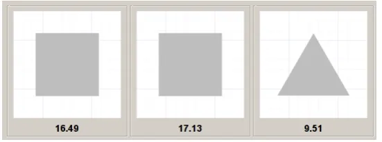
An example of a menu with three elements and a common standard (the triangle) is
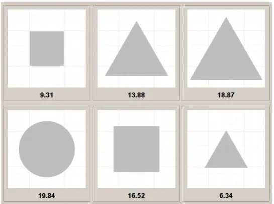
shown in figure 1. An example of a menu with six elements and no common standard is
[image:9.595.161.437.427.530.2]shown in figure 2.
Figure 2: Screen shot of a menu with six offers and no common standard.
Each individual was faced with 80 menus, the same set for everyone but presented in a
subject-specific random order. 36 menus showed three options (“3-menus”), of which 18
with one CS. 44 showed six options (“6-menus”), of which 18 with one CS and 8 with two CS
(one CS with two members, the other CS with three). In each case, half of the menus were
hard (σ2 = 0.01) while the other half were easy (σ2 = 0.05). The distribution of menus is
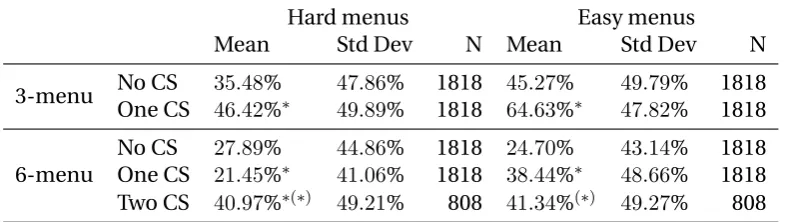
summarized in table 1.2
Table 1: Distribution of menus by CS and difficulty of the problem.
Hard menus Easy menus
(σ2 = 0.01) (σ2= 0.05)
3-menu No CS 9 9
One CS 9 9
6-menu
No CS 9 9
One CS 9 9
Two CS 4 4
Given the random process governing unit price generation, the lowest priced common
standard offer had a theoretical chance of being the optimal choice in 23of our 3-menus with
a CS, in 13of our 6-menus with one CS and in36of our 6-menus with two CS (considering only
the lowest priced of the CS with 3 options). The actual realization of these chances was56%
in 3-menus,39%in 6-menus with one CS and63%in 6-menus with 2 CS.
The participants had up to two minutes to choose an offer from each menu and were
2The menus are available for visual inspection at https://people.econ.mpg.de/
[image:10.595.176.420.489.602.2]forced to spend a minimum time of10 seconds on each menu. The choice was performed by clicking on an offer - in which case it would be highlighted with a light green frame - and
could be revised as many times as one wanted within the two minutes limit. The choice was
finalized by clicking on a ’Submit’ button at the bottom of the screen. If no final choice was
submitted within the time limit the last highlighted offer was submitted as the final choice;
if no offer had been highlighted, then the participant received a payment of3euros for that
trial, which was less than the minimum payment a participant could get even if he made the
worst choice out of all our menus.3
The participants were given feedback after each menu. This feedback reminded them of
the price of their chosen offer, told them the resulting expenditure to paintA, as well as their
payoff in terms of budget minus expenditure. The participants were not given the possibility
to automatically store and retrieve their payoffs from previous rounds, but were provided
with pencil and paper and some did record their payoffs. After the feedback dialog, they were
given a new budgetBand shown the next menu. The participants knew the total number of
menus was 80 and were reminded of their progress along the experiment.
1.2 Control tasks
Once finished with the main task, the participants were exposed to a set of non-incentivized
visual perception and computational skills tasks to control for their ability to perform the
main task. No minimum time was enforced and the participants could skip any question
within each task.4 Three different set of tasks were chosen:
1. Shape size comparisons: The participants were asked to give their estimate of the
rela-tive size of a shape (rectangles, circles and triangles) with respect to another. Each of
four comparison had to be done within a time limit of one minute.
2. Mathematical operations. The participants were asked to solve three sets of 10
oper-ations (sum, subtraction, multiplication, divisions).5 Each set had to be completed
within one minute.
3. Simple problems: The participants were asked to solve four simple problems, testing
3Only one participant failed to submit a decision within the time limit, and this only once, in that case
high-lighting no offer.
4Only one participant did so.
5The sets were generated using Mail Goggles’s GMail Labs app by Jon Perlow and were graded in terms of
their understanding of the concept of area, of how an area relates to its dimensions,
and how a number can be translated from one standard to another (here, a currency).
Each problem had to be solved within two minutes.
Once done with the control tasks, the participants filled in a short demographic
question-naire. They were finally asked to guess what the experiment was about - to check for demand
effects - and to rate their level of motivation during the experiment. Finally, each participant
individually drew a number from 1 to 80 from an urn and was paid according to the result of
her purchasing decision in the period corresponding to that number.
Our whole experiment was computerized. The experimental software, the menu
genera-tor and the script we used to collect and organize the raw data were programmed in Python
(van Rossum, 1995).6The German instructions, as well as their English translation, are
avail-able upon request.
2
The common standard rule and its generalization
In his choice, the consumer may take into account a number of criteria involving the
per-ceived unit prices of offers, their shape, their position and their belonging to a CS. Let us
consider how a consumer might go about a “covert sequential elimination process” as per
Tversky (1972), based on perceived unit price and belonging to a CS. Denoteupˆij =upi+eij
the perceived unit price of offeriby consumerj (the “signal”). upi is the unit price of offer
i, whileeij is an error term, which is independent across offers in a menu and across
con-sumers. How large the error term will be on average will depend on the consumer’s accuracy
and on how difficult it is to compare offersacrossstandards. As for whether an offer belongs
to a CS or not, this matters because prices are directly comparablewithina standard, so the
consumer can identify the Lowest Priced Common Standard offer (“LPCS”) with high
accu-racy.7 A consumer who only considers signals for his choice will choose the offer with the
lowest signal and will not consider whether that offer may be dominated by another offer
expressed in terms of the same standard. This is what we call theNaive rule. A variant on
6Different python modules were needed to develop the experimental software: wxpython was used for the
graphical user interface, and two community-contributed packages, svgfig and polygon, were used for creating and managing the shapes. The experimental software (menu and shape generators and analyzers, user interface) and its documentation, as well as the raw data and the script used to collect and organize them are available upon request.
7We will consider the possibility that a consumer may make mistakes in choosing among CS even if he is
the Naive rule adds a second step whereby the consumer checks if the offer he chose after
the first step based on signals may not be dominated by another offer expressed in the same
standard, and if so, revises his choice to the dominant offer. This is what we call theSignal
Firstheuristic. The reverse steps,i.e.first eliminate dominated offers within a standard, and
then compare the dominant CS offers with those expressed in terms of an IS based on their
signal, is calledDominance Editing. Finally, a rule based only on belonging to a CS, which
we call theCS rule, consists in choosingarg min
i∈CS
pi(the LPCS) if a CS exists and revert to the
Naive rule otherwise. The consumer not only avoid the higher priced of the common
stan-dard offers but choose the LPCS and disregard individuated stanstan-dard (“IS”) offers. There are
many reasons why we would expect consumers to follow such a rule:
1. Statistically, if one assumes that prices are i.i.d. across offers and offers are assigned to
a CS at random, then the LPCS is lower priced in expectation than other offers. As in
the Monty-Hall problem (Friedman, 1998), there is information gained from being told
that an option is dominated.
2. Behaviorally, consumers have been shown to be subject to the asymmetric dominance
effect (Ariely, 2008, Chapter 1), so that when faced with three offers, one being
domi-nated by another, that other will be chosen more often than if the domidomi-nated offer was
not present. Another way to call this effect in the field of decision theory is the
“attrac-tion effect”, which is a type of context effect (Huber and Puto, 1983).
3. From learning: Gaudeul and Sugden (2012) argue that consumers are better off
choos-ing among CS offers when firms are strategic agents in a competitive settchoos-ing, subject to
at least some agents following the CS rule. This learning is made easier by the
appli-cability of the common standard rule to many environments, so that consumers who
learned from one environments that CS offers are lower priced than other offers will
apply this insight generally. Consumers ought therefore to learn to choose CS offers
over time (Sugden, 1986; Fudenberg and Levine, 1998).
4. For simplicity, as agents faced with complex choices tend to follow simple heuristics,
often with good results (Gigerenzer and Brighton, 2009). In this case, an offer being
un-ambiguously better than another provides “one good reason” to choose it (Gigerenzer
The CS rule, based on multiple foundations, can thus be generalized across many settings
and is likely to be more robust than rules that hold only in some settings (Sugden, 1989) or
that can be justified in only one way. We believe this rule is at work in a wide variety of
con-sumer choice problems. Its simplicity and intuitive appeal make it particularly interesting for
economists interested in consumer behavior and heuristics, marketing, consumer
protec-tion and the competitive process. Note that we are not wedded to one particular explanaprotec-tion
for why consumers might prefer CS offers: we are only interested in determining if they do so
and if so, to what extent. Indeed, the main reason we are interested in this possible consumer
bias is that we believe that it could drive firms into making their offers less difficult to
com-pare and thus encourage the efficient working of competitive markets. Our setting provides
a lower bound for the CS effect, in so far as any competitive effect justifying the use of the
rule is excluded by design since offers are not determined through a competitive process.
The Threshold rule. Following the CS rule is strictly optimal in the context of Gaudeul and
Sugden (2012) as IS offers are systematically higher priced than CS offers in a competitive
setting where firms can choose their standard, so that even an IS offer with a very good
signal should be rejected. However, the CS rule is not optimal in the context of our
ex-periment as offers are randomly generated rather than the result of a competitive process.
It is better for a consumer to follow a more generalThreshold rule, which we present
be-low, in our setting. The Threshold rule functions as follows: determine the LPCS, denoted
k≡arg min
i∈CS
piif there is a CS and then choosel(vj) = arg min
i /∈CS
( ˆupk,upˆi×vj),i.e. the price of
all IS options is multiplied byvj, withvj depending on consumerj’s preference for (vj > 1)
or against (vj < 1) the LPCS. We will callvj a threshold and the optimal choice of
thresh-old isv∗
j = arg min vj
E(upl(vj)). Its level depends on the consumer’s accuracy in assessing the
unit price of offers in a menu, with less accurate consumers benefiting from adopting higher
thresholdsvj. Thresholdvj = 1corresponds to eliminating dominated offers and choosing
based on the signals from the remaining offers (this is Dominance Editing), while threshold
vj → ∞corresponds to the CS rule.
To put this in behavioral terms, the consumer who adopts a thresholdvj > 1does not
reject IS offers out of hand, but penalizes them, that is, he does not follow his first
impres-sion (upˆij) of the price of the IS offer, but rather revises it upwards when comparing it to his
certain dose of skepticism to his evaluation of an offer that is expressed in uncommon terms,
and will choose to buy it only if it seems sufficiently better than the best of those offers that
are expressed in common terms – that is, if its unit price appears to be lower by a factor of at
least1−1/vj compared to the apparent unit price of the LPCS.
To make this clearer, let us come back to the example on page 2. We saw that under the CS
rule, the consumer would always choose the orange. Under the Threshold rule, the consumer
will choose the orange only if his thresholdvis more than1.29/1.27 = 1.016.
A consumer’s optimal threshold depends on his accuracy in assessing offers, with less
accurate consumers being better off adopting higher thresholds. For example, a consumer
who makes considerable mistakes obtainsB−E(a)in expectation under the Naive rule (he
chooses essentially at random), which is less thanB−E(min(a, b)), his expected payoff under
the CS rule.
We performed simulations with Octave (Eaton, 2002) to determine the optimal threshold
vto use under the Threshold rule as a function of consumers accuracy.8 We modeledeij as
following a normal distribution with mean zero and varianceσ2, which we varied between0
and0.2. In the same way as in our experiment, products unit pricesupi followed a normal
distribution with mean0.5and variance0.01(hard menus), and0.05(easy menus) andBwas
set to60. Consumer choice was simulated according to the Naive rule as well as according
to the Threshold rule, with the optimal threshold v calculated for every level ofσ2 — less
accurate consumers benefit from adopting higher thresholds. Their average payoff for each
rule was calculated over2million menu draws so as to achieve good accuracy.9
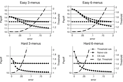
The following graphs show payoffs in the four situations in our experimental setting, that
is depending on whether the consumer has a choice among three or six options, and whether
menus are easy or hard. Also shown on a separate scale is the optimal thresholdv∗
for each
value of the error term.
8Program available upon request.
9The ranking of payoffs by rules is quite robust as differences in payoffs are significant even for much smaller
1 1.2 1.4 1.6 1.8 2 Threshold 10 11 12 13 14 15 16 17 Payoff
0 .05 .1 .15 .2
error Easy 3-menus 1 1.2 1.4 1.6 1.8 2 Threshold 10 11 12 13 14 15 16 17 Payoff
0 .05 .1 .15 .2
error Easy 6-menus 1 1.2 1.4 1.6 1.8 2 Threshold 10 11 Payoff
0 .05 .1 .15 .2
error Hard 3-menus 1 1.2 1.4 1.6 1.8 2 Threshold 10 11 Payoff
0 .05 .1 .15 .2
[image:16.595.91.504.76.352.2]error Threshold rule Naive rule CS rule Opt. Threshold Hard 6-menus
Figure 3: Consumer payoffs by choice rules and optimal thresholds, by menu length and difficulty.
As can be seen in figure 3, payoff decreases as consumers become less accurate in their
choice (higherσ2), except for the CS rule since consumers always choose correctly among CS
offers and thus obtainB −E(min(a, b)). The Threshold rule outperforms the CS and Naive
rules and converges towards the CS rule for less accurate consumers as can be seen from the
rising level of the optimal thresholdvasσ2increases. Following the CS rule obtains higher
payoffs than the Naive rule as long as consumers are not too accurate. This is so especially
when menus are hard as then even high levels of accuracy may result in mistakes. From this
graph, one can infer a consumer’s accuracy from the average payoff he attained when facing
menus with no common standard, and from this accuracy determine the threshold he ought
to use when facing offers with a CS.
Other possible influences on consumer choice. Consumers may be subject to other
influ-ences in their choices and we will need to control for those. Biases may come from following
alternative possible rules as follows:
equiva-lently lower priced items. While this does not make sense in our setting, this rule may
be imported from other settings where for example the consumer faces a binding
bud-get constraints (Viswanathan et al., 2005). Alternatively, abulk purchasing rule would
favor big packages, as offers in big packages are usually better deals than those in small
packages.
• Thelexicographic rulemay favor the first offers in the lexicographic order in the menu
– maybe because the consumer is satisficing rather than optimizing (Simon, 1955) or
simply because he does not have time to consider all offers. Alternatively, a consumer
may also favor the last offers in the menu if he tends to remember (and choose) the last
option he read from a list.
• Finally, consumers may favor some shapes over others because they appear larger, as
evidenced in Krider et al. (2001). As evoked before, broad based offers such as triangles
will be preferred to squares covering the same area and those will be preferred to the
compact circle offers.
3
Results
Our experiment took place at the laboratory of the Max Planck Institute in Jena in June 2011.
The experiment involved 202 students over 8 sessions, each with 24 to 27 subjects. Our
sub-jects were asked for their age, gender, field of study, year of study, motivation in completing
the tasks, and also what they thought the experiment was about (in order to control for
de-mand effects). All subjects were students. When asked what they thought the experiment
was about after going through it, most subjects guessed we wanted to assess their abilities
to take account of both price and area to identify the best offer in our menus. Some
won-dered if we wanted to identify what shapes were perceived as more attractive, but no subject
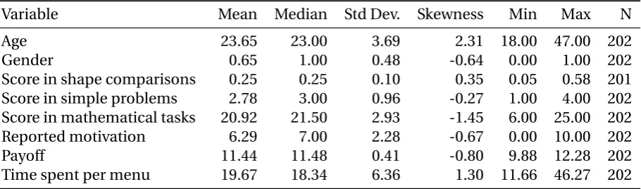
Table 2: Summary statistics.
Variable Mean Median Std Dev. Skewness Min Max N
Age 23.65 23.00 3.69 2.31 18.00 47.00 202
Gender 0.65 1.00 0.48 -0.64 0.00 1.00 202
Score in shape comparisons 0.25 0.25 0.10 0.35 0.05 0.58 201
Score in simple problems 2.78 3.00 0.96 -0.27 1.00 4.00 202
Score in mathematical tasks 20.92 21.50 2.93 -1.45 6.00 25.00 202
Reported motivation 6.29 7.00 2.28 -0.67 0.00 10.00 202
Payoff 11.44 11.48 0.41 -0.80 9.88 12.28 202
Time spent per menu 19.67 18.34 6.36 1.30 11.66 46.27 202
The average age of our subjects was 24, ranging from 18 to 47 (Table 2). 65% of our
sub-jects were women. The average motivation of our subsub-jects, on a scale from 0 to 10, was 6,
with a median motivation of 7 and 75% of our subjects having motivation more than 5, the
middle point. The monotony of the tasks did not therefore result in noticeable discontent.
Speed of choice for each menu and each subject was also recorded. Subjects took 20
sec-onds on average to make each choice (they could not make a choice before 10 secsec-onds had
elapsed). Time spent on each menu was longer for menus with more options and declined
over time (from an average of 36 seconds for the first choice to 16 for the last).
There were three control tasks. In the shape comparison task, we computed individual
performance as the average of|guess−true value|/true value. On average, people were 25%
off the true value, with a minimum of 5% and a maximum of 58%. In the mathematical tasks,
we coded answers as either right or wrong. On average, subjects got 21 of the 25 calculations
right, with only two obtaining less than half of the calculations right, and 7 of them obtaining
all of them right. Finally, in the simple problems, only about 62% answered more than half
of the questions correctly. Performance in the different control tasks were significantly and
positively correlated, though not highly (correlation coefficients were around 0.35). Women
performed less well than men in all control tasks.
3.1 Did individuals benefit from the presence of a common standard?
Overall, consumers made about 39% of their choices optimally, that is, choosing the offer
the optimal choice. In other terms, most consumers were wrong for most menus.10 Table 3
shows how often consumers made the optimal choice depending on the length of the menu,
its difficulty and whether the menu included one CS, two CS or no CS. The presence of a CS
significantly improved accuracy in consumer choices, except in the case of hard 6-menus.
Consumers were also more likely, as designed, to choose the best option when the menu was
[image:19.595.102.495.242.353.2]easy.
Table 3: Optimal choices by menu length, difficulty and presence of a CS.
Hard menus Easy menus
Mean Std Dev N Mean Std Dev N
3-menu No CS 35.48% 47.86% 1818 45.27% 49.79% 1818
One CS 46.42%∗ 49.89% 1818 64.63%∗ 47.82% 1818
6-menu
No CS 27.89% 44.86% 1818 24.70% 43.14% 1818
One CS 21.45%∗ 41.06% 1818 38.44%∗ 48.66% 1818
Two CS 40.97%∗(∗) 49.21% 808 41.34%(∗) 49.27% 808
* Difference significant at 5% levelvs.one row above, Wilcoxon rank-sum test. (*) Difference significantvs.two rows above.
We did not find any effect of the presence of a CS in a menu on the speed with which
consumers took a decision, except in the case of easy 3-menus where the presence of a CS
reduced time spent from 18 to 16 seconds on average. Subjects took on average 5 seconds
more to reach a decision among 6-menus than among 3-menus, but did not reach faster
decisions when the menu was easy (except again in the case of easy 3-menus).
Let us now consider whether higher accuracy in choices led individuals to obtain higher
payoffs when a menu included CS offers. The following table displays individual payoffs by
menu length, difficulty and presence of a CS (Table 4).
10Looking at menus where consumers performed particularly badly, one finds that they mistakenly chose
Table 4: Payoffs by menu length, difficulty and presence of a CS.
Hard menus Easy menus
Mean Std Dev N Mean Std Dev N
3-menu No CS 10.41 0.92 1818 11.02 4.56 1818
One CS 10.45 0.96 1818 13.34∗ 3.96 1818
6-menu
No CS 10.14 0.81 1818 11.97 4.11 1818
One CS 10.04∗
0.98 1818 13.84∗
5.48 1818
Two CS 10.78∗(∗) 0.87 808 12.78(∗) 4.34 808
* Difference significant at 5% levelvs.one row above, Wilcoxon rank-sum test. (*) Difference significantvs.two rows above.
This table can be read in conjunction with another table that indicates how those
pay-offs translate in terms of how close they are to the maximum available payoff in each menu.
Table 5 thus reports the average of the ratio(upmax −upchosen)/(upmax −upmin)over
individuals and menus in each category. We normalize the difference between the worst
choice and the consumer’s choice as shown because we want to be able to compare
perfor-mance between easy and hard menus, where the difference between the worst and the best
choice within a menu will be smaller on average. We call this the performance ratio. A value
of0would indicate the consumers always made the worst choice, while a value of1would
[image:20.595.105.490.505.615.2]indicate they always made the best choice.
Table 5: Performance ratio by menu length, difficulty and presence of a CS.
Hard menus Easy menus
Mean Std Dev N Mean Std Dev N
3-menu No CS 0.597 0.447 1818 0.607 0.448 1818
One CS 0.592 0.419 1818 0.794∗
0.324 1818
6-menu
No CS 0.683 0.353 1818 0.682 0.321 1818
One CS 0.545∗
0.364 1818 0.735∗
0.299 1818
Two CS 0.735∗(∗) 0.323 808 0.759∗(∗) 0.365 808
* Difference significant at 5% levelvs.one row above, Wilcoxon rank-sum test. (*) Difference significantvs.two rows above.
Subjects obtained a payoff of 11.44 ECU on average (1 ECU=0.8=C), and their performance
ratio was 0.66. No participant obtained payoffs that were significantly less than 10.22, which
is what they would have obtained had they chosen at random within our menus, and only
8 obtained payoffs that were not significantly greater than this. Subjects therefore seem to
obtained higher payoffs with 6-menus and with easy menus.
Participants obtained significantly higher payoffs and performed significantly better when
a menu was easy and included a CS, while the effect of the presence of a CS in hard menus
was either not significant or slightly negative. The presence of a CS did not therefore
bene-fit consumers when prices were already close together, but worked to the advantage of
con-sumers when prices varied more widely among options, which would be the case when firms
are not in close competition. The CS effect would therefore be at play when it matters most.
Panel regressions of payoffs on individual and menu characteristics are shown inTable 11
on page 36. A Breusch and Pagan Lagrange multiplier test for random effect indicates that
there are no significant difference across units so that one can rely on the results of a pooled
regressions (OLS). Compared to the base case (Easy 3-menus with no CS), individuals
ob-tained higher payoffs when the menu displayed 6 options and when the menu included CS
offers. Payoffs were smaller when the menu was hard. Looking at cross-effects, one sees that
making a 6 menus harder negates the benefit of having more choice, and making a menu with
a CS harder negates the benefits of having a CS. Finally, the gain from including CS offers in
a 6-menu are mainly due to the presence of a CS rather than from having more options.
In-dividuals improved their payoffs with experience (“order” variable). Older people obtained
lower payoffs, while those with higher scores in the mathematical and practical
consump-tion problems, or with higher motivaconsump-tion, obtained higher payoffs. Time spent choosing an
offer within each menus did not appear to have a significant effect overall, though
individu-als who spent more time on average obtained higher payoffs (cf.between effects regression)
while they obtained lower payoffs on those tasks on which they spent more time than their
average (cf. fixed effects regression).11 There was no sign of a significant individual effect,
that is, no individual seemed to perform better than others above and beyond what could be
predicted from their gender and scores in control tasks. We also checked that there was low
correlation between residuals and variables in the model.
11We checked also if there was some quadratic effect in terms of time spent. Indeed, time spent could increase
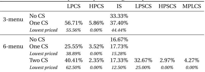
3.2 Did individuals favor the lower priced of the common standard offers?
Table 6 shows that the LPCS was chosen about 57% of the time within our 3-menus,12about
as often as the LPCS was the lower priced product (56%). This was less often than if
con-sumers followed the CS rule, whereby the LPCS would always be chosen. However, the IS
was disfavored as it was chosen less often than if consumers always chose the lowest priced
product (37% of the time while it was the lowest price in 44% of the menus). In the case of
6-menus with one CS, the LPCS was chosen about 26% of the time in 6-menus with only one
CS, which was less often than optimal (39%). The IS on the other hand was chosen more
of-ten than optimal (18% vs. 15%). Finally, the lower priced of the larger CS (the one with three
members) was chosen more often than the lower priced of the smaller CS in 6-menus with
two CS, (40% vs. 33%), but less often than optimal (62%), and the IS was chosen more often
[image:22.595.99.498.367.508.2]than optimal.
Table 6: Choice frequencies by menu length and presence of a CS.
LPCS HPCS IS LPSCS HPSCS MPLCS
3-menu No CS 33.33%
One CS 56.71% 5.86% 37.40%
Lowest priced 55.56% 0.00% 44.44%
6-menu
No CS 16.67%
One CS 25.55% 3.52% 17.73%
Lowest priced 38.89% 0.00% 15.28%
Two CS 40.41% 2.35% 17.33% 32.67% 2.97% 4.27%
Lowest priced 62.50% 0.00% 12.50% 25.00% 0.00% 0.00%
Notes: In the case of 6-menus with two CS, the LPCS is the Lower Priced of the Larger CS (the one with three members), the HPCS is the Higher Priced of the Larger CS, and the MPLCS is the Middle Priced of the Larger CS. The LPSCS is the Lower Priced of the Smaller CS (the one with two members) and the HPSCS is the Higher Priced of the Smaller CS. In 6-menus with one CS,
the IS choice frequency is calculated by averaging across the four IS offers.
In the aggregate, consumers do not appear to follow a Naive rule since most of them took
account of the presence of a CS by discarding higher priced CS offers. The LPCS was chosen
more often than any other offer. A number of consumers appear to have avoided IS offers
in 3-menus although higher sales by the LPCS in 6-menus appear to have occured mainly
because of diversion away from the dominated CS offer rather than because consumers
con-sistently avoided IS offers. All the same, even in that case, diversion was mainly towards
lower priced common standard offers rather than sales being equally distributed across IS
and LPCS.
Figure 5 on page 37 displays the distribution of the frequency with which individuals in
our sample chose the lower priced of the common standard offers. This is disaggregated by
menu length and difficulty, and by whether the menu included one or two CS in the case of
6-menus. In each graph, the first reference line to the left indicates the proportion of choices
of the LPCS that would be consistent with consumers following a Naive rule, i.e. choosing
among options as if there was no CS. In the case of 3-menus, this corresponds to 33%, and
in the case of 6-menus to 17%. The second reference line corresponds to the proportion of
choices of the LPCS that would be consistent with consumers doing Dominance Editing, that
is, eliminating the dominated CS offer and comparing the LPCS with the IS offers. This would
lead the LPCS to be chosen 50% of the time in 3-menus, 20% of the time in 6-menus with one
CS and 33% of the time in 6-menus with two CS. The third reference line corresponds to the
proportion of choices of the LPCS that would be consistent with consumers following the
Signal First heuristic, that is, first assessing options based on their signal, and then
trans-ferring their preliminary choice of a dominated CS offer onto the LPCS. This would lead the
LPCS to be chosen 67% of the time in 3-menus, 33% of the time in 6-menus with one CS and
50% of the time in 6-menus with two CS (for the CS with more options). Like the CS and the
Threshold rule, the Signal First heuristic thus results in the LPCS gaining a large advantage on
IS offers. Anybody to the left of the first reference line can be said to disfavor CS offers, those
between the two first reference lines do not either favor or penalize CS offers while those to
the right of the last reference line can be said to favor CS offers vs. IS ones. One sees that a
significant proportion of subjects favor the LPCSvs.the IS offer in 3-menus, especially if the
menu is easy. However, the proportion of such consumers is smaller in 6-menus with a CS.
Preference for the LPCS in 6-menus with two CS is more pronounced.
One cannot however rely on such descriptive statistics to assert with certainty that a
por-tion of consumers favored CS offers, since the results we showed could be due to chance. Our
random draw of offers, their price, shape, size, position in the menu, could be the driver
be-hind our results. This is why we perform regressions that are designed to correct for possible
biases due to the elements mentioned above.
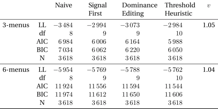
Predicting consumer choice when there is a common standard. We perform maximum
likelihood estimation with three different models of consumer choice among option: the
al-lows for preference heterogeneity for all the attributes. The probit model is fitted by using
maximum simulated likelihood implemented by the Geweke-Hajivassiliou-Keane (GHK)
al-gorithm (Greene and Hensher, 2003). The Halton sequence is used to generate the point sets
used in the quasi-Monte Carlo integration of the multivariate normal density, while
opti-mization is performed using the Berndt-Hall-Hall-Hausman procedure (Berndt et al., 1974).
The mixed logit model is fitted by using maximum simulated likelihood (Train, 2003) and the
estimation was performed with the user-writtenmixlogitcommand for Stata (Hole, 2007).
Estimation makes use of the sandwich estimator of variance, except when performing the
probit regressions with 6-menus as convergence was not achieved otherwise.
The outcome for each menu is one of 3 or 6 options. Options are identified by their
posi-tion in the menu, and by whether they are the LPCS, HPCS or an IS in menus with a CS. The
dependent variable is the choice of the consumer among alternatives and the independent
variables include the unit price of the option, its shape, its size and its position. Since shapes
that extend more broadly in space are preferred (see Krider et al., 2001), we create a variable
coding shapes from most to least attractive: a triangle is assigned a value of 1, a square a
value of 2 and a circle a value of 3.13 The variable “position” is coded by lexicographic
posi-tion in the menu, from 1 if the opposi-tion is in the top left corner to 6 if it is in the bottom right
corner in a 6-menu, otherwise to 3 for the option to the right in a 3-menu. As per a remark in
Hole (2007), we include no alternative-specific constants in our models, which is “common
practice when the data come from so-called unlabeled choice experiments, where the
alter-natives have no utility beyond the characteristics attributed to them in the experiment.” We
will also cross unit price with case specific variables such as gender and scores in the control
tasks to determine whether individual characteristics make our subjects more or less
sensi-tive to price signals (other individual characteristics such as age and educational background
do not vary sufficiently in our sample). We also consider a menu specific variable (whether
the menu was “hard” or “easy”) and variables that are both menu and case specific (the order
in which a specific menu was presented to an individual and the time that individual spent
deciding on this menu).
Whether a subject avoids the HPCS or prefers the LPCS vs. the ISs may depend on their
individual characteristics so that we introduce case-specific variables (here, a case is an
in-dividual) along with alternative-specific variables to determine choice among alternatives.
Our case specific variables are scores in the mathematical, shape comparison and simple
problems, along with gender, time spent choosing within a menu and motivation. We also
consider whether facing a hard menu makes it more likely to favor the LPCS as following a
simple heuristic may be more likely if there appears to be little difference in prices between
options. Finally, we consider whether the LPCS was next to the HPCS on the same row in the
menu since it is easier to notice there is a CS if CS options are close together.
Formally, denoteyo
ijmthe utility of optionjin menumfor individuali, and denoteyijm=
1if that option is chosen. We will haveyijm = 1ifyoijm > yitmo for allt6=jin menum,0else.
Latent utilityyo
ijmtakes the formyijmo =α upjm+ω×upjm×Ωi+µ×upjm×Mm+λj×Ωi+
θj×Mm+βshapejm+γsizejm+φpositionjm+uijm. An option is coded in terms of whether
it is the LPCS, the HPCS or an IS offer.Ωiis aq×1vector of case-specific variables, the same
variables being assumed to influence the choice for each option,ωis a1×qvector of
param-eters,Mmis ah×1vector of menu-specific variables whileµis a1×hvector of parameters.
λjis a1×qvector of parameters, different for each alternative as case-specific variables are
assumed not to influence the choice of each alternative in the same way. Similarly,θj is a
1×hvector of parameter translating the influence of menu characteristics on the choice of
an alternative. uijmis a random variable of mean0that follows either a logistic or a normal
distribution. We constrainλj andθj to be the same for all four IS options in 6-menus with
a CS. Model selection using the AIC finds that all of the alternative specific variables ought
to be used, while only score in the shape comparison and in the mathematical tasks, along
with gender and whether a menu is hard or easy, ought to be used as case-specific variables.
Table 7: Regressions with a CS, 3 and 6-menus.
(1) (2) (3) (4) (5) (6) (7) (8) (9)
Logit 3-menus Probit 3-menus MixLogit 3-menus Logit 6-menus Probit 6-menus MixLogit 6-menus Logit 6-m 2 CS Probit 6-m 2 CS MixLogit 6-m 2 CS
main unit price (up) −14.5806∗ ∗∗ −9.5842∗ ∗ −15.5821∗ ∗∗ −19.2308∗ ∗∗ −6.9231∗ ∗∗ −19.6781∗ ∗∗ −11.6973∗ ∗∗ −1.9796 −12.2147∗ ∗∗ (−4.99) (−2.71) (−4.65) (−11.03) (−4.85) (−9.62) (−4.09) (−0.28) (−3.63) up×shape task −5.0589 −4.1344 −5.2897 17.5590∗ ∗ 5.8729∗ 18.0310∗ 6.4474 1.0936 7.1735
(−0.48) (−0.61) (−0.45) (2.85) (2.53) (2.49) (0.64) (0.27) (0.59) up×hard menu 16.4312∗ ∗∗ 10.9950∗ ∗ 16.8252∗ ∗∗ 15.0242∗ ∗∗ 4.7505∗ ∗∗ 16.0361∗ ∗∗ 8.8646 −1.2748 10.2190
(3.90) (3.29) (3.44) (4.72) (3.44) (5.17) (0.88) (−0.25) (0.99) position −0.0543+ −0.0463+ −0.0489 0.0696∗ ∗∗ 0.0325∗ ∗∗ 0.0656∗ ∗∗ 0.0205 0.0028 0.0303
(−1.75) (−1.94) (−1.59) (6.42) (3.94) (6.08) (0.84) (0.21) (1.16) shape −0.2062∗ ∗∗ −0.1465∗ ∗ −0.2333∗ ∗∗ −0.3682∗ ∗∗ −0.1332∗ ∗∗ −0.4286∗ ∗∗ −0.6777∗ ∗∗ −0.0766 −0.7630∗ ∗∗
(−5.21) (−2.61) (−4.96) (−14.56) (−4.84) (−10.18) (−9.49) (−0.28) (−10.17) size −0.0007 −0.0004 0.0009 −0.0058∗ ∗ −0.0019∗ −0.0062+ −0.0447∗ ∗∗ −0.0036 −0.0370∗ ∗∗
(−0.21) (−0.16) (0.20) (−3.21) (−2.04) (−1.70) (−5.87) (−0.28) (−3.73) HPCS score shape task 1.9492∗ 1.4973∗ ∗ 1.9687∗ 2.7203∗ 1.1523∗ ∗ 2.7527∗ −0.1989 0.0525 −0.2176
(2.44) (2.73) (2.12) (2.48) (2.78) (2.45) (−0.12) (0.04) (−0.12) score math −0.0096 −0.0113 −0.0090 0.0675+ 0.0239 0.0689+ −0.0776+ −0.0508 −0.0756
(−0.41) (−0.69) (−0.30) (1.87) (1.61) (1.85) (−1.71) (−0.97) (−1.41) gender −0.4832∗ ∗ −0.2882∗ ∗ −0.4819∗ −0.8498∗ ∗∗ −0.3015∗ ∗∗ −0.8506∗ ∗∗ −1.3970∗ ∗∗ −0.8411∗ −1.3944∗ ∗∗
(−3.24) (−2.74) (−2.43) (−4.30) (−3.43) (−3.66) (−4.06) (−2.45) (−3.71) hard menu −0.1681 −0.1401 −0.1995 −0.5105∗ −0.0970 −0.5341∗ ∗ −0.3825 0.2909 −0.4529
(−1.03) (−0.90) (−1.34) (−2.55) (−1.08) (−2.58) (−0.94) (0.61) (−1.10) close CS −0.4200+ −0.1512 −0.4122∗ −0.1289 0.0471 −0.1133 −0.2745 −0.4255 −0.2341
(−1.95) (−0.97) (−1.98) (−0.50) (0.46) (−0.45) (−0.78) (−1.03) (−0.61) constant −1.5065∗ −1.7151∗ ∗∗ −1.4918∗ −2.9550∗ ∗ −1.7752∗ ∗∗ −2.9806∗ ∗ 0.2745 −1.1791 0.2397
(−2.42) (−3.67) (−1.97) (−3.25) (−3.40) (−3.23) (0.22) (−0.73) (0.16) IS score shape task −0.2998 −0.3094 −0.4166 0.0294 0.1489 0.0205 0.1574 0.0123 0.1212
(−0.77) (−1.07) (−0.94) (0.06) (0.87) (0.04) (0.18) (0.11) (0.15) score math 0.0248+ 0.0188+ 0.0284 0.0054 0.0016 0.0062 0.0078 0.0004 0.0103
(1.84) (1.74) (1.54) (0.37) (0.27) (0.36) (0.29) (0.13) (0.30) gender −0.2679∗ ∗∗ −0.1628∗ −0.3129∗ ∗ −0.2517∗ ∗ −0.1132∗ ∗ −0.2657∗ ∗ −0.3562∗ −0.0368 −0.3590∗
(−3.45) (−2.23) (−3.18) (−2.80) (−2.78) (−2.69) (−2.30) (−0.28) (−2.25) hard menu 0.0105 −0.0190 −0.0386 −0.4933∗ ∗∗ −0.1580∗ ∗∗ −0.4923∗ ∗∗ 0.6969∗ ∗ 0.0083 0.5104∗
(0.13) (−0.34) (−0.45) (−5.46) (−3.43) (−5.51) (3.03) (0.15) (1.96) close CS −0.7851∗ ∗∗ −0.5384∗ ∗ −0.8847∗ ∗∗ 0.2557∗ 0.0519 0.2872∗ ∗ 0.4785∗ ∗ −0.0070 0.6749∗ ∗
(−6.39) (−2.94) (−7.38) (2.36) (1.16) (2.65) (2.65) (−0.22) (3.21)
close SCS −0.2762 0.0985 −0.2752
(−0.69) (0.27) (−0.71) constant 0.0291 −0.0573 0.0736 0.1316 0.0202 0.0741 −1.2370+ −0.0573 −1.3206
(0.08) (−0.23) (0.15) (0.35) (0.13) (0.17) (−1.73) (−0.25) (−1.53)
SD shape 0.3763∗ ∗∗ 0.4722∗ ∗∗ 0.2567∗
(7.63) (10.60) (2.38)
size 0.0363∗ ∗∗ −0.0428∗ ∗∗ 0.0650∗ ∗∗
(8.18) (−11.42) (7.39)
N 10851 10851 10851 21708 21708 21708 9648 9648 9648
ll −2919.5938 −2917.2251 −2850.6984 −5617.2643 −5564.1585 −5450.2711 −2078.6207 −2057.6991 −2055.1065
tstatistics in parentheses +p <0.10, *p <0.05, **p <0.01, ***p <0.001
In terms of alternative-specific variables, subjects tend to prefer lower priced options,
“broader” shapes, and smaller sized options (equivalently, those with lower displayed prices).
One can notice that prices being close together (hard menus) makes consumers less sensitive
to price. Case-specific variables show that consumers tend to avoid the HPCS: the parameter
on the constant term for that option is negative and highly significant. Individuals that are
worse at the shape comparison tasks are more likely to choose the HPCS, maybe because
they find it difficult to compare the area and shape of all options and thus do not notice the
presence of a CS. It is however only women who display an aversion to the ISvs. the LPCS.
Aversion to the IS is encouraged when the presence of a CS is more obvious, i.e. when the CS
options are next to each other – there is a negative impact of the dummy variable taking value
one if CS options are close in 3-menus (the impact is not consistent across logit and probit
regressions in the case of 6-menus). Whether the menu is hard also encourages individuals
in rejecting the IS option, at least in 6-menus with one CS (results in the case of 6-menus with
two CS are not consistent across logit and probit regressions).
In conclusion, only women appear to favor the LPCS when choosing among options. This
might explain why women managed to obtain higher payoffs than men in this experiment
even though they were less good at those control tasks that predicted higher payoffs.
3.3 How strong was the common standard effect?
It is difficult to quantify the strength of the Common Standard effect from the results
pre-sented up to now. We seek to know how much of an advantage a LPCS offer gains compared
to an offer expressed in terms of an individuated standard. We simulate in this part how
con-sumers would make choice among menus with a CS based on their choices when there is no
CS. We first perform regressions to explain consumer choice when there is no CS, and then
apply predictions from that setting to the case where there is a CS, assuming consumers
ap-ply the Threshold rule. We determine what thresholds best predicts consumer choice, which
can be interpreted as the price penalty applied to non-standard offers.
3.3.1 Consumer choice when there is no common standard
We adopt the same model as for predicting choice when there is a CS. Latent utility yoijm
takes the formyoijm = α upjm+ω×upjm×Ωi+µ×upjm ×Mm+βshapejm +γsizejm+
normal distribution. Ωi is aq×1vector of case-specific variables whileω is a1×q vector
of parameters. Mm is ah×1vector of menu-specific variables while µis a1×hvector of
parameters. As before,jis the option,mis the menu andiis the individual.
We find that a model that takes into account all the alternative specific variables (price,
position in menu, shape, area size) minimizes the Akaike Information Criterion (“AIC”). In
addition to those, one menu specific variable was consistently significant across menu length
(whether the menu was easy or hard) and one case specific variable turned out to be
signif-icant for 3-menus (performance in the shape comparison task). Results are shown in table
8. Subjects tend to prefer options that have a lower unit price, “broader” shapes, and smaller
sized options (equivalently, those with lower displayed prices). There is no consistent
ten-dency for consumers to favor either options at the beginning or at the end of the menu.
Sub-jects with low performances in the shape comparison task were understandably less affected
by unit price in their choice, and subjects were more sensitive to unit price in hard menus.
The log-likelihood is much lower in 6-menus than in 3-menus, which means that the
choices from 6-menus are considerably less accurately predicted with our model than from
3-menus (there was the same number of choices to make from within each menu type). This
means there is more randomness in consumer choice within 6-menus, probably because it
is more difficult to compare 6 offers than 3 offers as this requires holding more information
into one’s working memory.
Results from the mixed logit model indicate there is significant variation in the extent to
which an option’s shape and size influenced consumers. However, the influence of an
op-tion’s position did not appear to vary across subjects. We can conclude that our participants
have some bias that may be explained by their use of a budget rule (choose lower priced, that
is, smaller sized, options) and of a shape rule (prefer triangles to square to circle). However,
the marginal effect of an increase in unit price is much higher than that of any other variables
(not reported).
3.3.2 What threshold best describes aggregate behavior?
We use the estimation results from the mixed logit regressions done for the case where there
is no CS to predict choice when there is a CS. If the consumer is Naive, his choice will be
predicted by applying parameter estimates from the model with no CS to the data with CS,
Table 8: Regressions with no CS, 3 and 6-menus.
(1) (2) (3) (4) (5) (6)
Logit 3-menus Probit 3-menus MixLogit 3-menus Logit 6-menus Probit 6-menus MixLogit 6-menus
main
unit price (up) −18.7200∗ ∗∗ −16.2710∗ ∗∗ −20.2468∗ ∗∗ −16.2815∗ ∗∗ −6.6052∗ ∗∗ −17.4617∗ ∗∗
(−6.89) (−6.87) (−6.91) (−8.49) (−6.19) (−7.67)
up×hard menu −9.7361∗ ∗ −11.7958∗ ∗∗ −10.2537∗ ∗ −24.3972∗ ∗∗ −9.6439∗ ∗∗ −26.9113∗ ∗∗
(−2.86) (−3.50) (−3.14) (−6.63) (−4.77) (−7.19)
up×score shape task 20.7627∗ 14.2704+ 20.9114∗ 10.8997 4.1976∗ 13.4579
(2.24) (1.77) (2.23) (1.53) (1.96) (1.61)
position 0.0656∗ −0.0916+ 0.0671∗ ∗ 0.0053 0.0240 0.0046
(2.56) (−1.95) (2.63) (0.53) (1.22) (0.44)
shape −0.3621∗ ∗∗ −0.3705∗ ∗∗ −0.3961∗ ∗∗ −0.3339∗ ∗∗ −0.1509∗ ∗∗ −0.3958∗ ∗∗
(−12.05) (−11.55) (−9.21) (−14.52) (−6.58) (−9.54)
size −0.0121∗ ∗∗ −0.0108∗ ∗∗ −0.0137∗ ∗∗ −0.0019 −0.0002 −0.0019
(−5.28) (−4.19) (−4.03) (−0.92) (−0.23) (−0.41)
SD
shape 0.3836∗ ∗∗ 0.4549∗ ∗∗
(9.81) (9.48)
size 0.0352∗ ∗∗ 0.0537∗ ∗∗
(8.39) (11.81)
N 10854 10854 10854 21708 21708 21708
ll −3757.4104 −3747.6265 −3689.0559 −6103.5141 −6042.2092 −5881.8136
tstatistics in parentheses
+p <0.10, *p <0.05, **p <0.01, ***p <0.001
Note: One subject did not perform the shape comparison task, so the regressions are based on 201 subjects choosing among 18 menus with no CS.
and IS respectively. If he follows the CS rule, he will choose the LPCS. If he follows the
Thresh-old rule then the probability he chooses the LPCS ispT hLP CS = pN aLP CS(LP CS, IS×v), which
is to be interpreted as the probability a Naive consumer would choose the LPCS if his choice
was restricted to either the LPCS or the IS and the price of the IS was multiplied by a factor
v. We computed for each consumer the thresholdvj that maximizes their maximum
like-lihood. Behavior of subjects with a high value ofvj is close to following the CS rule, while
that of those with lowvjis close to Dominance Editing, that is, eliminating dominated offers
from one’s consideration set and comparing remaining offers based on their signals.14 One
can similarly predict the choices made by a consumer following the Signal First heuristic.
Compared to predictions based on the Naive rule, the Threshold rule makes use of two
additional degrees of freedom as it requires information about what is the CS and requires
estimating the threshold used by the subjects. This will be taken into account by comparing
rules using the Akaike Information Criterion.
In mathematical terms, the likelihood function isf(y, θ) =
N
Q
t=1 M
Q
j=1
pytj
tj withtdenoting the
menu,N the total number of menus presented to consumers,jdenoting the option,M the
number of options, andytj = 1iffyt =j,0otherwise, wherebyytis the consumer’s choice.
ptj =Pr(yt =j)is the predicted probability, which depends on the rule we assume for
con-sumers’ choice, so for exampleptj = 1iffjis the LPCS and the consumer is assumed to follow
the CS rule.yis the vector of choices andθare the parameters determining the choice among
options.
Table 9 reports the log-likelihood, the values of the AIC and of the Bayesian information
criterion (“BIC”) for each rule, for 3 and 6-menus.15 The last column contains the value of
thresholdvthat maximizes the log-likelihood for the Threshold rule. The numbervreported
there is to be interpreted as “consumers appear to consider IS options asvtimes more
ex-pensive when they are presented next to CS options than when they are presented next to
other IS options”. This measures the price penalty applied to IS options when compared to
the LPCS. For more interpretation of this number, see the detailed explanation in section 2.
14The rules above predict that the HPCS will never be chosen. However, as we saw, this is not the case in our
data. One therefore has to take account that some consumers choose the HPCS. We therefore do a separate regression so as to determine the probabilitypLP CSwith which the LPCS is chosen among CS offers. Note that in
this case, only the offer’s position and its price may determine the choice, along with some case-specific variables, since both shape and area are the same in a CS. One then modifies the formulas above as follows: In the case of the CS rule: pCS
LP CS = pLP CS andpCSHP CS = 1−pLP CS and in the case of the Threshold rule: pT hLP CS = pLP CSpN aLP CS(LP CS, IS×v),pT hHP CS = (1−pLP CS)pN aHP CS(HP CS, IS×v)andpT hIS = 1−pT hLP CS −pT hHP CS.
Formulas are slightly longer in the case of 6-menus but can be inferred from the above.