Estimates of the Sticky Information Phillips Curve for the USA with the General to Specific Method

(1)

Munich Personal RePEc Archive

Estimates of the Sticky-Information

Phillips Curve for the USA with the

General to Specific Method

Paradiso, Antonio and Rao, B. Bhaskara and Ventura, Marco

12 February 2011

(2)

1990 words

Estimates of the Sticky-Information Phillips Curve

for the USA with the General to Specific Method

Antonio Paradiso [email protected]

Department of Economics

University of Rome La Sapienza, Rome (Italy)

B. Bhaskara Rao

[email protected]

School of Economics and Finance

University of Western Sydney, Sydney (Australia)

Marco Ventura

[email protected]

ISTAT, Italian National Institute of Statistics, Rome (Italy)

Abstract

This paper tests for the time series properties of the variables in the sticky information Phillips

curve and estimates it for the US with the general to specific method (GETS). Our results show that

the estimates of the stickiness parameter range from 0.25 to 0.42.

Keywords: Sticky information Phillips curve, General to specific method, Stickiness parameter.

(3)

1. Introduction

Recent empirical papers on the Phillips curves have ignored the time series properties of the

variables and used classical estimation methods. However, tests show that all or at least one

variable (usually the rate of inflation) are nonstationary. Therefore, classical estimation methods

give spurious results and their inferences are unreliable. It is necessary, therefore, to estimate the

Phillips curve and its variants viz., the new Keynesian and sticky information Phillips curves with

appropriate estimation methods where all or some variables are nonstationary. This paper estimate

the sticky information Phillips curve (SIPC) for the USA for 1978Q1 to 2010Q4 with the general to

specific method (GETS). Section 2 discusses specification and estimation issues. Empirical results

are in Section 3 and Section 4 concludes.

2. Specification and Estimation

With a calibrated model Mankiw and Reis (2003) showed that SIPC explains stylised facts of

inflation better than the new Keynesian Phillips curve (NKPC). Subsequently, Carroll (2003), Khan

and Zhu (2006) used classical methods to estimate SIPC for the USA. Pickering (2004) has also

estimated SIPCs with the classical methods for some OECD countries. However, unit root tests

show that the rate of inflation contains a unit root, but the stationarity properties of the proxies for

the driving force of inflation (e.g., share of wages and output gap etc.,) depend on how they are

measured. However, since both the level and changes of these driving force appear in the SIPC,

both I(1) and I(0) variables will be present and it should be estimated with an appropriate method.

Two such popular methods are the bounds test of Pesaran and Shin (1999) and the general to

specific approach (GETS) of the London School of Economics (LSE), of which David Hendry is

the most ardent exponent.1 For reasons explained later we use GETS to estimate the US SIPC. We

follow Pickering and Khan and Zhu and specify SIPC as:





1





0

1

j

t t t j t t

j

y

E

y







 







  







_

_





 







(1)

1

(4)

where  rate of inflation, yGAP and Eexpected value.The rationale underlying equation (1)

is explained in Mankiw and Reis (2003) and Carroll (2003). Basically it is assumed that firms take

time to assimilate information to form expectations. While proportion firms are efficient and use

the current information to form expectations, the rest of (1)proportion need different lengths of

time to use the available information.

We assume rational expectations and, as in Pickering (2004), the forecast in period t – j

improves the forecast in period t – j – 1 according to some random innovation. This implies

1 1

,

t j t t j t t

E_



 E_{ }







_

where t 1





_ _{represents the forecast error due to new information in}

period t – 1 which was unavailable in the previous period. With rational expectations, SIPC in (1)

reduces to:

1 1

1

t

y

t

E

t t

E

t

y

t

u

t





 



 







_

_



 









(2)

Unit root tests in the following section show that while inflation contains a unit root, results

on yand y,measured here with the output GAP, are ambiguous.

3. Empirical Results

We measure inflation with both CPI and GDP deflator and ywith GAP i.e., deviation of GDP from

its linear-quadratic trend and also with its HP filtered value. Unit root test results for these variables

are in the appendix and show that the SIPC in (2) contains both I(1) and I(0) variables.For

estimating relationships with a mixed order of variables, Pesaran and Shin’s (1999) bounds test is

popular in the applied work. However, it has some limitations. The computed test statistics for

cointegration may fall into a substantial inconclusive range and the critical values are given for

samples of 500 and above. Therefore, their finite sample properties are not known.

An alternative is the general to specific method (GETS). In GETS dynamics is an empirical

issue because economic theory is mainly concerned with establishing equilibrium relationships

between the levels of the variables and silent on dynamics. Therefore, dynamics is estimated in a

way consistent with the underlying data generation process (DGP). The theory behind the

relationship is used to specify the long run equilibrium part of the specification in the levels of the

variables and lagged changes in the variables are used to capture the short run dynamics. If the

(5)

the level variables in the long run part should be I(0). Therefore, GETS specifications with level

variables and their changes are I(0) because changes of variables are generally I(0) and GETS

specifications can be estimated with the classical methods. Equation (2) can be rewritten as a

GETS equation and the term



E

_t_₁

y

_t enters into the short runin the following way:







1 1 1



1 1 1 2 2 1

t t

y

t

E

t t

E

t

y

t t

E

t t



 

_



_



_





_

 

_



_



_

  





 

(3)

where



= loading parameter,

 



/ 1









, and



is expected to be

1 .

We firstly estimate equation (3) with all the changes in the other variables to capture the

underlying DGP. If some changes are not statistically significant we drop them to obtain a final

parsimonious dynamic equation.

For forecasts of the variables we follow Carroll (2003) and use the survey data of

Professional Forecaster of the Federal Reserve Bank of Philadelphia. Two impulse dummy

variables DUM06Q4 and DUM08Q4 are added to capture the effects of a steep decline in energy

prices and the financial crisis; see data appendix.

To conserve space Table 1 and 2 show only the results with GAP, computed with HP

filtered values of GDP. Other results are available upon request. Table 1 shows results for SIPC

with CPI-Inflation. Estimates with three lagged changes in the variables are in column (1). Since the

change in the lagged inflation rate (_t_₁) is insignificant it is dropped and the reestimate is in

column (2). All the summary statistics show that these are satisfactory, except for some

autocorrelation at higher lags, and the Wald test that  1is not rejected. Estimates with the

constraint that  1 are in column (3) and are similar to those in (2) except for the intercept and a

small decrease in the estimate of the stickiness parameter , from 0.402 to 0.325. These results

imply that the acceleration hypothesis is valid and about 32% to 40% of firms use current

(6)

[image:6.595.94.506.120.736.2]

Table 1: GETS estimates of CPI inflation (1978Q1 – 2010Q4)







1 1 1



1 1 1 2 2 1

t t

y

t

E

t t

E

t

y

t t

E

t t



 

_



_



_





_

 

_



_



_

  





 

Intercept 0.445

(0.321) 0.576 (0.308)* 0.169 (0.156)



-0.702 (0.186)*** -0.513 (0.126)*** -0.553 (0.124)***



0.509 (0.179)*** 0.640 (0.237)*** 0.528 (0.201)***



0.904 (0.120)*** 0.791 (0.156)*** 1



0.887 (0.400)** 0.948 (0.399)** 1.095 (0.390)*** 1



0.172 (0.125) - - 2



-0.570 (0.167)*** -0.409 (0.119)*** -0.453 (0.116)***

DUM06Q4 -5.761

(1.766)***

-5.801

(1.772)***

-5.745

(1.781)***

DUM08Q4 -13.405

(1.832)*** -13.534 (1.836)*** -13.393 (1.844)*** 2

R

0.729 0.728 0.725

LM Serial corr. Test

LM(2) LM(4) (Prob. Value) 0.674 0.049 0.427 0.042 0.275 0.035 Wald Test

0: 1

H  

(Prob. Value)

0.426 0.182 -

(7)

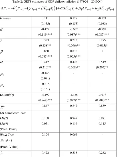
Table 2 shows results when inflation is measured with GDP deflator and these are also

impressive. Unlike Table 1 there is no trace of autocorrelation. Furthermore, the coefficients of the

changes in the lagged inflation and its expected value are insignificant and are dropped from the

[image:7.595.96.507.176.735.2]

estimates in column (2). This made very little change.

Table 2: GETS estimates of GDP deflator inflation (1978Q1 – 2010Q4)







1 1 1



1 1 1 2 2 1

t t

y

t

E

t t

E

t

y

t t

E

t t



 

_



_



_





_

 

_



_



_

  





 

Intercept 0.111

(0.155) 0.128 (0.155) -0.124 (0.083)



-0.477 (0.119)*** -0.602 (0.087)*** -0.592 (0.087)***



0.323 (0.138)** 0.212 (0.096)** 0.175 (0.095)*



0.860 (0.085)*** 0.878 (0.065)*** 1



0.442 (0.210)** 0.425 (0.208)** 0.519 (0.205)** 1



-0.148 (0.091) - - 2



-0.218 (0.151) - -

DUM08Q4 -4.199

(0.969)*** -4.135 (0.977)*** -3.978 (0.984)*** 2

R

0.847 0.842 0.839

LM Serial corr. Test

LM(2) LM(4) (Prob. Value) 0.108 0.051 0.947 0.116 0.971 0.115 Wald Test

0: 1

H  

(Prob. Value)

0.104 0.064 -

(8)

However, the Wald test that  1 holds at a slightly lower level of significance. Estimates

with the constraint that  1are in column (3) and imply that 0.252. This is almost the same as its assumed value in Mankiw and Reis (2003) and close to its estimate of 0.27 in Carroll (2003).

However, estimates of this parameter are more sensitive compared to those in Table 1. These

estimates also imply that the acceleration hypothesis is valid and the long run US Phillips curve is

vertical although 42% to 25% of firms use current information on the expected rate of inflation

efficiently.

4. Conclusions

This paper estimated the SIPC for the USA with an appropriate valid method when both I(1) and

I(0) variables are present in a relationship. Inferences based on our estimates are more reliable than

other estimates with the classical methods. Our estimates imply that the US Phillips curve is vertical

in the long run and between 40% and 25% of firms use information on the expected values

(9)

Data Appendix

Definitions and Data Source: 1978Q1 – 2010Q4

Variable Definition Source

 Percent change from previous quarter at annual rates of Consumer Price Index (seasonally adjusted) or the GDP deflator (seasonally adjusted) and denoted below and in Table 1A as

.

d



Federal Reserve Economic Data (FRED).

1

t t

E_ Forecasts for the CPI Inflation, percent change from previous quarter at annual rates (Seasonally adjusted). The series begins in 1981Q3. For period 1978Q1 – 1981Q2 we use forecasts data of GDP Price Deflator Inflation (the two series in 1980s are very similar).

Survey of Professional Forecaster, Federal Reserve Bank of Philadelphia (SPF).

1

d t t

E_ Forecasts for the GDP deflator Inflation, percent

change from previous quarter at annual rates of CPI (Seasonally adjusted).

SPF

y Real output gap using the Hodrick-Prescott filter

with a smoothing parameter of 1600 (yHP).

Real output gap using linear and quadratic trend (yTR).

FRED

1

t t

E y_ Forecasts for the real GDP (Seasonally adjusted). SPF

DUM06Q4 This dummy is one in this quarter and zero in other periods. It captures the drop (-32% from previous quarter at annual rates) in energy prices caused by a drop in oil prices (-47% from previous quarter at annual rates).

-

DUM08Q4 This is a similar dummy to capture the peak effects of the financial crisis (Lehman Brothers, Merrill Lynch, Fannie Mae, Freddie Mac, etc.).

(10)

[image:10.595.157.439.104.607.2]

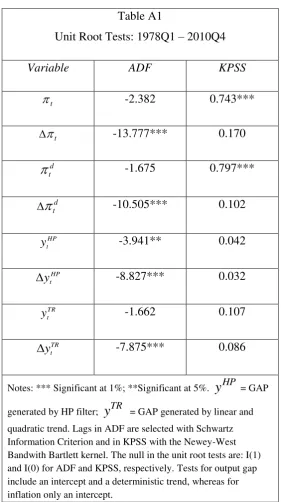
Unit Root Tests

Table A1

Unit Root Tests: 1978Q1 – 2010Q4

Variable ADF KPSS

t

 -2.382 0.743***

t 

 -13.777*** 0.170

d t



-1.675 0.797***

d t



 -10.505*** 0.102

HP t

y -3.941** 0.042

HP t

y

 -8.827*** 0.032

TR t

y -1.662 0.107

TR t

y

 -7.875*** 0.086

Notes: *** Significant at 1%; **Significant at 5%.

y

HP = GAP

(11)

References

Carroll, C. D. (2003) Macroeconomic expectations of households and professional forecasters,

Quarterly Journal of Economics, 118, 269-298.

Khan, H. and Zhu, Z. (2006) Estimates of the sticky-information Phillips Curve for the United

States, Journal of Money, Credit, and Banking, 38, 195-207.

Mankiw, N. G. and Reis, R. (2003) Sticky information: A model of monetary nonneutrality and

structural slumps. In Knowledge, Information and Expectations in Modern Macroeconomics: In

Honour of Edmund S. Phelps, edited by P. Aghion, R. Friedman, J. Stiglitz, and M. Woodford,

Princeton University Press.

Pickering, A. (2004) Sticky information and the Phillips Curve – A tale of two forecasts,

Manuscript, University of Bristol.

Pesaran, H. M., and Shin, Y. (1999) Autoregressive distributed lag modelling approach to

cointegration analysis, Chapter 11, in: Storm, S. (ed.), Econometrics and Economic Theory in the

20th Century: The Ragnar Frisch Centennial Symposium, Cambridge University Press.

Rao, B. B. (2007) Estimating short and long-run relationships: a guide for the applied economist,