Family dissolution and precautionary savings: an empirical analysis

Munich Personal RePEc Archive

Family dissolution and precautionary

savings: an empirical analysis

Pericoli, Filippo Maria and Ventura, Luigi

May 2011

Family dissolution and precautionary savings: an empirical analysis

Filippo Pericoli! and Luigi Ventura"12

May 2011

Abstract

The main research question of this paper is whether or not the risk of family disruption has an impact on the consumption/saving decisions of households. Although little empirical work exists in this area, often presenting indirect evidence, the theory is divided over the effect of family risk over saving and wealth accumulation. By using data from the Italian Survey on Households Income and Wealth, we build a probabilistic model to assess the probability of marital splitting, and then we insert this probability as a distinct or interacted regressor, in a statistically consistent way, into a linear model of consumption. Furthermore, we study the differential behaviour, in terms of consumption/saving choices, of couples experiencing marital splitting over the subsequent two years. The main result of our analysis is that family disruption risk generates precautionary savings, reducing current consumption. In fact, according to our estimates, on average, the risk of divorce generates an amount of additional yearly precautionary savings of around 800 euros at constant prices of the year 2000, which represents 11% of overall household savings.

! Italy’s Ministry of Economy and Finance, Rome, University Tor Vergata, Rome.

" Sapienza, University of Rome

1 _{Corresponding author: Luigi Ventura, Dipartimento di Economia, Circonvallazione Tiburtina, 4, 00185 Roma;} email: luigi.ventura@uniroma1.it

2

1. Introduction

Since the seminal work by Leland (1968) the precautionary motive for saving has been the object of intense research activity.

The precautionary motive for saving can be multi-faceted. In fact, a recent paper by Kennickell and Lusardi (2005) explored several sources of risk that generate a precautionary saving motive. This includes income risk, health risk, business risk and liquidity constraints. By using a subjective measure of desired precautionary savings derived from the 1995 and 1998 Survey of Consumer Finance as dependent variable, they showed that besides earnings risk, which is usually the focus of the empirical literature, most other sources of risk are also relevant.

Precautionary saving is closely intertwined with opportunities for risk sharing. Some authors (see, for example, Devereux and Smith (1994)) suggest that more risk sharing opportunities may translate into less saving, as there are better ways of dealing with the effects of uncertainty.

The idea that marriage provides some sort of risk sharing among its members is well known. Ever since Becker's contributions (1973, 1974), households economics has often highlighted the idea that marriage engenders risk sharing among a couple. The basic idea is that transfers between spouses help smooth out a certain amount of variability in individual income streams. It might even be conceivable, as in Chami and Hess, (2005), that individuals also choose to marry in order to hedge against macroeconomic risks. A fairly large set of applied studies (most commonly using micro data) show that risk sharing does seem to occur within marriages (this is the case, for example, of the works by Rosenzweig and Wolpin, 1985, 1994; Rosenzweig, 1988; Rosenzweig and Stark, 1989, among the others).

If marriage features, as a fundamental ingredient, a certain amount of trust and information, it may also help reduce problems of moral hazard, adverse selection, and deception (as underscored by Kotlikoff and Spivak, 1981) thereby impacting insurance markets. Moreover, transaction costs in marriage may be lower than those associated with formal insurance and financial instruments. As an insurance instrument, therefore, marriage would be particularly efficient.

On the other hand, to the best of our knowledge, most stylized models of saving do not explicitly account for life-changing events such as marriage and divorce, which may have sizeable and long-lasting implications on income and consumption patterns.

For example, Lupton and Smith (2003) remark that “very little theoretical or empirical work has addressed this issue” (i.e. that of a link between marriage and saving).

Also, as is shown in this paper, the consequences of the disruption of the family arrangement (i.e. the collapse of marriage), are far from clear from a consumption/saving standpoint.

Even those few who deal with this problem do not reach unambiguous (theoretical) conclusions, at least as far as the effects of divorce risk on saving are concerned.

In fact, opposing forces may be at work: on the one hand, divorce is costly (legal fees, etc...), and leads to a potentially very large loss of economies of scale linked to marriage. This may be perceived as a negative shock, which might bring about an increase in precautionary saving. On the other hand, in the presence of divorce prospects saving becomes riskier, as the resulting assets must be split among the couple, leading to a decrease in saving; moreover, divorce, or the risk thereof, may also decrease the return to saving for the couple, in the presence of costs cutting into the net worth of the couple, or in the presence of remarriage, thus diminishing the incentives to save.

risk upon consumption/saving choices, mostly using an indirect approach. For example, Gonzalez-Ozcan (2008) present indirect evidence about the impact of divorce risk upon saving in the household, by considering the legalization of divorce in Ireland in 1996 as an exogenous increase in the likelihood of marital dissolution. They do find a positive relationship, resorting to a difference in difference estimation (though, we believe, with some problems in properly defining the control and treatment groups).

A remarkable contribution to this literature is the work by Pierce and Finke (2006). By identifying households that will divorce over a 5 year period in the Panel Study of Income Dynamics (1994-1999), they show that divorce prone households save significantly more than couples remaining married, in the years before the actual occurrence of divorce.

More recently, Voena (2010) proposed a model to assess the impact of different property rights regimes among spouses over the accumulation of assets in the household and the supply of labor then tests the model by using US data. Interestingly, one of the indications of the paper is that when the probability of divorce increases and assets are equally split among spouses, men tend to increase savings (and asset accumulation), to offset the possible loss of half of their assets to wives if divorce comes about.

Our paper explores the consequences of family dissolution risk onto consumption and (precautionary) saving, by using a very simple theoretical model, and by estimating an empirical model that explicitly combines an estimation of marital dissolution risk with one of consumption/saving. By doing so, we contribute to the rather thin body of literature dealing with a problem that has become increasingly important, as family instability has become more prevalent. The rest of the paper is organized as follows: in paragraph 2 we propose a theoretical model describing consumption/savings choices for a married couple exposed to risk of marital dissolution; in paragraph 3 we report the results of our empirical analysis on a panel of Italian households. By means of a two-stage methodology, we find that the risk of divorce reduces nondurable consumption and generates precautionary savings, with an intensity depending on household income.

2. A simple model of divorce risk and precautionary savings

2.1. The institutional framework

Before we introduce our simple theoretical model, it is useful to describe at some length the underlying institutional set-up, which is also the reference framework for the ensuing empirical analysis. This concerns the time horizon 1989-2006, which was characterized by a substantial stability in the set of norms regulating divorce in Italy. Indeed, divorce was introduced in Italy in 1970 by a law that has registered only minor changes since.

and possibly the children a lifestyle comparable to that experienced during the marriage. The stock of wealth owned by an individual at the time of the marriage, as well as heritages and gifts received during the marriage are always excluded from the stock of wealth eventually shared with the partner at the time of divorce. However, savings and durable goods accumulated during the marriage must be split equally between the husband and the wife in case of divorce, but the spouses can opt, at the time of marriage or even later, for an alternative “disjoint” regime, where savings and durable goods accumulated during the marriage are not shared with the wife/husband3.

To sum up, within the Italian legal framework a relevant fraction of individual wealth (the rental income potentially obtainable from the house and/or significant fractions of current and future wages for wife/husband and children alimony) must be split between the husband and the wife at the moment of divorce, but at the same time a large fraction of individual wealth may remain potentially untouched by the economic agreement approved by a judge (the stock of wealth at the time of marriage, heritages, gifts, second houses and in most cases also personal savings and durables acquired within the marriage).

As a consequence, in the Italian case it is not possible to determine a priori that consumption/savings choices result from an individual, rather than a unitary or a collective decision process, as the appropriateness of a particular model will depend on the type of household under analysis and, in particular, on the spouses’ initial endowments. Roughly speaking, one may conjecture that low-income and liquidity constrained couples cannot resort to precautionary savings to improve on the intertemporal distribution of consumption. On the other hand for middle-income couples, who generally share the ownership or the use of a unique house, the amount of wealth to be split at the moment of the legal separation represents a very high share of their permanent income, and therefore the collective choice model seems to be appropriate to describe consumption/savings choices. Lastly, for high-income or wealthy individuals the amount of resources to be split at the moment of divorce represents a marginal fraction of their permanent income, and therefore the individual model with partial sharing of resources seems the best to describe consumption/saving choices.

2.2 A model of partial income pooling with heterogeneous preferences.

When one tries to model household’s saving, one is faced with a fairly important challenge: should household decisions be analysed in the framework of a unitary model, in which the household behaves as if it was endowed with its own objective function and in which there is only one household income constraint, or with a model that recognizes that individual members of the household have their own utility functions and/or their own income constraints? An example of the latter applied to the analysis of saving decisions is Nordblom (2004). Consumption decisions of individuals in couples have been modelled as individual decisions e.g. by McElroy and Horney (1981) and Browning et al. (1994), and so have labor supply decisions (e.g. by Grossbard-Shechtman (1984) and Chiappori (1988a, 1988b)).

In collective models, where household preferences are a convex combination of the spouses’ utility function, the analysis of each partner’s preferences also becomes relevant, in terms of overall

3

consumption and saving behaviour, investment, and other choice variables. In fact, there exists a rich literature on gender differences in saving behavior which explores how different attitudes toward risk and time as well as different socio-economic situations impact consumption/saving decisions. This has been mostly analyzed in the context of developed countries (see, among the others, Bajtelsmit and Bernasek (1996) and Floro and Seguino (2002, 2003), for a survey of empirical works and some theoretical modelling of this issue).

Our approach, in what follows, is based on a somehow eclectic approach. We will present a model that we name “partial income pooling with heterogeneous preferences”, where the spouses independently decide over the allocation of their own income between consumption and saving, but also pool a fraction of their income, where half of the pooled income enters into each individual’s total income. This model does not belong to either the class of unitary preference models, nor to one of collective preference models. As it can encompass both partial and complete risk pooling, it can accommodate both cohabiting and married couples, and is quite similar to a model recently published by Nordblom (2004).

The main research question of the model is to investigate the difference in consumption and saving between a couple that is not subject to marriage dissolution risk and a couple that is subject to marriage dissolution risk, rather than on the difference in consumption between a couple, subject or not to marriage dissolution risk, and two single individuals. Moreover, we will assume that the only decision makers in the household are the spouses, and that one of them will be dominant, as the primary earner, who will have to contribute some amount of money to other spouse, in case of divorce.

Agents live for two periods, the second being affected by some income uncertainty, represented by two possible realizations of income, denoted by y_l (y low) and y_h (y high).

We can therefore recognize four possible states of the world: both F and M have a low income, F gets a low income and M a high income, F gets a high income and M a low income, both

F and M get a high income. The corresponding probabilities will be denoted by !₁,

!

!

!

!

!

3 1

and

!

!

!

! , then the income risks of the two individuals would be

perfectly correlated, but of course this need not be the case, in general.

Agents can save an amount S of their income at period 1, to buffer against income uncertainty in the second period. For simplicity, we also assume that the effects of time preference and interest rate cancel out.

The aim of the model is to show that, under plausible assumptions, marital disruption risk increases precautionary saving, which is what we also find out empirically from our data analysis. As we are not specifying a particular utility function for the decision makers in the household, the results will hold regardless of rates of time preference, degree of risk aversion, and other individual specific features.

In our model both decision makers in the couple make a decision as to the extent of saving.

Each decision maker (i and j) pools in both periods a fraction !iof his/her income, keeping the rest

separate. Half of the pooled income will add to the un-pooled component of each spouse’s income.

We will assume that the parameters !i and !j, as well as the parameters!i

' _!

j

'_{defined in the}

endogenously. In the models by Grossbard-Shechtman and Neuman (1988) and Chiappori (1988a, 1988b) the fraction of income shared depends on marriage market forces and distribution factors (Becker (1973) and Browning et al. (1994).

Each decision maker i has preferences represented by the generic instantaneous utility function (.)

i

u _{, accommodating all possible time preference rates and risk attitudes. Following Leland (1968)}

we will assume that the third order derivative of the utility functions be positive to have a positive precautionary motive. In case of marital splitting (with probability_{! >}0_{), the dominant spouse (i}

in the sequel) will continue to pool a fraction !i

'_<!

i which will be added to the other spouse’s income (this should capture alimony or other kind of transfers); the latter will, in addition, incur a cost of marital disruption, c.

The problem of agent i, denoting by ! !0_{the probability of marital splitting, will be that of:}

)), ) ' 1 (( ) 1 ( ) ) ' 1 (( ( )) 2 ) 1 (( ) 2 ) 1 (( ) 2 ) 1 (( ) 2 ) 1 (( )( 1 ( ) 2 ) 1 (( 4 3 2 1 1 1 1 S y u S y u S y y y u S y y y u S y y y u S y y y u S y y y u U Max hi i i li i i hj j hi i hi i i lj j hi i hi i i hj j li i li i i lj j li i li i i j j i i i i i i S + ! ! + + + ! + + + + ! + + + + + ! + + + + ! + + + + + ! ! + ! + + ! = " # " # $ " " " # " " " # " " " # " " " # $ " " " (1)

with first order condition:

)). ) ' 1 (( ' ) 1 ( ) ) ' 1 (( ' ( )) 2 ) 1 (( ' ) 2 ) 1 (( ' ) 2 ) 1 (( ' ) 2 ) 1 (( ' )( 1 ( ) 2 ) 1 (( ' 4 3 2 1 1 1 1 S y u S y u S y y y u S y y y u S y y y u S y y y u S y y y u hi i i li i i hj j hi i hi i i lj j hi i hi i i hj j li i li i i lj j li i li i i j j i i i i i + ! ! + + + ! + + + + ! + + + + + ! + + + + ! + + + + + ! ! = ! + + ! " # " # $ " " " # " " " # " " " # " " " # $ " " " (2)

Let us now consider the maximization problem of the other, non-dominant member of the household. The problem of agent j, denoting by !!0_{the probability of marital splitting, will be}

that of: )), ( ) (( ) (( ) (( ( )) 2 ) 1 (( ) 2 ) 1 (( ) 2 ) 1 (( ) 2 ) 1 (( )( 1 ( ) 2 ) 1 (( ' 4 ' 2 ' 3 ' 1 4 2 3 1 1 1 1 S c y y u S c y y u S c y y u S c y y u S y y y u S y y y u S y y y u S y y y u S y y y u U Max hi i hj j li i hj j hi i lj j li i lj j hi i hj j hj j j li i hj j hj j j hi i lj i lj j j li i lj j lj i j i i j j j j j j S + ! + + + ! + + + ! + + + + ! + + + + + ! + + + + ! + + + + ! + + + + + ! ! + ! + + ! = " # " # " # " # $ " " " # " " " # " " " # " " " # $ " " " (3)

)). ( ' ) (( ' ) (( ' ) (( ' ( )) 2 ) 1 (( ' ) 2 ) 1 (( ' ) 2 ) 1 (( ' ) 2 ) 1 (( ' )( 1 ( ) 2 ) 1 (( ' ' 4 ' 2 ' 3 ' 1 4 2 3 1 1 1 1 S c y y u S c y y u S c y y u S c y y u S y y y u S y y y u S y y y u S y y y u S y y y u hi i hj j li i hj j hi i lj j li i lj j hi i hj j hj j j li i hj j hj j j hi i lj i lj j j li i lj ji lj j j i i j j j j j + ! + + + ! + + + ! + + + + ! + + + + + ! + + + + ! + + + + ! + + + + + ! ! = ! + + ! " # " # " # " # $ " " " # " " " # " " " # " " " # $ " " " (4)

Proposition 1. Under the conditions

(

)

y y hi i j i i j j j li i i lj j li i ! + > + + ! > " " # $ % % & ' + _' 1 1 1 1 ' 2 , 2 ( ( ( ( ( ( (

, and for a sufficiently large

probability of getting a low income, !, divorce risk will induce both members of a couple into more precautionary savings.

Proof. To show that S is higher when the couple faces some divorce risk, we have to show that the r.hs. in (2) and (4) are larger when !>0_{than when !=}0_{, if S is the same. To check this, let us}

rewrite the right hand sides of (2) and (4) when !=0 _as:

))). 2 ) 1 (( ' ( 1 )) 2 ) 1 (( ' ( 1 )( 1 ( ))) 2 ) 1 (( ' ( )) 2 ) 1 (( ' ( ( 4 3 2 1 S y y y u S y y y u S y y y u S y y y u hj j hi i hi i i lj j hi i hi i i hj j li i li i i lj j li i li i i + + + ! ! + + + + ! ! ! + + + + ! + + + + ! " " " # # " " " # # # " " " # # " " " # # # (5) and: ))). 2 ) 1 (( ' ( 1 )) 2 ) 1 (( ' ( 1 )( 1 ( ))) 2 ) 1 (( ' ( )) 2 ) 1 (( ' ( ( 4 3 2 1 S y y y u S y y y u S y y y u S y y y u hi i hj j hj j j li i hj j hj j j hi i lj j lj j j li i lj j lj j j + + + ! ! + + + + ! ! ! + + + + ! + + + + ! " " " # # " " " # # # " " " # # " " " # # # (6)

This can be represented graphically as shown in Figure 1a, where the right hand side of (2) in the case !=0 _{can be geometrically interpreted as a point X on the chord AB, where the points A}

and B, respectively, lie on the chords CD and EF. For simplicity, we set:

S y y

y

y = ! _{i li} + i li + j lj +

2 ) 1 ( 1 " " " , , 2 ) 1 ( 2 S y y y

B C

E D

, 2

) 1 (

3 S

y y

y

y = !"_{i hi} +"i hi +"j lj +

, 2

) 1 (

4 S

y y

y

y = !"_{i hi} +"i hi +"j hj +

Figure 1a. The geometry of proposition 1

y₁' y₁ y₂ y3 ' 4

y y₄

with

, )

' 1 (

'

1 y S

y = !"_{i li} +

. )

' 1 (

'

4 y S

y = !"_{i hi} +

On the other hand, condition (2) in the case !>0 _{contains, in its right hand side, a convex}

combination of the r.h.s. of (2) with an additional term, with weights (1"!) and !, respectively.

The latter is also a convex combination, and can be represented as the segment GH.

The condition i yli jylj

(

)

2 ! !

! !

" > # # $ % &

& '

( +

insures that y₁' < y₁, and consequently that the

point G lies on the left of the point C. Point H could be on either side of F, as y₄' y₄ < >

. However, if

!is sufficiently large, point X~will lie above AB. Any convex combination of X and X~will therefore entail a level of marginal utility larger than X. To restore equality between the lhs and the rhs of (4), S must increase, i.e. precautionary saving must be higher.

Similarly, we can show the same result for the other, j, spouse. In this case, condition (4) in F

G

H

X X~

A U’

the case !>0_{can be written as:} ))). ( ' 1 ) (( ' 1 )( 1 ( )) (( ' ) (( ' ( ( ))) 2 ) 1 (( ' 1 ) 2 ) 1 (( ' 1 )( 1 ( )) 2 ) 1 (( ' ) 2 ) 1 (( ' ( )( 1 ( ) 2 ) 1 (( ' ' 4 ' 2 ' 3 ' 1 4 2 3 1 1 1 1 S c y y u S c y y u S c y y u S c y y u S y y y u S y y y u S y y y u S y y y u S y y y u hi i hj j li i hj j hi i lj j li i lj j hi i hj j hj j j li i hj j hj j j hi i lj i lj j j li i lj ji lj j j i i j j j j j + ! + ! + + ! + ! ! + + ! + + + + ! + + + + + ! ! + + + + ! ! ! + + + + ! + + + + + ! ! = ! + + ! " # # " # # # " # # " # # # $ " " " # # " " " # # # " " " # # " " " # # # $ " " " (4’)

Setting, for simplicity:

S y y

y

y = ! _{j lj} + i li + j lj +

2 ) 1 ( 1 " " " , 2 ) 1 ( 2 S y y y

y = !"_{j lj} +"i hi +"j lj +

, 2 ) 1 ( 3 S y y y

y = !"_{j hj} +"i li +"j hj +

, 2 ) 1 ( 4 S y y y

y = !"_{i hi} +"i hi +"j hj +

, '

'

1 y y c S

y = _lj +"_{i li} ! +

, '

''

1 y y c S

y = _lj +"_{i hi} ! +

S c y y

y₄'' = _hi +"_i' _li ! +

.

' '

4 y y c S

y = _hi +"_{i hi} ! +

The new situation, in terms of marginal utilities, is now represented in Figure 1b.

The condition y_1j + jy1j + iy1i > y_1j + _i'y_hi !c

2 "

" "

insures that point G lies to the left of point

C. The same argument used for individual i can also be used to show that pointX~will lie above point X, if !is sufficiently large.

The conditions i yli jylj >

(

)

" " # $ % % & ' + _' 1 1 1 1 ' 2 , 2 ( ( ( ( ( ( (

are more

likely to hold, the higher the share of income pooled by spouse i following divorce, the more similar the shares of income contributed by the spouses in marriage, and the more similar the levels of income. The second condition is more likely to hold for a relatively heavier cost of divorce for the weaker spouse.

Assuming that income sharing in the couple is endogenously determined would not radically alter the results of our analysis, in as much as we impose the constraints that some sharing does

occur within marriage, and that !i'_<!

B C

E D

between two singles and a married couple (which would be strongly influenced by the income sharing process within the couple), but rather in comparing the savings of a couple not affected by divorce risk with those of a couple more or less affected by such risks.

Figure 1b. The geometry of proposition 1

y₁'' y₁' y₁ y₂ y3 '' 4

y y'₄ y₄

3. Marital dissolution and precautionary savings: an empirical analysis.

3.1. The empirical strategy

To evaluate the empirical relevance of precautionary saving behaviour originated by the risk of divorce we will follow a methodology similar to the one recently used to assess the influence of unemployment risk on consumption choices within a micro-econometric framework (De Lucia and Meacci (2005), Benito (2006)), based on a two-step approach. The first stage consists in the estimation of a probabilistic model for generating a proxy for the risk of divorce, while in the second stage this generated risk variable is introduced as an additional regressor in a standard consumption or saving model.

Applying this methodology to the analysis of precautionary savings generated from the risk of divorce presents a peculiar difficulty, originating from the fact that marital dissolution modifies the family’s structure, which affects the level of consumption in a complex way due to the departure of at least one person from the household. This event makes it impossible to disentangle the effects on (precautionary) savings originated from the risk of divorce from the effects on savings linked to the change in the family’s composition. Another difficulty arises from the fact that estimating a binary model in the first stage for contemporaneous marital status by employing contemporaneous

socio-F G

H

X X~

A U’

demographic and economic variables is quite problematic, as these variables are, at least up to some extent, both a consequence and a cause of the marital separation. Thus, the estimated parameters would be affected by an endogeneity bias originated by simultaneity. To overcome this difficulty we resort to estimating a probabilistic model where our dependent binary variable represents, instead of the actual marital status, the future marital status, (in two years time). A probit model for future marital status has been estimated out of a set of socio-demographic and economic variables one period (two years) before the possible occurrence of divorce. After identifying the main determinants of marital dissolution, we assign each household an estimate of the corresponding probability of divorce. In the second stage of the analysis this generated regressor is added to the set of explanatory variables in a rather standard consumption model to assess the impact of divorce risk on household consumption choices.

3.2. The dataset

The empirical exercise is based on the Bank of Italy’s Survey on Household Income and Wealth (SHIW thereafter), a sample survey representative of the Italian population. The survey started in year 1965 and from year 1987 it has been conducted every two years, with the only exception being the 1998 wave, carried out three year after the 1995 one. In the period covered by our empirical analysis, each wave of the survey contains detailed statistics over around 8,000 households. Since 1989 the survey includes a panel subsample whose weight has significantly increased over time, representing 14,6% of the interviewed households in year 1989 to a maximum of 50,1% of the sample size in year 2006 (Jappelli and Pistaferri 2010). The SHIW survey is a rotating split panel, where at each wave the sample consists of a subsample of panel households chosen among households interviewed in the preceding wave, and a subsample of cross-section households, entering the sample for the first time. In years 1991 and 1993 the panel component has been chosen on the basis of the willingness of the family, previously expressed, towards being interviewed once again, while since 1995 the panel subsample has been randomly chosen within the cross-section component of the previous wave; this change is likely to have increased the quality of the sample survey, by mitigating the bias induced by self-selection of households into the panel (Giraldo, Rettore and Trivellato, 2001).

The survey reports values for the main social and demographic variables for each member of the household such as age, marital status, professional condition, and many others. It also reports, aggregated at household level, data on income and savings, as well detailed data on real and financial wealth. By any account, this is the most frequently used dataset for carrying out micro-econometric research in the field of consumption and saving behaviour in Italy.

the same procedure would have been reiterated one more time, to the previous wave (and so on, till the first wave). If the individual was married in the previous survey then this observation would have constituted one “divorce in two year’s time” couple, and entered into our final sample. Using this method we selected all households experiencing divorce in the course of their survey participation. Unfortunately, the total number of such households is very limited, as it seems that, even if only on logistic grounds (relocation of one partner, little willingness to keep on participating in the survey, etc…) couples experiencing divorce while they are part of our panel very often discontinued participation. The rest of our sample (actually, the vast majority of it) is made of married couples remaining such in all surveys they take part in.

These criteria led us to identify a dataset including a total of 8,028 distinct households, with only 165 occurrences of divorce/separation, while the remaining 7,863 couples remain married. Data on consumption, savings, wealth as well as all the monetary variables have been deflated to their year 2000 values by using the gross domestic product deflator. In table 1 we report the main statistics over this selected sample for the whole sample and separately for stable and “close to marital split” couples. From the available statistics it turns out that divorce-prone households are generally held by a younger and more educated spouses and by a wife with a higher probability of participating in the labour force.

[Table 1]

We can also observe that average total consumption is larger for “risky” couples, whereas total wealth is smaller. Other socio-demographic variables (e.g. number of household components and number of income earners are quite similar across both groups).

3.3. Empirical results

In the first stage of the empirical analysis we estimated a probit model where the dependent variable is equal to 1 if the married couple will be divorced/separated after two years and is equal to 0 otherwise.

[Table 2]

assumption of exogeneity over the dummy variable which is equal to 1 if the women earns more than a certain threshold (10,000 euros at constant prices of year 2000) and is equal to 0 otherwise. To do so, we have implemented the procedure by Rivers and Vuong (1988), as suggested by Wooldrige (2002).

In more detail, we regressed our potentially endogenous variable on all the remaining exogenous variables on the right hand side of the equation plus the number of years of education of the wife, a variable which is strongly significant in this auxiliary regression but scarcely so in the probit model. We then included the residuals of this auxiliary regression in the probit model and estimated a statistically insignificant coefficient (with a p-value equal to 0.6); this suggests that we cannot reject the hypothesis of exogeneity. As an additional robustness check we have estimated the simultaneous bivariate probit (with dependent variables “the couple will divorce within two years” and “the wife earns at least than 10,000 euros at constant prices of year 2000”) by maximum likelihood and again we have found that the correlation between the residuals in the two equation is not significantly different from zero (with a p-value equal to 0.7), as shown in table 3

[Table 3]

In order to assess the classificatory performance of our model we have chosen as cut-off point the average incidence of divorce observed in the sample, which is around 2 percentage points. The results obtained (reported in table 4) indicate that our model classifies correctly around two thirds of the observations. The major shortcoming of the estimated model consists in the fact that it often predicts divorce when it actually does not occur in our dataset, most likely because we do not observe the entire history of marriages, but only a short fraction of that; this is also reflected in the fact that over a longer time span the probability of divorce is higher than the one observed in our dataset. Indeed, according to statistics released by the Italian National Statistical Institute (ISTAT), in 2005 the average occurrence of marital separation (including divorce) reached the value of 27% within the overall number of marriages.

[Table 4]

[Table 5]

Lastly, nondurable consumption depends negatively on whether or not the wife is working, whether the wife is self employed, whether the husband is self-employed and lastly, on the wife and husband’s educational attainments.

In many ways we can see that the consumption model is identified. First and foremost, many of the regressors included in the first stage Probit model (namely the age of wife, the squared age difference between the spouses, the presence of children aged less than five, the working status of the husband, the wife earnings dummy) do not display statistically significant coefficients when included in the consumption equation (results not reported, but available on request). Secondly, our risk variable does not enter the consumption model as such, but interacted with income, which would greatly reduce a hypothetical identification problem. Lastly, the first stage estimation is non linear, which also greatly reduces the extent of an identification problem, even if the variables included in both equations (the non linear and the linear one) were exactly the same (see Wooldrige, 2002).

A similar analysis has been conducted for durable savings, but we did not find any significant effect of divorce risk. Conversely, we did find a positive effect of divorce risk on overall household savings, as can be seen from the following table, supporting the theoretical prediction that the higher the risk of divorce, the higher the extent of savings.

[Table 6]

As shown in table 7, the interacted variable, i.e. the risk of divorce times income, would be responsible, on average, for around 800 euros of savings, which accounts for about 11% of mean overall savings.

[Table 7]

In the spirit of Pierce and Finke (2006) we have also performed a different exercise, consisting of the following steps:

1) rather than estimating the probability of marital disruption for each household of the sample, instead we directly included in our analysis a dummy variable equal to 0 if the married couple will be still married after two years and equal to 1 if the married couple will experience marital disruption within the following two years (this is actually the same variable as the one on the left hand side of the probit model reported in the preceding pages).

case.

[Table 8]

3) Lastly, a log-linear regression model for non durable consumption has been run by using this dummy variable, instead of the probability of marital splitting, as in the previous consumption equation. This way, we could analyze the differential behaviour in consumption of households actually running into a marital splitting in the following two years, as opposed to households remaining stable over the same horizon.

The results of this analysis are summarized in Table 9; the estimates (weakly) support the view that future marital disruption positively affects the level of consumption, but the interaction between the logarithm of income and the divorce variable negatively affects the logarithm of nondurable consumption, implying that households experiencing marital disruption within a fairly short horizon feature a lower elasticity of consumption over labour income, together with a higher level of autonomous consumption. The overall (differential) effect upon saving will therefore depend on the level of income.

[Table 9]

4. Concluding remarks

The empirical findings presented in this paper point to an important role played by marital disruption risk in generating more precautionary savings. This has been rationalized by means of a simplified theoretical model, showing that an increase in the objective probability of marital disruption has an indeterminate effect on household consumption and (precautionary) savings.

Our empirical analysis points at an increase in (precautionary) savings for those couples more likely to experience family distress. This appears to be true for non durable consumption, while we did not find any similar effect on durable consumption.

References

Bajtelsmit, V.L. and Bernasek, A. (1996), “Why Do Women Invest Differently Than Men?”, Financial

Counseling and Planning, 7, 1-10.

Becker, G.B.(1973). “A Theory of Marriage: Part I”, The Journal of Political Economy,81, 813-846.

Becker, G.B. (1974). “A Theory of Marriage: Part II”, The Journal of Political Economy,82, 11-26.

Benito, A. (2006). “Does Job Insecurity affect Household Consumption?”, Oxford Economic Papers, 58, 157-181.

Browning, M., Bourguignon, F., Chiappori, P.A., Lechene, V. (1994). “Income and Outcomes: a Structural Model of Intrahousehold Allocation”, Journal of Political Economy, 102(6), 1067-1096.

Chami, R., Hess, G. (2005). “For Better or For Worse? State-Level Marital Formation and Risk Sharing”,

Review of Economics of the Household, 3(4), 367-385.

Chiappori, P.A. (1988a). “Rational Household Labor Supply”, Econometrica, 56, 63-89.

Chiappori, P.A. (1988b). “Collective Labor Supply and Welfare”, Journal of Political Economy, 100, 437-467.

De Lucia, C., Meacci, M. (2005). “Does Job Security Matter for Consumption? An Analysis on Italian Microdata”. Istituto di Studi e Analisi Economica, Working Paper,54.

Devereux, M.B. and Smith, G.W. (1994). “International Risk Sharing and Economic Growth”,

International Economic Review, 35, 3.

Eisenhauer, J. and L. Ventura, (2005), "The Relevance of Precautionary Saving", German Economic

Review, 6, 2005.

Floro, M.S. and S. Seguino, (2002), “Gender Effects on Aggregate Saving”, Working Paper Series n. 23, World Bank.

Floro, M.S. and Seguino, S.(2003). “Does Gender Have Any Effect on Aggregate Saving? An Empirical Analysis”, International Review of Applied Economics, 17(2), 147-166.

Giraldo, A., Rettore, E., Trivellato, U.(2001). “Attrition Bias in the Bank of Ital’s Survey of Household Income and Wealth”, Proceedings of the International Conference on Quality in Official Statistics,

Stockholm, May 14-15, 2001.

Gonzalez, L., Ozcan, B. (2008). “The Risk of Divorce and Household Saving Behavior”, IZA Discussion

Papers, n° 3726.

Greene, W. H., (2003). “Econometric Analysis”, Prentice Hall, New Jersey.

Grossbard-Shechtman, S.A. (1984). “A Theory of Allocation of Time in Markets for Labor and Marriage”, Economic Journal, 94(4), 863-882.

Grossbard-Shechtman, S.A., Neuman, S. (1988). “Woman’s Labor Supply and Marital Choice”, Journal

of Political Economy, 96(6), 1294-1302.

Jappelli, T., Pistaferri, L. (2010). “Does Consumption Inequality Track Income Inequality in Italy”,

Review of Economic Dynamics, 13(1), 133-135.

76(3), 455-469.

Kennickell, A. and Lusardi, A. (2005). “Disentangling the importance of the precautionary saving motive”, Working paper, Dartmouth College.

Kotlikoff, L.J., Spivak, A. (1981). “The Family as an Incomplete Annuities Market”, Journal of Political

Economy, 89, 372-391.

Leland, H.E. (1968). “Saving and Uncertainty: The Precautionary Demand for Saving”, The Quarterly Journal of Economics, 82, 465-473.

Lupton, J. P., Smith, J. P.(2003). “Marriage, Assets and Savings”, in Marriage and the Economy: Theory

and Evidence from Advanced Industrial Societies, Shoshana A. Grossbard-Shechtman Ed.

Cambridge: Cambridge University Press.

Maddala, G. S., (1983). “Limited-Dependent and Qualitative Variables in Econometrics”, Cambridge University Press, Cambridge.

McElroy, M.B., Horney, M.J. (1981). "Nash-Bargained Household Decisions: Toward a Generalization of the Theory of Demand", International Economic Review 22(2), 333-349.

Murphy, K. M., Topel, R. H. (1985). “Estimation and Inference in Two-Step Econometric Models”,

Journal of Business and Economics Statistics, 3, 88-97.

Nordblom, K. (2004). “Cohabitation and Marriage in a Risky World”, Review of Economics of the

Household, 2(3), 325-340.

Pierce, N. L., Finke, M.S. (2006). “Precautionary Savings Behavior of Maritally Stressed Couples”,

Family and Consumer Science Research Journal, 34, 223-240.

Rivers, D., Vuong, Q.H.(1988). “Limited Information Estimators and Exogeneity Tests for Simultaneous Probit Models”, Journal of Econometrics, 39, 347-366.

Rosenzweig, M. R. (1988). “Risk, Implicit Contracts and the Family in Rural Areas of Low-Income Countries”, Economic Journal, 98, 1148-1170.

Rosenzweig, M. R.., Stark, O. (1989). “Consumption Smoothing, Migration, and Marriage: Evidence from Rural India”, Journal of Political Economy, 97, 905-926.

Rosenzweig M. R., Wolpin, K. I. (1985). “Specific Experience, Household Structure and Intergenerational Transfers: Farm Family Land and Labor Arrangements in Developing Countries”,

Quarterly Journal of Economics, 100, 961-987.

Rosenzweig M. R., Wolpin, K. I. (1994). “Parental and Public Transfers to Young Women and their Children”, American Economic Review, 84, 1195-1212.

Voena, A. (2010), “Yours, Mine and Ours: do Divorce Laws Affect the Intertemporal Behaviour of Married Couples?”, Job Market Paper.

Table 1. Main statistics for married couples in the selected sample, years 1989-2006 (average values, when not otherwise specified)

Married couples

Married couples which are still married after two

years

Married couples which are separated/divorced

after two years

Resident in North 39.7% 39.5% 45.5%

Resident in the Middle 20.6% 20.5% 24.8%

Resident in the South or Islands 39.7% 40.0% 29.7%

No. of household components 3.4 3.4 3.4

No. of children 1.3 1.3 1.3

No. of income earners 1.9 1.9 1.8

Age of the husband 53.6 53.8 45.1

Age of the wife 49.9 50.1 41.6

Educational attainment of the husband (1-6) 3.1 3.1 3.3

Educational attainment of the wife (1-6) 2.9 2.9 3.3

The husband works as employee 42.9% 42.8% 50.3%

The husband works as self-employed 17.3% 17.1% 26.7%

The husband is retired or out of the labour force 39.7% 40.1% 23.0%

The wife works as employee 25.6% 25.2% 45.5%

The wife works as self-employed 6.7% 6.7% 6.7%

The wife is retired or out of the labour force 67.7% 68.1% 47.9%

Propensity to consume (median value) 0.78 0.78 0.80

Household income 30,010 29,991 30,878

Total consumption 21,908 21,874 23,569

Nondurable monetary consumption 14,872 14,858 15,530

Durable consumption 1,881 1,867 2,558

Savings 7,368 7,378 6,890

Net wealth 192,397 192,828 171,852

Net wealth in the house where the family lives 108,849 109,018 100,798

Number of observations 8,028 7,863 165

Table 2. Probit analysis – Dependent variable: the couple will divorce within two years

Independent variables Coefficients Marginal effects

Age of the wife -0.029***

0.004

-0.001*** 0.000

Squared age difference between husband and wife 0.001** 0.000

0.000** 0.000

Presence of at least one child aged less than five -0.231*** 0.081

-0.008*** 0.003

The husband works as employee -0.190** 0.074

-0.007** 0.003

The wife earns at least 10,000 euros per year 0.278*** 0.070

0.011*** 0.003

Time trend 0.146***

0.029

0.005*** 0.001

Time trend squared -0.009*** 0.002

-0.000*** 0.000

Constant -1.115***

0.207

Number of observations 8,028

Pseudo R-squared 0.085

Table 3. Biprobit analysis – Dependent variables: “the couple will divorce within two years” and “the wife earns at least than 10,000 euros at constant prices of year 2000”

Independent variables\Dependent Variables The couple will divorce within two years

The wife earns no less than 10,000 euros

Age of the wife -0.029***

0.004

-0.002 0.002

Squared age difference between husband and wife 0.001** 0.000

-0.001* 0.000

Presence of at least one child aged less than five -0.235*** 0.082

-0.297*** 0.041

The husband works as employee -0.186** 0.075

0.094** 0.039

The wife earns at least 10,000 euros per year 0.221 0.157

Time trend 0.147***

0.029

-0.008 0.013

Time trend squared -0.009*** 0.002

0.001 0.001

Years of education of the wife 0.159*** 0.004

Constant -1.090***

0.217

-1.978*** 0.114

Number of observations 8,028 8,028

Likelihood-ratio test of the hypothesis rho=0 Chi2(1)=0.16 P-value=0.69

Table 4. Probit analysis – Classificatory performance of the model

(the couples are classified + if the predicted Pr(d)>=0.02) True

Classified

The couple will separate/divorce within 2

years

The couple will remain

married within 2 years Total

+ 126 2829 2955

- 39 5034 5073

Total 165 7863 8028

Correctly classified 64.3%

Table 5. Regression analysis – Dependent variable: nondurable household consumption at constant prices

Independent variables Coefficients

Household’s income 0.268***

0.007

Squared household’s income -0.000***

0.000 Risk of divorce * Household’s income -0.732***

0.109 Number of adults (aged more than 14) 805.853***

100.501

Number of children 447.634***

92.259 The family lives in a big city (more than 500,000 inhabitants) 464.144*

252.126 The family lives in a southern region -975.876***

163.458 The family owns even partially the house where it lives -2,204.175***

165.853 The wife does not work out of home -1,288.112***

197.782 The wife works as self employee -945.979***

322.184 The husband works as self employee 1,213.461***

203.512 Years of education of the wife 89.646***

23.447 Years of education of the husband 112.689***

22.441

Time trend -209.868***

59.834

Squared time trend 11.110***

3.585

Constant 6,649.455***

391.668

Number of observations 8028

R-squared 0.38

Table 6. Regression analysis – Dependent variable: Household Savings at constant prices

Independent variables Coefficients

Household’s income 0.425***

0.011

Squared household’s income 0.000***

0.000 Risk of divorce * Household’s income 1.193***

0.155 Number of adults (aged more than 14) 70.688

143.032

Number of children -756.379***

131.301 The family lives in a big city (more than 500,000 inhabitants) -762.616**

358.822 The family lives in a southern region 1,274.499***

232.632 The family owns even partially the house where it lives -182.394 236.040 The wife does not work out of home 409.251 281.480 The wife works as self employee 690.609 458.528 The husband works as self employee -2,345.426***

289.635 Years of education of the wife -103.210***

33.369 Years of education of the husband -145.142***

31.938

Trend -13.427

85.155

Squared time trend -3.370

5.101

Constant -3,483.102***

557.417

Number of observations 8028

R-squared 0.65

Table 7. Summary statistics on precautionary savings generated by the risk of divorce

Percentiles Precautionary Savings generated by the risk of divorce

Confidence Interval [95% interval]

10 66.1 [57.5-74.7]

20 124.6 [108.4-140.8]

30 203.3 [176.9-229.6]

40 296.8 [258.3-335.2]

50 412.9 [359.4-466.5]

60 577.8 [502.9-652.8]

70 824.2 [717.4-931.1]

80 1182.8 [1029.4-1336.1]

90 1939.9 [1688.4-2191.3]

Mean 797.1 [693.4-900.8]

Number of observations 8,028

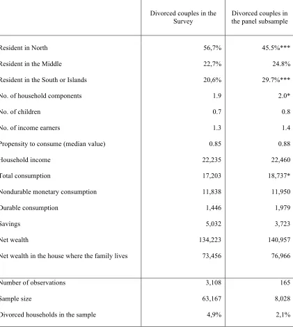
Table 8. A comparison between divorced couples in the whole SHIW dataset and the panel subsample employed for the analysis of this paper, year 1989-2006.

(average values)

Divorced couples in the Survey

Divorced couples in the panel subsample

Resident in North 56,7% 45.5%***

Resident in the Middle 22,7% 24.8%

Resident in the South or Islands 20,6% 29.7%***

No. of household components 1.9 2.0*

No. of children 0.7 0.8

No. of income earners 1.3 1.4

Propensity to consume (median value) 0.85 0.88

Household income 22,235 22,460

Total consumption 17,203 18,737*

Nondurable monetary consumption 11,838 11,950

Durable consumption 1,446 1,979

Savings 5,032 3,723

Net wealth 134,223 140,957

Net wealth in the house where the family lives 73,456 76,966

Number of observations

Sample size

Divorced households in the sample

3,108

63,167

4,9%

165

8,028

2,1%

Table 9. Regression analysis – Dependent variable: Logarithm of Nondurable Consumption

Independent variables Coefficients

Logarithm of household income 0.453***

0.019

Number of adults (aged more than 14) 0.033*** 0.009

Number of children 0.057***

0.009

The family owns even partially the house where it lives -0.183*** 0.016

The wife does not work out of home -0.052*** 0.018

The family lives in a southern region -0.059*** 0.017

The family will divorce within two years 1.146* 0.647

The family will divorce within two years * Logarithm of household income -0.111* 0.063

Time trend -0.028***

0.005

Squared time trend 0.002***

0.000

Constant 4.996***

0.195

Number of observations 2,317

R-squared 0.44