Window Effect in the Power Spectrum Analysis of a
Galaxy Redshift Survey
Takahiro Sato1, Gert Hütsi2, Gen Nakamura1, Kazuhiro Yamamoto1 1Graduate School of Physical Sciences, Hiroshima University, Higashi-Hiroshima, Japan
2Tartu Observatory, Tõrevere, Estonia Email: [email protected]
Received July 7, 2013; revised August 9, 2013; accepted August 16, 2013
Copyright © 2013 Takahiro Sato et al. This is an open access article distributed under the Creative Commons Attribution License, which permits unrestricted use, distribution, and reproduction in any medium, provided the original work is properly cited.
ABSTRACT
We investigate the effect of the window function on the multipole power spectrum in two different ways. First, we con- sider the convolved power spectrum including the window effect, which is obtained by following the familiar (FKP) method developed by Feldman, Kaiser and Peacock. We show how the convolved multipole power spectrum is related to the original power spectrum, using the multipole moments of the window function. Second, we investigate the de- convolved power spectrum, which is obtained by using the Fourier deconvolution theorem. In the second approach, we measure the multipole power spectrum deconvolved from the window effect. We demonstrate how to deal with the window effect in these two approaches, applying them to the Sloan Digital Sky Survey (SDSS) luminous red galaxy (LRG) sample.
Keywords: Cosmology; Large-Scale Structure of Universe
1. Introduction
One of the most fundamental problems in cosmology is the origin of an accelerated expansion of the Universe [1,2]. A hypothetical energy component, dark energy, may explain the accelerated expansion [3]. Modification of the gravity theory is an alternative way to explain it. In either case, this problem seems to be deeply rooted in the nature of fundamental physics, which has attracted many researchers. Dark energy surveys which aim at measur- ing redshifts of huge number of galaxies are in progress or planned [4,5]. These surveys provide us with a chance to test the hypothetical dark energy, as well as the gravity theory on the scales of cosmology. A key for distin- guishing between the dark energy and modified gravity theory is a measurement of the evolution of cosmological perturbations.
Galaxy redshift surveys provide promising ways of measuring the dark energy properties. Here, a measure- ment of the baryon acoustic oscillations in the galaxy distribution plays a key role. Also, the spatial distribution of galaxies is distorted due to the peculiar motions, which is called the redshift-space distortion. The Kaiser effect is the redshift-space distortion in the linear regime of the density perturbations. It is caused by the bulk mo- tion of galaxies [6]. The measurement of the Kaiser ef-
fect is thought to be useful for testing the general relativ- ity and other modified gravity theories [7-9]. In these analyses, measuring the multiple power spectrum in the distribution of galaxies plays a key role (cf. [10,11]).
The multipole power spectrum is useful for measuring the redshift-space distortion [12-18]. The usefulness of the quadrupole power spectrum to constrain modified gravity models is demonstrated in Refs. [19,20], as well as the dark energy model [21]. An estimator of the quad- rupole power spectrum is developed in Ref. [16]. How- ever, the disadvantage of the method is not being com- patible with the use of the fast Fourier transform (FFT). In the present paper, we consider different estimators of the quadrupole power spectrum which allows the use of the FFT. In this method, a full sample of a wide survey area is divided into smaller subsamples with equal areas. This approach was taken in Refs. [14,15]. In this case, the effect of the window function is crucial as we will show in the present paper. Thus, it must be properly ta- ken into account when comparing the observational data with theoretical predictions.
The convolved power spectrum includes the effect of
window effect into the multipole power spectra for the first time. We apply this formula to the Sloan Digital Sky Survey (SDSS) luminous red galaxy (LRG) sample from the data release (DR) 7, and investigate the behavior of the window function and its effect on the monopole and quadrupole spectra. We demonstrate how the window effect modifies the monopole spectrum and the quadru- pole spectrum. In the second half, we consider the de- convolved power spectrum, which is developed in Ref. [26], and compare it with the results of the first approach.
This paper is organized as follows: In Section 2, we briefly review the power spectrum analysis and the win- dow effect, where the convolved power spectrum is in- troduced. In Section 3, using the multipole moments of the window function, we derive the main formula to de- scribe how the convolved multipole power spectrum is related to the original power spectrum. Then, a method to measure the multipole moments of the window function is presented. We also apply the method to the SDSS LRG DR 7. In Section 4, the method for measuring the de- convolved power spectrum is reviewed. Then, a com- parison of the two approaches is given. Section 5 is de- voted to summary and conclusions. In the appendix, we give a brief review of a theoretical model, which we adopted. Throughout this paper, we use units in which the velocity of light equals 1, and adopt the Hubble pa- rameter H0100 km/s/Mpch with h0.7.
2. Basic Formulas of the FKP Method
Let us first summarize the power spectrum analysis de- veloped by Feldman, Kaiser and Peacock ([27], hereafter FKP). With this formulation we obtain the convolved power spectrum, including the window effect. We denote the number density field of galaxies by ng
s , where
ˆs z
s s is the three-dimensional coordinate in the (fiducial) redshift space, ˆs is the unit directional vector, and s z
is the comoving distance of a fiducial cos- mological model. According to Ref. [27], we introduce the fluctuation field
g
s
,F s n s n s (1) where ng
s
i
s s i
, with si being the locationof the ith object; similarly, ns
s is the density of asynthetic catalog that has a mean number density 1
times that of the galaxy catalog. In the present paper, we adopt 0.01. The synthetic catalog is a set of random points without any correlation, which can be constructed through a random process by mimicking the selection function of the galaxy catalog. For ng
s and ns
s ,we assume
1 2 1 2 1 2
1 1 2
1 ,
,
g g
n n n n
n
s s s s s s
s s s (2)
2
s 1 s 2 1 2
1
1 1 2 ,
n n n n
n
s s s s
s s s (3)
1
g 1 s 2 1 2 ,
n s n s n s n s (4)
where n
s denotes the mean number density of the galaxies, and
s s1, 2
is the two-point correlation func-tion. These relations lead to
1 2 1 2 1 2
1 1 2
,
1 .
F s F s n s n s s s
n s s s
(5)
We introduce the Fourier coefficient of F
s by
3 i
0 3 2 2 1 2
d , e
,
d ,
s F s
sn s
k s s k ks k (6)
where
s k, is the weight function (Throughout this paper, we assume 1). The expectation value of
2 0 k is
2 3 0 3 0 1 d 2π 1k P W
S
k k k k
k (7) with
2 i 33 2 2
, e d , d sn W sn
s k k
s s k
k k
s s k (8)
and
3 2
0 3 2 2
d , , d , sn S sn
s s k
k
s s k (9)
where we used
1 2 i 31 2 3
1
, d e .
2π kP
k s ss s k (10)
Here, W
k is the window function and S0
k isthe shotnoise. The estimator of the convolved power spectrum is taken
2
conv0 1 0 ,
P k F k S k (11) whose expectation value is
conv 3 3 1 d . 2πP k
k P k W k k (12) Hereafter, we omit , for simplicity.3. Convolved Power Spectrum
multipole power spectrum and the original multipole spectrum. We exemplify the behavior of the multipole moments of the window function and the convolved spectra, using the SDSS LRG sample from the DR 7. 3.1. Formulation
The estimator of the monopole power spectrum should be taken as
conv 3 conv
0 2 3 0 0 1 d 1
d (1 ) ,
k
Vk k
V k
P k kP
V k S V
k k k (13)where Vk is the volume of the shell in the k-space.
Similarly, a higher multipole power spectrum can be ob- tained [16]. Using the quantity
3 i
1 2
3 2 2
ˆ ˆ
d , e
, d s F sn
, k ss k s s k k
s s k (14)
where
is the Legendre polynomial, and kˆ is the unit wavenumber vector kˆk k , the estimator for the higher multipole power spectrum should be taken as (cf. [16])
conv 3 * 01 d 1 ,
k k V P k k S V
k k k
(15)
with
3 2
3 2 2
ˆ ˆ d , . d , sn S sn
s s k s k k
s s k (16)
The expectation value of Equation (15) is
conv
3 3
3
1 d 1 d ,
2π
k
k V
P k
k k P
V
k k k (17)
where we defined
1 2 13 2 2
i 3
1 1 1
i 3
2 2 2
2
d ,
d , e
d , e
. sn s n s n
s k k
s k k
k k s s k
s s k
s s k
s k
(18)
By adopting the distant observer approximation, we have
W
eˆˆ ,
k k k k k (19) and
conv 3 3 31 d 1 d ˆ ˆ ,
2π
k
k V
P k
k k P W
V
e
k k k k (20)
where ˆe is the unit vector along the line of sight. We consider the shell in the Fourier space whose outer (inner) radius is kmax
kmin
. The volume of the shell is Vk 2
4πk k where k
kmaxkmin
2 and k kmaxkmin,then
max min conv 2 ˆ 2 3 31 d d 1
4π 2π
ˆ ˆ .
k
k
P k kk
k k
d P W
e kk k k k k
(21)
Let us consider the limit k 0, then we have
conv ˆ 3 3 1 1 d 4π 2πˆ ˆ d . P k P W
e kk k k k k
(22)
Note that our definition of the multipole spectrum
P k is different from the conventional one by the factor 21 [12,13].
Now we introduce the coordinate variables to describe
k and k. For ˆe and kˆ, we adopt
0
sin cos 0
ˆ , sin sin , 1 cos k
e k (23)
respectively. As we consider the power spectrum and the window function averaged over the longitudinal variable around the axis of the direction eˆ, we may choose kˆ
so that 0 without loss of generality. Then, we choose the coordinate variable to describe k as
cos 0 sin sin cos 0 1 0 sin sin , sin 0 cos cos
k
k (24)
where and are the angle coordinates around kˆ
so as to be the polar axis. The matrix of the right hand side of Equation (24) denotes the rotation around the
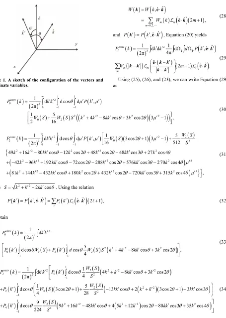
y-axis. See Figure 1 for the configuration. Note that
ˆ
ˆ sin sin cos cos cos ,
e k (25)
ˆ
ˆ cos ,
e k (26)
2 2 2 cos .
k k kk
Figure 1. A sketch of the configuration of the vectors and coordinate variables.
0,2, ˆ ˆ , ˆˆ 2 1 ,
m m
m
W W k
W k m
e e k k k (28)
and P
k P k
,eˆkˆ
, Equation (20) yields
conv 2 ˆ ˆ 31 d d 1 d ,ˆ ˆ
4π
2π
ˆ ˆ
ˆ
2 1 .
m m
m
P k k k d P k
W m
e e e k k k
k k
k k k
k k
(29)
Using (25), (26), and (23), we can write Equation (29) as
1 1 conv 2 0 20 1 1
2 2 2 2 2
0 2
1 d d cos d ,
2π
1 5
4 8 cos 3 cos 2 3 1 ,
2 16
P k k k P k
W S W S S k k kk k
(30)
1 1 2conv 2 2
2 2 0 2
0 1 1
2 2 2 2 2
2 2 2 2
1 d d cos d , 1 3cos 2 1 3 1 5
16 512
2π
49 16 80 cos 12 cos 2 48 cos 2 48 cos3 27 cos 4
42 96 192 cos 72 cos 2 288 cos 2 576 cos3 2 70 c
W S
P k k k P k W S
S
k k kk k k kk k
k k kk k kk k
22 2 2 2 2 4
os 4
81k 144k 432kk cos 180k cos 2 432k cos 2 720kk cos 3 315 cos 4k ,
(31)
where S k2k22kkcos. Using the relation
,ˆ ˆ
ˆ ˆ
2 1 ,
P P k
P k e
k s k k (32)
we obtain
conv 2 0 2 1 12 2 2 2
0 0 2 2
1 1
1 d 2π
5
d cos cos 4 8 cos 3 cos 2 ,
4
P k k k
P k W S P k d W S S k k kk k
(33)
1 2conv 2 2 2 2
2 2 0 2
1 1
2 2 2
2 0 2
1 1
2 2 2 2 2
4 2
1
1 1
d d cos 4 8 cos 3 cos 2
4 2π
1 5
d cos 3cos 2 1 13 cos 2 3cos 2 1 3 cos3
4 28
9
d cos 9 16 48 cos 4 5 12 c
224
W S
P k k k P k k k kk k
S W S
P k W S kk k k kk
S W S
P k k k kk k k
S
os 280kkcos335 cos 4k2
(34)
These formulas describe how the convolved spectra, c ( )
0 k
Ponv and c ( )
2 k
effect, compared with the original spectrum. Using Equa- tions (33) and (34), we define the quantity,
Pconv
k ,A k
P k
(35)
which is the correction factor connecting the original spectrum and the convolved power spectrum.
3.2. Measurement of the Multipole Moments of the Window Function
In this subsection, we explain a method to measure the multipole moment of the window function. The window function can be evaluated using the random catalog in a similar way of evaluating the power spectrum. Similar to the case of the power spectrum, we need to subtract the shotnoise contribution. Then, we adopt the following es- timator for the window function W
k , corresponding to the right hand side of Equation (8),
2
3 i
s
0
3 2 2
d ( , )e
d ( , )
s n
W S
sn
s k
s s k
k k
s s k (36)
We consider the window function expanded in the form of Equation (28). Mimicking the method to obtain the multipole power spectrum, we introduce
3s
1 2
3 2 2
ˆ ˆ
d , e
.
d ,
i
s n
sn
k s
s k s s k k
s s k (37)
and use the following estimator for the multipole mo- ment of the window function,
3
*
01 d .
k
k V
W k k N S
V
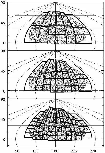
k k k (38) In the present work, we use the SDSS public data from the DR7 [28]. Our LRG sample is restricted to the red- shift range z=0.16 - 0.47 . In order to reduce the sidelobes of the survey window we remove some non- contiguous parts of the sample, which leads us to 7150 deg2 sky coverage with the total number N=100157 LRGs. The data reduction is the same as that described in Refs. [19,20,29,30]. In this subsection, we show general features of the window function of the LRG sample. In our approach, division of the full sample into subsamples is necessary because the line of sight direction is ap- proximated by one direction ˆe, and the distant observer approximation is required. Each subsample is distributed in a narrow area. We consider the three cases of the divi- sion, which are demonstrated in Figure 2. The full sam- ple is divided into 18, 32, and 72 subsamples, respec- tively. In those divisions of the full sample, each sub- sample has almost the same survey area, 398, 223, and 99 square degrees, respectively. Figure 2 shows the
cases divided into 18 subsamples, 32 subsamples and 72 subsamples. Figure 3 shows W k0
and W k2
as afunction of k, which are obtained by averaging the re- sults over all subsamples. As demonstrated in Figure 3,
0W k and W k2
can be fitted in the form,
0 4,
1
a W k
k b
(39)
2 2 4,
1
c W k
d k k e
(40) where the best fitting parameters a, b, c, d and e, which depend on the division of the full sample, are given in Table 1.
3.3. Measurement of the Convolved Power Spectrum
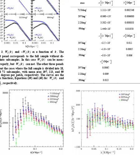
[image:5.595.317.532.332.644.2]Let us demonstrate the convolved multiple power spec- trum using the SDSS LRG sample from DR7. Figure 4
Figure 3. W k0
and W k2
as a function of k. The top left panel corresponds to the full sample without di- vision into subsamples. In this case W k0
can be meas- ured properly, but W k2
can not. The other three panels represent the cases where the full sample is divided into 18, 32, and 72 subsamples, with mean area 397, 223, and 99 square degrees per patch, respectively. The curves are the analytic functions, Equations (39) and (40) for W k0
and
2
W k , respectively.
Table 1. Values of the best fitting parameters for W k0
and W k2
in Equations (39) and (40), respectively.area a h
1Mpc
3 b h Mpc1
2
7150deg 1.111 10 9 0.002546
2
397deg 6.060 10 7 0.006680
2
223deg 3.382 10 7 0.008033
2
99deg 1.440 10 7 0.01050
1
3 Mpcc h
d h Mpc1
2
397deg 2.5 10 7 0.011
2
223deg 1.0 10 7 0.0085
2
99deg 3.0 10 6 0.006
1
Mpc
e h
2
397deg 0.0065
2
223deg 0.009
2
99deg 0.013
Figure 4. Convolved monopole power spectrum multiplied by the wavenumber conv
0kP k (left panel) and the quadrupole spectrum conv
2
kP k (right panel), respectively. In the left panel the curves from top to bottom correspond to the cases with no division of the full sample, to the division into 18, into 32, and into 72 subsamples, respectively. In the right panel, the results are for the cases with the division of the full sample into 18, into 32, and into 72 subsamples, respectively. The results with smaller subsamples have the smaller amplitude.
shows the monopole spectrum conv
0kP k (left panel) and the quadrupole spectrum conv
2
kP k (right panel), respectively. The results with different divisions of the
[image:6.595.83.533.127.626.2]the convolved power spectrum in Figure 4 is smaller for divisions with smaller patch sizes. Thus, the window effect is more influential for divisions with smaller patch- es.
Figure 5 plots A k0
defined by Equation (35) forthe monopole spectrum 0. The curves are obtained by computing Equation (33) with P k
corresponding to a spatially flat cold dark matter model with cosmo- logical constant and m 0.28, and with the window function shown in Figure 3. For the power spectrum we used the nonlinear model, Equation (50), given in the appendix, where the transfer function without the baryon oscillations is used [31], for simplicity. The three curves in Figure 5 assume different divisions of the full sample, whose patch sizes are shown in the legend.As shown in Figure 4, the amplitude of the convolved power spectrum depends on the division and the mean size of the subsamples. The amplitude becomes smaller when the mean patch area is reduced. Figure 6 shows the power spectrum conv
0 0
kP k A k , where A k0
is ob-tained by evaluating Equation (33), assuming the theo- retical model from Figure 5. The amplitude of the power spectra becomes almost the same, which means that the amplitude is correctly restored, i.e., the window effect is properly treated by Equation (33).
Figure 7 shows conv
2kP k for different divisions of the full sample, with mean patch sizes 397deg2 (a, left
panel), 223deg2 (b, center panel), 99deg2 (c, right
panel), respectively. The squares with error bars present
conv 2
kP k from the SDSS LRG sample, while the
Figure 5. conv
0 0 0
P k P k A k as a function of k for different divisions of the full sample. From the top to the bottom, the curves correspond to the cases with no division of the full sample, to the division into 18, 32, and 72 subsamples, respectively. Here, we assumed the ΛCDM cosmology with Ωm0.28, ns0.96, 80.8. The non- linear power spectrum model, Equation (50), with
370 km / s
v
is adopted.
Figure 6. Convolved monopole spectrum divided by the factor A k0
, i.e.,
conv
0 0
kP k A k .
Figure 7. Quadrupole power spectra multiplied by the wavenumber k for different divisions of the full sample, with mean survey areas 397deg2 (a, left panel), 223deg2 (b, center panel), and 99deg2 (c, right panel), respectively. The dotted curve is our theoretical model for kP k2
, while the dashed curve is conv
2
kP k from Equation (34), where we used the same theoretical model as that in Figure 3. The squares with the error bars present the observed convolved spectrum, conv
2
kP k . The dashes with the error bars show
conv
2 2
kP k A k .
dashes with error bars show conv
2 2
kP k A k , where
2A k is obtained by computing Equation (34) in the same way as A k0
. The dotted curves give the theo- retical model for kP k2
, where we used the same theo-retical model as that in Figure 5. The dashed curves are the corresponding conv
2
kP k , which are obtained by computing Equation (34). The ratio of the dashed curve to the dotted curve gives A k2
.4. Deconvolved Power Spectrum
4.1. Formulation
3 i conv
3 i 3 i
3 d e
1
d e d e .
2π
k P
k P k W
k sk s k s
k
k k (41)
The inverse transformation of
3 3 i conv
3 i3 i
d e
d e 2π
d e k P k P k W
k s k s k s k kk (42)
leads to
3 i 3 i conv
3 i
d e
d e .
d e k P P s k W
k s k s k s k kk (43)
In the case of a discrete density field of a galaxy cata- log, we must also take the shotnoise into account. The estimators for the convolved power spectrum and the window function are Equations (11) and (36), respec- tively. We choose the estimator for the deconvolved po- wer spectrum as
dec d e3 i U ,P s
Y
k s sk
s (44)
where we defined
2
3 i 3 i
3 2
d e d e
1 d
U k s F
s n
k s k s
s s s s (45)
23 i 3 i
3 2
d e e
d .
s
Y k d s n
s n
k s k s
s s s
s s
(46)
One can measure the deconvolved multipole power spectra from Equation (44) by
dec 1 d3 dec ˆ ˆ ,
k
l k V
P k kP
V
e k k (47) where Vk is a shell in the Fourier space. This decon-
volved multipole power spectrum can be compared with theoretical predictions directly without taking the win- dow effect into account.
4.2. Comparison between the Convolved Spectrum and the Deconvolved Spectrum
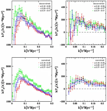
Figure 8 compares the convolved and deconvolved po- wer spectra of the LRG galaxy sample in the range of redshifts 0.16 < < 0.29z (red crosses), 0.29 < < 0.37z (blue bars) and 0.37 < < 0.47z (green squares). The left panels are the monopole spectra, while the right ones are the quadrupole spectra, multiplied by the wavenumber. The upper panels are the deconvolved power spectra, while the lower ones the convolved spectra, where we used the division of the full sample into 18 subsamples
with mean area 397 square degrees. The amplitude of the deconvolved spectrum is larger than that of the con- volved spectrum. Figure 9 shows the multipole moments of the window function of the LRG galaxy sample
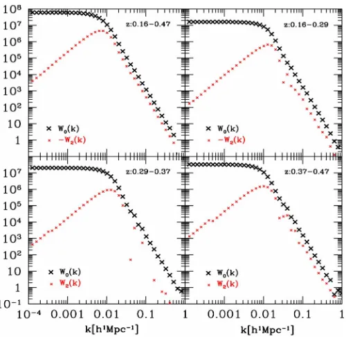
0W k (black large crosses) and W k2
(red small crosses) for the redshift ranges 0.16 < < 0.47z (upper left panel), 0.16 < < 0.29z (upper right panel),0.29 < < 0.37z (lower left panel), and 0.37 < < 0.47z (lower right panel), respectively. Here each redshift bin is divided into 18 angular subsamples whose mean area is 397 square degrees. The amplitude of W k0
in thelimit of small k is larger when the survey volume is larger. The sign of W k2
depends on the shape of thesubsamples.
4.3. Covariance Matrix
In the following we determine the covariance matrices by utilizing mock catalogs corresponding to the SDSS LRG sample. Our mock catalogs are built by following the procedure described in Ref. [29]. The covariance matrices for the multipole spectra are defined by
,
.
i j i j
i i j j
C k k P k P k
P k P k P k P k
(48)
The correlation matrices, which describe the correla- tions between different wavenumbers, are defined by
i, j
i, j
i, i
j, j
. [image:8.595.60.287.79.244.2]r k k C k k C k k C k k (49)
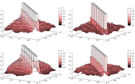
Figure 10 shows the correlation matrices of the mono- pole spectrum, r k k0
i, j
, on the ki and kj plane (kis in units of hMpc1), which are computed from 1000
mock catalogs. The left panels are for the convolved spectra, while the right ones for the deconvolved power spectra. The top panels show the case without the divi- sion of the full sample, while the other panels (from bot- tom to top) represent the cases when the full sample is divided into subsamples, whose mean patch sizes are 99, 223 and 397 degrees, respectively. One can see that the off-diagonal components of the correlation matrices for the convolved spectrum are larger if the mean area of the subsample gets smaller. One can also find that the off- diagonal components for the deconvolved spectrum get reduced due to the deconvolution. The off-diagonal com- ponents of the correlation matrix for the deconvolved spectrum are not completely reduced to zero for the cases with the subsamples whose mean patch sizes are small.
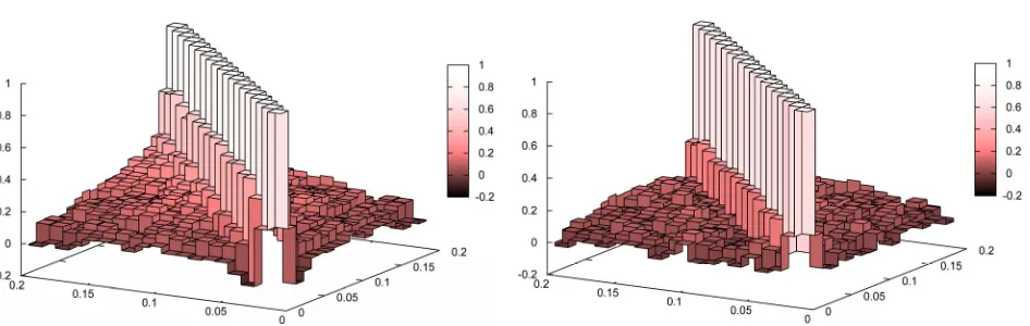
Figure 11 shows the correlation matrices for the quad- rupole spectrum r k k2
i, j
. Similar to Figure 10, the left [image:8.595.61.289.329.470.2]full sample is divided into the subsamples, whose mean areas are 99, 223 and 397, respectively, from the bottom to the top panels. Similar to the case of the correlation matrix of the monopole spectrum, we see that the corre- lation between the different wavenumbers becomes sig- nificant for the case when the full sample is divided into smaller subsamples. The effect is more significant when the mean area of the subsample gets smaller. The corre- lation between the different wavenumbers is practically de-correlated while using the deconvolved power spec- trum. Despite of the window deconvolution, the correla- tion between the different wavenumbers remains notice- able when the mean area of the subsample is small. These features are common to the correlation matrices of the monopole.
5. Summary and Conclusions
The window effect is very crucial when the power spec- trum analysis is done by dividing the full sample into small subsamples. The division is necessary for obtaining the higher order multipole spectra within the distant ob- server approximation using the FFT. It is possible to compute the higher multipole spectra without the divi- sion of the full sample [16]. In that case the window ef- fect is not so significant, however, the FFTs cannot be applied. The usage of the FFT is quite useful for per- forming the Fourier transform quickly. Thus, the tech- nique for the treatment of the survey window in the power spectrum analysis will be quite important.
We investigated the effect of the window function on the multipole power spectrum via two different approaches. In the first approach, we gave the theoretical formula for the convolved multipole power spectra, Equations (33) and (34), which can be computed by measuring the mul- tipole moments of the window function. The multipole moments of the window function were measured with the SDSS LRG sample, using the various divisions of the full sample into subsamples. The second approach is the measurement of the power spectrum deconvolved from the window effect. The advantage of the deconvolved power spectrum is the simplicity while comparing with theoretical models. The approximate de-correlation be- tween the modes with different wavenumbers is also the advantage of the deconvolved power spectrum. We de- monstrated the differences between these two approaches to dealing with the window effect for the multipole po- wer spectrum.
6. Acknowledgements
This work was supported by Japan Society for Promotion of Science (JSPS) Grants-in-Aid for Scientific Research (Nos. 21540270, 21244033). This work was also sup- ported by JSPS Core-to-Core Program “International
Research Network for Dark Energy”. This work was done when T. Sato and G. Nakamura were Ph.D. students of Graduate School of Physical Sciences, Hiroshima University.
REFERENCES
[1] S. Perlmutter, et al., “Measurements of Ω and Λ from 42 High-Redshift Supernovae,” The Astrophysical Journal, Vol. 517, No. 2, 1999, p. 565 [2] A. G. Riess, et al., “Observational Evidence from Super-
novae for an Accelerating Universe and a Cosmological Constant,” The Astrophysical Journal, Vol. 116, No. 3, 1998, p. 1009
[3] P. J. E. Peebles and B. Ratra, “The Cosmological Con- stant and Dark Energy,” Reviews of Modern Physics, Vol. 75, No. 2, 2003, pp. 559-606.
[4] A. Albrecht, et al., “Report of the Dark Energy Task Force,” 2006. arXiv:astro-ph/0609591
[5] J. A. Peacock, et al., “ESA-ESO Working Group on Fun- damental Cosmology,” 2006. arXiv astro-ph/0610906 [6] N. Kaiser, “Clustering in Real Space and in Redshift
Space,” Monthly Notices of the Royal Astronomical Soci-ety, Vol. 227, 1987, pp. 1-21.
[7] E. V. Linder, “Redshift Distortions as a Probe of Grav- ity,” Astroparticle Physics, Vol. 29, No. 5, 2008, pp. 336- [8] L. Guzzo, et al., “A Test of the Nature of Cosmic Accel- eration Using Galaxy Redshift Distortions,” Nature, Vol. 451, 2008, pp. 541-544. [9] R. Reyes, et al., “Confirmation of General Relativity on
Large Scales from Weak Lensing and Galaxy Velocities,” Nature, Vol. 464, 2010. pp. 256-258.
[10] T. Okumura, et al., “Large-Scale Anisotropic Correlation Function of SDSS Luminous Red Galaxies,” The Astro- physical Journal, Vol. 676, No. 2, 2008, p. 889.
[11] A. Cabre and E. Gaztanaga, “Clustering of Luminous Red Galaxies—I. Large-Scale Redshift-Space Distortions,” Month- ly Notices of the Royal Astronomical Society, Vol. 393, No. 4, 2009, pp. 1183-1208.
[12] S. Cole, K. Fisher and D. H. Weinberg, “Fourier Analysis of Redshift Space Distortions and the Determination of Omega,” Monthly Notices of the Royal Astronomical So-ciety, Vol. 267, 1994, pp. 785-799.
[13] A. J. S. Hamilton, “The Evolving Universe,” Kluwer Aca- demic Publishers, Dordrecht, 1998.
[14] P. J. Outram, et al., “The 2dF QSO Redshift Survey—VI. Measuring Λ and β from Redshift-Space Distortions in the Power Spectrum,” Monthly Notices of the Royal Astro- nomical Society, Vol. 328, No. 1, 2001, pp. 174-184.
A Measurement of Λ from the Quasi-Stellar Object Power Spectrum, PS(k
//, k⊥),” Monthly Notices of the Royal Astro- nomical Society, Vol. 348, No. 3, 2004, pp. 745-752.
[16] K. Yamamoto, M. Nakamichi, A. Kamino, B. A. Bassett and H. Nishioka, “A Measurement of the Quadrupole Power Spectrum in the Clustering of the 2dF QSO Sur- vey,” Publications of the Astronomical Society of Japan, Vol. 58, 2006, pp. 93-102. 415, No. 3, 2011, pp. 2876- 2891.http://pasj.asj.or.jp/v58/n1/580114/58012766.pdf [17] C. Blake, et al., “The WiggleZ Dark Energy Survey: The
Growth Rate of Cosmic Structure Since Redshift z = 0.9,” Monthly Notices of the Royal Astronomical Society, Vol. 415, No. 3, 2011, pp. 2876-2891.
[18] A. Taruya, S. Saito and T. Nishimichi, “Forecasting the Cosmological Constraints with Anisotropic Baryon Acous- tic Oscillations from Multipole Expansion,” Physical Re- view D, Vol. 83, No. 10, 2011, Article ID: 103527.
[19] K. Yamamoto, T. Sato and G. Hütsi, “Testing General Relativity with the Multipole Spectra of the SDSS Lumi- nous Red Galaxies,” Progress of Theoretical Physics, Vol. 120, No. 3, 2008, pp. 609-614 [20] K. Yamamoto, G. Nakamura, G. Huetsi, T. Narikawa and
T. Sato, “Constraint on the Cosmological f(R) Model from the Multipole Power Spectrum of the SDSS Lumi- nous Red Galaxy Sample and Prospects for a Future Redshift Survey,” Physical Review D, Vol. 81, No. 10, 2010, Article ID: 103517.
[21] K. Yamamoto, B. A. Bassett and H. Nishioka, “Dark Ener- gy Reflections in the Redshift-Space Quadrupole,” Phy- sical Review Letters, Vol. 94, No. 5, 2005, Article ID: 051301.
[22] W. Percival, et al., “Baryon Acoustic Oscillations in the Sloan Digital Sky Survey Data Release 7 Galaxy Sam- ple,” Monthly Notices of the Royal Astronomical Society, Vol. 401, No. 4, 2010, pp. 2148-2168.
[23] B. A. Reid, et al., “Thick Gas Discs in Faint Dwarf Gal-
axies,” Monthly Notices of the Royal Astronomical Soci- ety, Vol. 404, No. 1, 2010, pp. L60-L63.
[24] W. Percival, et al., “The Shape of the Sloan Digital Sky Survey Data Release 5 Galaxy Power Spectrum,” The As- trophysical Journal, Vol. 657, No. 2, 2007, p. 645. [25] S. Cole, et al., “The 2dF Galaxy Redshift Survey: Power-
Spectrum Analysis of the Final Data Set and Cosmologi- cal Implications,” Monthly Notices of the Royal Astro- nomical Society, Vol. 362, No. 2, 2005, pp. 505-534.
[26] T. Sato, G. Hütsi and K. Yamamoto, “Deconvolution of Window Effect in Galaxy Power Spectrum Analysis,” Pro- gress of Theoretical Physics, Vol. 125, No. 1, 2011, pp. 187-197.
[27] H. A. Feldman, N. Kaiser and J. A. Peacock, “Power- Spectrum Analysis of Three-Dimensional Redshift Sur- veys,” Astrophysical Journal, Vol. 426, No. 1, 1994, pp. [28] K. N. Abazajian, et al., “The Seventh Data Release of the Sloan Digital Sky Survey,” The Astrophysical Journal Sup- plement Series, Vol. 182, No. 2, 2009, p. 543.
[29] G. Hütsi, “Acoustic Oscillations in the SDSS DR4 Lu- minous Red Galaxy Sample Power Spectrum,” Astron- omy & Astrophysics, Vol. 449, No. 3, 2006, pp. 891-902.
[30] G. Hütsi, “Power Spectrum of the SDSS Luminous Red Galaxies: Constraints on Cosmological Parameters,” As- tronomy & Astrophysics, Vol. 459, No. 2, 2006, pp. 375-
[31] J. M. Bardeen, J. R. Bond, N. Kaiser and A. S. Szalay, “The Statistics of Peaks of Gaussian Random Fields,” The Astrophysical Journal, Vol. 304, 1986, pp. 15-61. [32] J. A. Peacock and S. J. Dodds, “Reconstructing the Linear
Power Spectrum of Cosmological Mass Fluctuations” Monthly Notices of the Royal Astronomical Society, Vol. 267, 1994, pp. 1020-1034.
Theoretical Model for the Power Spectrum
In this appendix, we explain the theoretical models adopt- ed in the present paper. The simplest model for the gal- axy power spectrum in the redshift-space is
2
2
gal , nl v ,
P k b k f P k D k (50)
where b k
is the clustering bias, P knl
is the non-linear matter power spectrum, D
vk
is the damp-ing factor due to the finger of god effect, and v is the
pair wise velocity dispersion. Assuming an exponential distribution function for the pairwise velocity, the damp- ing function is
2 21 2 .1 2
v
v
D k
k
For the nonlinear matter power spectrum P knl
, we [image:11.595.87.514.210.656.2]adopt the fitting formula by Peacock and Dodds (1994) [32].
Figure 9. The window functions W k0
(black crosses) and W k2
(red small crosses) assuming the full sample is divided into subsamples with redshift ranges, 0.16 < < 0.29z (upper right panel), 0.29 < < 0.37z (lower left panel) and0.37 < < 0.47z (lower right panel), which correspond to the analysis of Figure 1. The upper left panel is the case using the full redshift range 0.16 < < 0.47z , which is the same as the upper right panel of Figure 3.
[image:13.595.64.538.77.373.2]
Figure 10. Correlation matrices of the monopole spectrum, r k k0
i, j
, for the convolved spectrum (left panels) and thedeconvolved spectrum (right panels), respectively, on the ki and kj plane (k in units of 1 Mpc
h ). The top panels show the case with no division of the full sample, while the other lower panels (from bottom to top) show the cases when the full sample is divided into subsamples, whose mean area is 99, 223 and 397 square degrees, respectively.
Figure 11. Correlation matrices of the quadrupole spectrum, r k k2