Munich Personal RePEc Archive
Financial Development and Income
Inequality: Is there any Financial
Kuznets curve in Iran?
Muhammad, Shahbaz and Tiwari, Aviral and Reza,
Sherafatian-Jahromi
COMSATS Institude of Information Technology, Lahore, Pakistan,
Tripura University, University Putra Malaysia
20 August 2012
Online at
https://mpra.ub.uni-muenchen.de/40899/
Financial Development and Income Inequality: Is there any Financial Kuznets curve in Iran?
Muhammad Shahbaz
Department of Management Sciences, COMSATS Institute of Information Technology, Lahore, Pakistan. Email: shahbazmohd@live.com www.ciitlahore.edu.pk, UAN: 0092-42-111-001-007,
Fax: 0092-42-99203100, Mobile: +92334-3664-657
Aviral Kumar Tiwari
Faculty of Applied Economics,
Faculty of Management, ICFAIUniversity, Tripura, Kamalghat, Sadar, West Tripura, Pin-799210, Email: aviral.eco@gmail.com&aviral.kr.tiwari@gmail.com
Reza Sherafatian-Jahromi
Department of Economics, University Putra Malaysia, 43400UPM Serdang, Selangor, Malaysia
Email: rezasherafatian@yahoo.com
Abstract
This deals with the investigation of the relationship between financial development and income inequality in case of Iran. In doing so, we have applied the ARDL bounds testing approach to examine the long-run relationship in the presence of structural break stemming in the series. The unit root properties have been tested by applying Zivot-Andrews (1992) and Clemente et al. (1998) structural break tests. The VECM Granger causality approach is used to detect the direction of causal relationship between financial development and income distribution. Moreover, Greenwood-Jovanovich (GJ) hypothesis has also been tested for Iranian economy.
Our results confirm the long run relationship between the variables. Furthermore, financial development reduces income inequality. Economic growth worsens income inequality, but inflation and globalization improve income distribution. Finally, GJ hypothesis is found as well as U-shaped relationship between globalization and income inequality in case of Iran. This study might provide new insights for policy makers to reduce income inequality by making economic growth more fruitful for poor segment of population and directing financial sector to provide access to financial resources of poor individuals at cheaper cost.
Introduction
Higher economic growth with equal income distribution is a great matter of concern for all
developing economics; those are trying to catch-up the growth path of developed countries,
which is true for Iranian economy too. It has been verified by numerous empirical studies, for
different countries, that for a developing country (in particular), which is trying to attain a
high economic growth rate, that inequality on various grounds increases with the growth of
an economy (Chambers et al. (2007 and, Baliscan and Fuwa, 2005). Our observation on the
Gini coefficient and GDP per-capita (see figure 1 and figure 3 respectively) provides a clue
for such a situation to exist in Iran too. We find from Figure-1 that the Gini coefficient was
increased initially and thereafter it has shown fluctuating trends. The correlation between
economic growth and income inequality is positive i.e. 0.2691 and negative i.e. 0998 between
financial development and income inequality. By looking into trend of GDP per-capita we
observe that it has initially increased, then decreased and now again has moved up word.
Recognizing the problems associated with the increasing inequality, Iranian’s government
has taken various steps to combat with income inequality in order to mitigate negative
consequences that might arise due to it. To combat with the inequality a prudential
development of financial sector can be used as a big tool. Development and proper
management of the financial sectors help in the faster and sustained economic growth. First,
for example, easy access to financial resources boosts investment activities that directly
increase the income of poor segments of population by generating employment opportunities.
Second, easy access to financial resources provides various opportunities and enables the
poor segments of population among other to increase human capital formation by investing in
education, health and various aspects of socio-economic development of their children and
family members. Third, financial development reduces income and wealth inequalities and
mitigates various problems, which arises due to increasing inequality of such type and so on
might also be helpful in protecting the indexed income of the elite class via easy access to
financial resources during the instances of high inflations since inflation is very harmful for
those who earn fixed income as high inflation reduces their purchasing power.
However, as Greenwood and Jovanovich, (1990) argued that initially financial development
increases income inequality but declines income inequality once financial sector matures.
This seems to be holding of inverted U-shaped hypothesis between financial development
and income inequality. There is another mechanism through which financial sector may
improve income distribution which is known as down effect”. According to
“trickle-down effect”, as economies expand, poverty is likely to be reduced but poverty reduction is
likely to be adversely affected due to increased income inequality.
Income inequality is one of those problems that most of less developed countries have been
facing for a long time. Slottje and Raj, (1998) showed that in South America and Asia, there
is the worst income distribution while in Europe, income inequality is low. By a simple
comparison between Iran and North Americas, Europe and Oceans in their study, it can be
concluded that income inequality is high in Iran as compared to these regions. Over the years,
it is observed that income inequality (Gini-coefficient) has fluctuated in Iran–(see Figure-1).
It can be seen that from 1971 to 1975 Gini coefficient in Iran was increased. One of the most
important reasons for this was increase in oil shock. After that and until 1978 it decreased
slightly due to increase in import and subsidies. From 1979 to 1988 Iran had faced with
revolution, war and economical restriction which affected income inequality. From 1985 to
1987 income inequality increased which could be the result of decreasing in oil income. After
this period, war is terminated and Gini-coefficient diminished till 1992 but in 1993 Iran faced
also been seen after 1997. Figure (2) belongs to real GDP per capita in Iran. This figure
shows that most of the time real GDP per capita has an upward trend in Iran. But we didn’t
see a downward trend in Gini-coefficient and better income distribution was in this period.
Figure-1: Gini Coefficient in Iran
Figure-2: Real GDP Per Capita in Iran
1000000 2000000 3000000 4000000 5000000 6000000 7000000 8000000
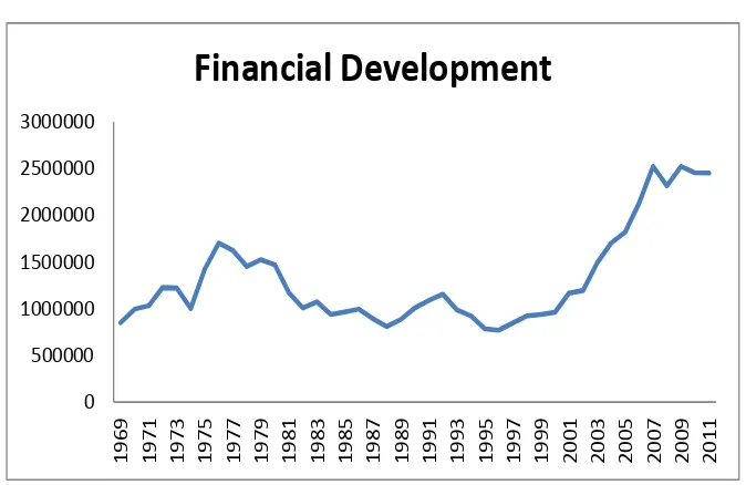
Figure-3: Financial Development in Iran
0 500000 1000000 1500000 2000000 2500000 3000000
19
69
19
71
19
73
19
75
19
77
19
79
19
81
19
83
19
85
19
87
19
89
19
91
19
93
19
95
19
97
19
99
20
01
20
03
20
05
20
07
20
09
20
11
Financial
Development
As it can be seen from figure (2), real GDP per capita rose before Iran’s revolution, but after
revolution it decreased. Revolution and war on the one hand and increasing in population on
the other hand were the main factors for this decline. Increasing in production and
diminishing in growth rate of population helped Iran’s economy to increase its real GDP per
capita in last decade of twentieth century and first decade of third millennium.
Figure (3) shows domestic credit to private sector per capita which is a proxy for financial
development in Iran. Financial sector development began deteriorating after 1977 for a
decade, remained relatively low in 1994 to1996 but gradually improved in subsequent years.
Upward trend can be seen for this variable before the 1977, but after this time it started to
decrease. This declining could be because of nationalizing and merging of banks. Moreover,
increasing in invisible trade could be another reason. After war, Iran tried to develop his
financial sector by launching 5 years development plan.From 1996 we can see an upward
started their job. Iran in its last 5 years development plan allowed the non-Iranian banks to
open their branches to improve the efficiency of financial sector.
In the recent years there is increasing interest of researchers to analyze economic
consequences of financial development on income inequality at national and cross-country
levels. However, Iran has been departed from such research. The present study is intended to
fill this gap. This paper contributes to existing literature by four folds: (i) the nexus between
financial development and income inequality is investigated by using time series data in case
of Iran, (ii), unit root properties of the variables have been examined by applying structural
break unit root tests such as Zivot-Andrews (1992) and Clemente et al. (1998), (iii), in doing
so, we have applied the structural break ARDL bounds testing approach to cointegration for
long run relationship between the variables and, (iv) the VECM Granger causality is applied
to test causal relation between the variables.
This paper is structured as follows. Section-II, presents a brief review of literature on
relationship between financial development and income inequality. Modeling,
methodological framework and data collection are presented in Section-III. Section-IV deals
with results interpretation, and Section-V draws conclusion and policy recommendations.
II: Literature Review
Over the last three decades, there is growing interest of researchers on analyzing the financial
development and economic growth (Pagano, (1993); Levine, (1997); Levine et al. (2000);
Anderson and Tarp, (2003); Jalilian and Kirkpatrick, (2005)). Levine, (1997) confirms that
long run economic growth has been experienced by those economies which have well
Kirkpatrick, (2000) showed the role of well-functioning financial system in mobilization of
savings, resource allocation, and facilitation of risk management which in turn provides
support for capital accumulation, improves efficiency of investment and promotes
innovations in technology and hence contributes to economic growth. Similarly; Goldsmith,
(1969); Mckinnon, (1973); King and Levine, (1993); Pagano and Volpin, (2001);
Christodoulou and Tsionas, (2004); Shan, (2005); Ma and Jalil, (2008) and Shahbaz et al.
(2010) paid their attention to identify the degrees as well as effectiveness of financial
development on sustained economic growth, physical capital accumulation and economic
efficiency.
Our concern is to discuss the relationship between financial development and income
inequality. There are various studies which have highlighted various aspect of association of
financial development and income inequality. For example, Galor and Zeira (1993), and
Banerjee and Newman (1993) have highlighted that financial markets particularly credit
market improve income distribution. They suggested that the initial income gap would not be
reduced unless financial markets are sound. Similarly, Canavire-Bacarreza and Rioja, (2009)
document that “given their lack of collateral and scant credit histories, poor entrepreneurs
may be the most affected by financial market imperfections such as information asymmetries,
contract enforcement costs, and transactions costs”.
There are some other ways also through which financial development may increase income
inequality. For example, as Behrman et al. (2001); Dollar and Karaay, (2003); Beck et al.
(2004) mentioned that in the early stage of financial development, financial sector may
charge high set up cost against financial services during to gain advantages from the
individuals are unable to come out from the circle of income inequality. Further, deficiencies
in money markets in terms of asymmetric information, intermediation and transaction costs
restrict the poor people to attain loans from financial institutions because they do not have
collateral, credit records and political; and personal connections with high authorities of
financial sector to get loans at reasonable interest rate. Hence, even if there is enough funds to
be distributed at reasonable rate of interest among poor people then they are unable to avail
benefit of such services. Claessense, (2006) and Perotti, (1996) provided another reason due
to which poor people are unable to access the benefit of financial development. They argued
that since poor individuals are not much educated and formal financial sector does not seem
to prefer such un-educated or less-educated persons to offer loans and hence in many high
income countries, financial sector has dualism in financial services.
Galor and Zeira, (1993) argued that access of poor entrepreneurs to financial resources
enables them to start small to enhance their earnings. This not only reduces income inequality
and hence declines poverty. On contrarily, Bourguignon and Verdier, (2000) noticed that
since in almost cases, poor rely more on informal networks for credit hence, financial
development would only benefit the rich class of the society and raises income inequality.
Greenwood and Jovanovich, (1990) proposed a non-linear relationship between financial
development and income inequality or what we may call as “inverted-U” hypothesis. They
argued that initially financial development increases income inequality and improves income
distribution once financial sector matures.
Furthermore; Westley, (2001) investigated the impact of financial markets on income
distribution for Latin American countries in panel framework and reported that easy access to
Serven, (2003) disclosed that financial development worsens income distribution while
education improves it. Similarly, Lopez, (2004) also found that better education and low
prices seem to decrease income inequality. Financial development, international trade and
government size hamper income distribution. Similarly; Honohan, (2004); Beck et al. (2004);
Stijn and Perotti, (2007) noticed that financial development and income inequality is not only
a correlation but also a causal relationship between both variables. For example, positive
impact of financial development on economic growth may enable the poor segments of
population to demand for loans from financial markets to increase their income levels as
economy grows. However, Beck et al. (2007a) documented that strong relationship between
finance and growth does not necessarily mean that financial development improves income
distribution and hence reduces poverty. They claimed that financial development will help
decline poverty if financial development increases average income of both rich and poor
segments with of population. Financial development will help the poor if average income is
higher achieved by rich class. On the other hand, Li et al. (1998) found that financial
development lowers income inequality by raising the average income of bottom 20%
population. Beck et al. (2007b) using cross-country data, found that financial development
raises income of poor segment of population disproportionately and reduces income
inequality. On contrary; Bonfiglioli, (2005) used cross-country data to examine the impact of
financial development proxies by stock market development on income inequality and
concluded that financial development has progressive effect on income inequality.
In case country studies; Liang, (2006) reported that financial development improves urban
income distribution in post-reform China. In case of Malaysia; Law and Tan, (2009)
examined the role of financial development in affecting income inequality. They used stock
Their results supported favorable impact of financial development on income distribution
while inflation raises income inequality. Shahbaz, (2009) used Pakistani data to examine the
impact of financial development and financial instability on the income of bottom 20%
population. The results indicted that financial development increases the income poor
segment of population but this effect is nullified by financial instability. In case of India;
Ang, (2010) investigated relationship between both variables and concluded that financial
development helps reduce income inequality but financial liberalization deteriorates income
distribution. Using Brazilian data, Bittencourt, (2010) investigated the impact of financial
development on income inequality and found that financial development declines income
inequality by increasing income bottom 20% population. Shahbaz and Islam, (2011) probed
the relationship between financial development and income distribution in the presence of
financial instability in case of Pakistan. Their results indicated that financial development
declines income inequality while financial instability worsens income distribution.
Moreover; Wahid et al. (2011) found that financial development increases income inequality
in case of Bangladesh. Furthermore, results revealed that economic growth improves income
distribution suggesting that improvements in economic growth redistribute income and make
the society more egalitarian. Using Bayesian structural autoregressive model (SVAR), Gimet
and Lagoarde‐Segot, (2011) reexamined the relationship between financial development and
income inequality. They uncovered that financial development Granger causes income
distribution. In case of China, Jalil and Feridun, (2011) questioned whether financial
development improves income distribution or not. Their results accepted inequality
narrowing hypothesis implying that financial development reduces income inequality. In case
of Indian states, Arora, (2012) raised the issue of finance-inequality nexus for empirical
development. Financial development improves inequality in rural but raises inequality in
urban areas. Yu and Qin, (2011) also supported the fact that financial development helps to
reduce rural-urban income gap in China. Similarly, Chun and Peng, (2011) reported favorable
impact of financial development on income distribution. They suggested that government
should loosen financial regulations, and lower market anticipation level to ensure the whole
society can take advantage of economy development; open the financial market to higher
degree, and promote the competition; accelerate interest rate marketization; build up a
financial system which facilitates SMEs financing; develop micro-financial institutions and
micro loans; develop technology and its application in financial areas, in order to lower
financial cost; develop the financial industry support on human capital investment. Iyigun
and Owen, (2012) found that financial development affects income inequality by controlling
aggregate consumption variability. In low income countries, income inequality is linked with
more consumption volatility and vice versa in high income countries. Hamori and
Hashiguchi, (2012) documented that impact of financial development on income inequality
depends on the choice of financial variables.
Various studies are available investigating GJ (1990) hypothesis between financial
development and income inequality. For example; Li et al. (2008) investigated the
relationship between financial development and income inequality and confirmed the
existence of U-shaped Kuznets curve for East Asian countries while Rehman et al. (2008),
while working on in similar line; reject inverted U-shaped relationship between financial
development and income inequality. Sebastian and Sebastian, (2011) probed the relationship
between financial development and income inequality by applying fixed effects model1. Their
1
results indicated that financial development worsens income inequality but could not find
existence of GJ (1990) hypothesis between both the variables. Kim and Lin, (2011) noted that
financial development improves income distribution if country achieves the threshold level of
financial development and below this level financial development worsens income inequality
i.e. GJ (1990) hypothesis and same inference is drawn by Rötheli, (2011). Shahbaz and Islam,
(2011) also found U-shaped relationship between financial development and income
inequality in Pakistan but it is statistically insignificant.
Batuo et al. (2012) investigated the empirical existence of GJ (1990) hypothesis using data of
African countries applying dynamic panel estimation technique (GMM)2. They found that
financial development has positive impact on income distribution but could not find evidence
supporting the GJ (1990) hypothesis or inverted U-shaped relationship between financial
development and income inequality. Nikoloski, (2012) investigated the linear and non-linear
relationship between financial development and income inequality applying system
generalized moments method (GMM)3. His empirical evidence proved the existence of
inverted-shaped relationship between financial development and income equality i.e. GJ
(1990) hypothesis. Tan and Law, (2012) investigated the dynamics of finance-inequality
Guyana, Grenada, Hong Kong, Hungary, Honduras, Iceland, India, Indonesia, Iran, Ireland, Israel, Italy, Jamaica, Japan, Jordan, Kazakhstan, Korea, Rep. Latvia, Lithuania, Lesotho, Luxembourg, Malta, Macedonia, Malaysia, Mauritius, Mexico, Moldova, Mongolia, Morocco, Netherlands, New Zealand, Nigeria, Norway, Pakistan, Papua New Guinea, Paraguay, Philippines, Panama, Peru, Poland, Portugal, Romania, Russian Federation, Senegal, Sri Lanka, Swaziland, Serbia, Seychelles, Singapore, Slovak Republic, Slovenia, Spain, South Africa, St. Lucia, St. Vincent and the Gren, Suriname, Sweden, Switzerland, Turkey, Thailand, Tunisia, Trinidad a. Tobago, United Kingdom, United States, Uruguay, Venezuela RB, Vietnam, Yemen, Rep.
2
Botswana, Ivory Coast, Cameroon, Egypt, Ethiopia, Ghana, Kenya, Lesotho, Morocco, Madagascar, Mauritania, Mauritius, Malawi, Nigeria, Senegal, Sierra Leone, South Africa, Tanzania, Tunisia, Uganda, Zambia and Zimbabwe.
3
nexus using data of 35 countries4. Their results indicated U-shaped relationship between
financial deepening and income distribution. This implies that financial markets are
inefficient to improve income distribution in these countries. In case of China, Ling-zheng
and Xia-hai, (2012) applied threshold model developed by Hansen, (1999) using provincial
data to investigate the relationship between financial development and income inequality.
Their results disclosed that financial development deteriorates income inequality and
supported the existence of U-shaped relationship between both variables.
III- Modeling, Methodological Framework and Data Collection
The objective of this study is to examine the relationship between financial development and
income inequality including economic growth, inflation and globalization are other potential
determinates of income inequality in case of Iran. The general functional form of model is
given below as following:
)
,
,
,
(
t t t tt
f
Y
F
IN
G
IE
(1)In this equation, IEt is income inequality, Yt shows economic growth, Ft illustrates
financial development, INt represents inflation, andGtis globalization. We have converted
all the series into logarithm for consistent and reliable results. The log-linear specification
provides better results because conversion of the series into logarithm reduces the sharpness
in time series data (Shahbaz, 2010). The empirical equation is modeled as following:
i t t
t t
t Y F IN G
IE
ln
ln
ln
ln
ln 1 2 3 4 5 (2)
4
where, lnIEt, lnYt, lnFt, lnINt, lnGtis natural log of income inequality proxies by
Gini-coefficient, natural log of economic growth measured by real GDP per capita, natural log of
financial development captured by real domestic credit to private sector per capita, natural
log of inflation proxies by consumer price index, natural log of globalization measured by
KOF globalization index (following Dreher, 2006). is residual term containing normal
distribution with finite variance and zero mean. To test the GJ hypothesis following
non-linear specification is considered:
t t t
t t
t
t Y F F IN G
IE
ln
ln
ln
ln
ln
ln 55 66
2 44 33
22
11 (3)
Equation-3 envisages inequality reducing hypothesis if 33 0keeping44 0. Income
inequality increases if 33 0and 44 0. The GJ (1990) hypothesis would be confirmed if
0 33
and 44 0otherwise U-shaped relationship between financial development and
income inequality is accepted if 33 0and 44 0. Similarly, nonlinear relationship
between globalization and income inequality is investigated by including squared term of
t
G
ln i.e. lnGt2. The empirical equation is modelled as following:
t t t
t t
t
t Y F IN G G
IE 2
66 55
44 33
2
11 ln ln ln ln ln
ln (4)
The inverted-U shaped theory would be accepted if 55 0and 066 otherwise U-shaped
relationship between globalization and income inequality is accepted if 55 0and 66 0.
Numerous unit root tests are available on applied economics to test the stationarity properties
of the variables. These unit tests are ADF by Dickey and Fuller (1979), P-P by Philips and
Ng-Perron by Ng-Ng-Perron (2001). These tests provide biased and spurious results due to not
having information about structural break points occurred in series. In doing so,
Zivot-Andrews (1992) developed three models to test the stationarity properties of the variables in
the presence of structural break point in the series: (i) this model allows a one-time change in
variables at level form, (ii) this model permits a one-time change in the slope of the trend
component i.e. function and (iii) model has one-time change both in intercept and trend
function of the variables to be used for empirical propose. Zivot-Andrews (1992) followed
three models to check the hypothesis of one-time structural break in the series as follows:
k j t j t j t tt a ax bt cDU d x
x
1
1 (5)
k j t j t j t tt b bx ct bDT d x
x
1
1 (6)
k j t j t j t t tt c cx ct dDU dDT d x
x
1
1 (7)
Where dummy variable is indicated byDUt showing mean shift occurred at each point with
time break while trend shift variables is show by DTt5. So,
TB t if TB t if DU t ... 0 ... 1 and TB t if TB t if TB t DUt ... 0 ...
The null hypothesis of unit root break date is c0which indicates that series is not
stationary with a drift not having information about structural break point while c0
hypothesis implies that the variable is found to be trend-stationary with one unknown time
break. Zivot-Andrews unit root test fixes all points as potential for possible time break and
does estimation through regression for all possible break points successively. Then, this unit
5
root test selects that time break which decreases one-sided t-statistic to test cˆ(c1)1.
Zivot-Andrews intimates that in the presence of end points, asymptotic distribution of the
statistics is diverged to infinity point. It is necessary to choose a region where end points of
sample period are excluded. Further, Zivot-Andrews suggested the trimming regions i.e.
(0.15T, 0.85T) are followed.
The Clemente et al. (1998) test is better suited when problems are due to structural break.
This test has more power, compared to the Perron and Volgelsang (1992), Zivot-Andrews
(1992), ADF, PP and Ng-Perron unit root tests. Perron and Volgelsang (1992) and
Zivot-Andrews (1992) unit root tests are appropriate if the series has one potential structural break.
Clemente et al. (1998) extended the Perron and Volgelsang (1992) method to allow for two
structural breaks in the mean. The null hypothesis H0against alternate Hais stated as
follows:
t t t
t
t x aDTB a DTB
x
H0: 1 1 1 2 2
(8)t t t
t
a x u bDU b DTB
H : 1 1 2 2
(9)In equation-8 and equation-9, DTB1tis the pulse variable which equals 1 if tTBi1and
zero otherwise. Moreover, DUit 1if TBi t(i1,2)and zero otherwise. Modification of
mean is represented by TB1 and TB2time periods. To further simplify, we assume that
) 2 , 1 (
T i
TBi
i where 1
i 0while
1
2 (see Clemente et al. 1998). If two structuralbreaks are contained by innovative outlier, then unit root hypothesis can be investigated by
t k
i j t t
t t
t t
t u x d DTB a DTB d DU d DU c x
x 1 1 1 2 2 3 1 4 2
1 1 (10)This equation helps us to estimate minimum value of t-ratio through simulations and the
value of simulated t-ratio can be utilized to identify all break points if the value of
autoregressive parameter is constrained to 1. For the derivation of the asymptotic distribution
of the estimate, we assume that
2
1 0,1
2 1
0 where,
1and
2obtain the valuesin interval i.e. [(t2)/T,(T 1)/T]by applying the largest window size. The assumption i.e.
1
2
1
is used to show that cases where break points exist in repeated periods are purged(see Clemente et al. 1998). Two steps approach is used to test the unit root hypothesis, if
shifts can explain the additive outliers. In 1ststep, we remove deterministic trend, following
equation-8 for estimation as follows:
x DU d DU d u
xt t t
5 1 6 2 (11)
The second step involves search for the minimum t-ratio to test the hypothesis that 1,
using the following equation:
k
i
k
i i t t t
t i k
i i t
t DTB DTB x c x
x
1 2 2 1 1 1 1
11 1 1
(12)
To make sure that the min (1,2)
t IO
t congregates i.e. converges in distribution, we have
included dummy variable in estimated equation for estimation:
Avoiding traditional approaches to cointegration due to their demerits, we apply the structural
break autoregressive distributed lag model or the ARDL bounds testing approach to
cointegration in the presence of structural breaks in the series. The ARDL bounds testing
approach to cointegration is preferred due to its certain advantages. For example, the ARDL
bounds testing is flexible regarding the integrating order of the variables whether variables
are found to be stationary at I(1) or I(0) or I(1) / I(0). The Monte Carlo investigation shows
that this approach is superior and provides consistent results for small sample (Pesaran and
Shin, 1999). Moreover, a dynamic unrestricted error correction model (UECM) can be
derived from the ARDL bounds testing through a simple linear transformation. The UECM
integrates the short run dynamics with the long run equilibrium without losing any
information for long run. The empirical formulation of the ARDL bounds testing approach to
cointegration is given below:
t t m m t m s l l t l r k k t k q j j t j p i i t i t G t IN t F t Y t IE D T t IN F Y IE G G IN F Y IE D T G
0 0 0 0 1 1 1 1 1 1 1 ln ln ln ln ln ln ln ln ln ln ln (17)Where, is difference operator, sare residual terms and Dis dummy variable to capture
the structural breaks stemming in the series6. Here, we compute F-statistic to compare with
critical bounds generated by Pesaran et al. (2001) to test whether cointegration exists or not.
Pesaran et al. (2001) developed upper critical bound (UCB) and lower critical bound (LCB).
We use F-test to examine the existence of long run relationship between the variables
following null hypothesis i.e. H0:IEY F ING0 against alternate hypothesis
(H1:IEY FING0) of cointegration for equation-4. The F-test is non-standard
and we may use LCB and UCB developed by Pesaran et al. (2001). Using Pesaran et al.
(2001) critical bounds, there is cointegration between the variables if computed F-statistic is
more than upper critical bound (UCB). The variables are not cointegrated for long run
relationship if computed F-statistic does not exceed lower critical bound (LCB). If computed
F-statistic falls between lower and upper critical bounds then decision regarding cointegration
between the variables is uncertain. The critical bounds generated by Pesaran et al. (2001) may
be inappropriate for small sample like ours case which has 43 observations in case of Iran.
Therefore, we use lower and upper critical bounds developed by Narayan (2005). The
stability tests, to scrutinize stability of the ARDL bounds testing estimates, have been applied
i.e. CUSUM and CUSUMSQ (Brown et al. 1975).
The ARDL bounds testing approach can be used to estimate long run relationships between
the variables. For instance, if there is cointegration in equation-4 where income inequality
6
(IEt), financial development (Ft), inflation (INt) and globalization (Gt) are used as forcing
variables then there is established long run relationship between the variables that can be
molded in following equation given below:
i t t
t t
t Y F IN G
IE ln ln ln ln
ln 0 1 2 3 4 (18)
where0 1/IE,1Y /1,2 F /1,3IN/1,4 G/1 and tis the
error term supposed to be normally distributed. These long run estimates are computed using
the ARDL bounds testing approach to cointegration when income inequality (IEt) treated
dependent variables. This process can be enhanced by using other variables as dependent
ones. Once, long run relationship is found between the variables, next is to test direction of
causality between the variables following error correction representation given below:
t t t t t t t t t t t i i i i i i i i i i i i i i i i i i i i i i i i i p i t t t t t ECT G IN Y F IE b b b b b b b b b b b b b b b b b b b b b b b b b L a a a a a G IN Y F IE L 5 4 3 2 1 1 1 1 1 1 1 55 54 53 52 51 45 44 43 42 41 35 34 33 32 31 25 24 23 22 21 15 14 13 12 11 1 5 4 3 2 1 ln ln ln ln ln ) 1 ( ln ln ln ln ln ) 1 ( (19)Where difference operator is indicated by (1L)and ECTt-1 is lagged residual term generated
from long run relationship while 1t,2t,3t,4t, and 5tare error terms assumed to be
indicated by the significance of t-statistic connecting to the coefficient of error correction
term (ECTt1) and statistical significance of F-statistic in first differences of the variables
shows the evidence of short run causality between variables of interest. Additionally, joint
long-and-short runs causal relationship can be estimated by joint significance of both ECTt1
and the estimate of lagged independent variables. For instance, b12,i 0ishows that financial
development Granger-causes income inequality and causality is running from income
inequality to financial development indicated byb21,i 0i.
The study covers the period of 1965-2011. The data on real GDP, real domestic credit to
private sector, Gini-coefficient (income inequality), consumer price index (inflation) has been
sourced from world development indicators (CD-ROM, 2012). The KOF globalization index
is borrowed from Dreher, (2006).
IV: Empirical Results and their Discussion
Stationary tests are among the most important tests to estimate regression with reliable
coefficients. Stationary tests are also used to avoid spurious regression results. We have
applied two tests for determining the stationarity properties of the variables. These tests are
ADF developed by Dickey-Fuller (1981) and PP by Philips-Peron (1988). The null
hypothesis of both tests reveals that there is unit root problem in the series. The results are of
both are reported in Table-1. It can be concluded that all the variables have unit root in level,
because the calculated statistics are not bigger than the critical values confirmed by
probability values and the null hypothesis cannot be rejected. The null hypothesis of unit root
problem is rejected at the first difference. This shows that variables are found to be stationary
Table-1: Unit Root Analysis
Variables
ADF Unit Root Test P-P Unit Root Test
T-statistic Prob. values T-statistic Prob. values#
t
IE
ln -2.1195 (2) 0.5196 -2.2198(3) 0.2125
t
Y
ln 2.0100 (1) 0.5787 -1.4990 (3) 0.8142
t
F
ln -1.1181 (1) 0.9134 -1.1529 (3) 0.9072
t
IN
ln -2.9720 (2) 0.1520 -2.7361 (3) 0.2282
t
G
ln -1.6859 (1) 0.7390 -1.617 (3) 0.7500
t
IE
ln
-8.1023 (1)* 0.0000 -8.0260 (3)* 0.0000
t
Y
ln
-3.5497 (1)* 0.0475 -3.5355 (3)* 0.0491
t
F
ln
-4.3091 (2)* 0.0077 -5.3795 (6)* 0.0004
t
IN
ln
-5.3421 (3)* 0.0005 -7.9863 (3)* 0.0000
t
G
ln
-4.6350 (0)* 0.0032 -4.6978 (3)* 0.0027
Note: * indicates significance at 1% level. Optimal lag order for ADF and bandwidth
for PP unit root tests is determined by Schwert (1989) formula. The critical values of
ADF and PP tests are -4.2191, -3.5330 and -3.1983 at 1%, 5% and 10% respectively.
# MacKinnon (1996) one-sided p-values.
The results of ADF and PP unit root tests may be biased and inappropriate because both do
not have information about structural break stemming in the series. This deficiency of ADF
and PP tests has been covered by applying Zivot-Andrews, (1992) and Clemente et al. (1998)
structural break unit root tests. Former contains information about one structural break and
latter has information about two structural breaks stemming in the series. The results for
Zivot and Andrew, (1992) unit root test are presented in Table-2. These results suggest that
we cannot reject the null of unit root for these variables in level at 1% level but at 1st
difference, it is possible to reject null hypothesis of unit root for all the variables.
Table-2: Zivot-Andrews Unit Root Test
Variable
At Level At 1st Difference
T-statistic Time Break T-statistic Time Break
t
IE
ln -3.660(2) 1980 -12.304(1)* 1982
t
Y
ln -4.298 (1) 1986 -6.410(2)* 1977
t
F
ln -3.493 (0) 1993 -6.186 (0)* 1977
t
IN
ln -4.011 (1) 1997 -7.492 (1)* 1986
t
G
ln -3.238 (1) 1979 -5.940 (0)* 1981
Note: * represents significance at 1% level. Lag order is shown in parenthesis.
To test the robustness of stationarity properties of the variables, Clemente et al. (1998) unit
root test is also applied, which provides more consistent and reliable results as compared to
Zivot-Andrews, (1992) unit root test. The main advantage of Clemente-Montanes-Reyes,
(1998) unit root test is that it has information about two unknown structural breaks in the
series by offering two models i.e. an additive outliers (AO) model informs about a sudden
change in the mean of a series and an innovational outliers (IO) model indicates about the
gradual shift in the mean of the series. The additive outlier model is more suitable for the
variables having sudden structural changes as compared to gradual shifts.
Table-3 reports the results of Clemente et al. (1998) unit root test. The results reveal that all
the variables have unit root at level but to found to be stationary at 1st difference in the
presence of various structural breaks. Unit root tests show that none of the variable is
integrated at (2) or beyond that order of integration. The computation of the ARDL F-statistic
for cointegration becomes unacceptable if any series is integrated at I(2) (Ouattara, 2004).
variables should be I(1), or I(0) or I(1)/ I(0). Our results reveal that all the series are
integrated at I(1). Because of the same integrating order of the variables, the ARDL bounds
testing approach to cointegration must be applied to test whether cointegration exists among
the series such as income inequality (lnIEt), financial development (lnFt), growth (lnYt),
inflation (lnINt)and globalization (lnGt).
Table-3: Clemente-Montanes-Reyes Unit Root Test
Variable
Innovative Outliers Additive Outlier
t-statistic TB1 TB2 t-statistic TB1 TB2
t
IE
ln -3.995 (6) 1976 1978 -11.551 (3)* 1980 1984
t
Y
ln -4.822 (3) 1975 2000 -8.316 (6)* 1975 1987
t
F
ln -4.203 (3) 1979 2001 -5.997 (2)** 1977 1997
t
IN
ln -4.813 (1) 1984 1998 -8.193 (4)* 1984 1989
t
G
ln -4.528 (1) 1977 1996 -6.127 (2)* 1978 1988
Note: * and ** indicates significant at 1% and 5% level of significance. TB1 and
TB2 show structural break point 1 and 2. Lag order is shown in small parenthesis.
Once integrating order of the variables is confirmed, we chose an appropriate lag order of the
variables to apply the ARDL bounds testing approach to cointegration. We use sequential
modified LR test statistic (LR), Final Prediction Error (FPE); Akaike Information Criterion
(AIC); Schwarz Information Criterion (SIC) and Hannan-Quinn Information criterion (HQ)
to choose appropriate lag order but we prefer to take decision about appropriate lag after
using AIC as it provides reliable and consistent information about lag order (Lütkepohl,
Table-4 shows the results of the ARDL cointegration test. From these results, it is clear that
our computed F-statistic exceeds critical bounds at 1% and 5% once we used income
inequality (lnIEt), economic growth (lnYt) and inflation (lnINt)as dependent variables.
The dummy for structural breaks in based on Clemente et al. (1998) unit root test. We have
found three cointegrating vector confirming cointegration relationship between the variables.
This implies that the long run relationship exists between income inequality, economic
growth, financial development, inflation and globalization in case of Iran in the presence of
structural breaks. Oil shock affects Iran’s economy in 1975 and 1976 and made a wider gap
between poor and rich in these years. Because, Iran reach to the higher oil revenue and it goes
to industrial and services sectors, not agricultural sector. As a results, income of people who
work in agricultural sector had a lower growth compared to others and income inequality
increased. In 1984 government use a price adjustment and subsidies to decrease the income
inequality that was have an upward trend because of war. Oil shock also affected economic
growth in Iran.
Table-4: Results of the ARDL Cointegration Test
Estimated Model IEtf(Yt,Ft,INt,Gt) Ytf(IEt,Ft,INt,Gt) Ftf(IEt,Yt,Nt,Gt) INtf(IEt,Yt,Ft,Gt) Gtf(IEt,Yt,Ft,INt)
Lag order (2, 2, 1, 1, 1) (2, 2, 2, 2, 2) (2, 2 , 2, 2, 1) (2, 2, 2, 1, 2) (2, 2, 2, 2, 2)
F-statistics 8.830* 10.004* 3.669 7.056** 2.957
Structural Break 1976 1975 1979 1984 1977
Critical values# 1 per cent level 5 per cent level 10 percent level
Lower bounds 7.317 5.387 4.477
Upper bounds 8.720 6.437 5.420
Diagnostic tests
2
R 0.8444 0.8701 0.8232 0.7659 0.8542
2
R
Adj 0.6889 0.6916 0.6969 0.4586 0.6076
After finding cointegration between the variables, next round to investigate the impact of
financial development, economic growth, inflation and globalization on income inequality.
The results of long-run relationship are reported in Table-5. Our findings based on the linear
model show that economic growth has positive impact on income inequality and it is
statistically significant at 1% level. It implies that economic growth hampers income
distribution and less benefiting to the bottom 20 per cent population. All else is same, a 1 per
cent increase in economic growth leads income inequality by 0.6615 per cent. These results
are consistent with Shahbaz, (2010) in case of Pakistan but contradictory with Barro (2000)
who reported negative impact of economic growth on income inequality in low income
countries. The impact of financial development on income inequality is negative and it is
statistically significant at 1% level. A 0.2529 per cent income distribution is improved by 1
per cent financial development i.e. disbursement of domestic credit to private sector by
financial sector.
The inflation has inverse impact on income inequality and it is significant at 10 per cent level.
Keeping other things constant, a 1 per cent increase in inflation is liked with 0.0248 per cent
decline in income inequality. These findings are consistent with line of literature such as
Shahbaz et al. (2010); Shahbaz and Islam, (2011) in Pakistan and Bittencourt, (2010) in
Brazil. Globalization is inversely linked with income distribution and it is statistically
significant at 1 per cent level of significance. This shows globalization improves income
distribution by generating employment opportunities both for skilled and unskilled labour. A
1 per cent increase in globalization reduces income inequality by 0.1870 per cent, all else is
Durban Watson Test 2.1963 2.5606 1.7888 2.0940 2.1771
Note: * and ** show the significance at 1% and 5% level respectively. Critical bounds are generated by Narayan
same. Our results are contradictory with Dadgar and Nazari, (2011) who reported that
globalization increases income inequality and, Mousavi and Taheri, (2008) found no
significant relationship between globalization and rural-urban income distribution in case of
Iran.
To test GJ (1990) hypothesis i.e. inverted U-shaped relationship between financial
development and income inequality, we have included non-linear term of lnFt in model-2.
The coefficients of linear term and nonlinear terms are positive and negative i.e. 5.989 and
-0.2200 respectively. This implies that income inequality is increased with financial
development and starts to decline once financial sector matures. Our results confirmed the
empirical existence of an inverted U-shaped relationship between financial development and
income inequality. Our results are consistent with the line of literature such as Clarke et al.
(2003, 2007); Rehman et al. (2008); Kim and Lin, (2011); Rötheli, (2011); Batuo et al.
(2012); Nikoloski, (2012). The U-shaped relationship between financial development and
income inequality is also reported by Sebastian and Sebastian, (2011); Tan and Law, (2012);
Ling-zheng and Xia-hai, (2012) etc.
There is a U-shaped relationship found between globalization and income inequality in case
of Iran. In a third model in table (5) square term of lnGt is included. Our finding shows that
linear term is negative, non-linear is positive and both of them are significant. It indicates that
globalization at low (high) levels tend to reduce (increase) income inequality. This result is
against with the findings of Agenor (2003) which shows that there is an inverted U-shaped
relationship between globalization and poverty, Lindert and Williamson (2001) and Heshmati
(2004) which could not determine a U-shape relationship between inequality and
Table-5: Long Run Analysis
Dependent Variable = lnIEt
Model (1) (2) (3)
Variables Coefficient T. Statistic Coefficient T. Statistic Coefficient T. Statistic
Constant -6.8593* -6.4535 -50.8719** -2.7167 -41.0588** -2.2136
t
Y
ln 0.6615* 6.2121 0.6503* 6.3934 0.8033* 6.7443
t
F
ln -0.2529* -4.6828 5.9890** 2.2346 5.8932** 2.4307
2
lnFt …. …. -0.2200** -2.3352 -0.2183** -2.5723
t IN
ln -0.0248*** -1.7159 -0.0136 -0.8666 -0.0131 -0.7395
t
G
ln -0.1870* -2.8388 -0.2097* -4.2305 -6.7423* -2.9700
2
lnGt …. …. …. …. 0.9521* 2.8820
Diagnostic Tests
R2 0.5532 …. 0.6279 …. 0.6913 ….
F-statistic 11.1433* …. 11.8151* …. 12.6942* ….
NORMAL
2
2.0170 (0.3647) 3.6200 (0.1636) 0.6240 (0.4687)
SERIAL 2
2.1456 (0.1132) 2.0182 (0.1489) 0.1552 (0.3277)
ARCH
2
0.3363 (0.5653) 0.0133 (0.9085) 0.9799 (0.3284)
WHITE 2
0.7034 (0.6861) 0.5167 (0.8510) 0.5589 (0.8434)
RAMSEY
2
1.8545 (0.1720) 3.3910 (0.1100) 0.4459 (0.5089)
Note: *, ** and *** denote the significant at 1%, 5% and 10% level respectively. 2NORM is for normality test,
SERIAL
2
for LM serial correlation test, 2ARCH for autoregressive conditional heteroskedasticity, 2WHITE for
white heteroskedasticity and 2REMSAY for Resay Reset test.
Lower segment of Table-5 reports the results of diagnostic tests. Following these results, null
hypothesis cannot be rejected. It is concluded that that residual term is normally distributed
with constant variance and zero mean. There is no serial correlation and absence of
autoregressive conditional heteroskedasticity is also found. There is no presence of white
heteroskedasticity. Specification of model is well articulated confirmed by Ramsey test
After finding long run impacts of financial development, economic growth, inflation and
globalization on income inequality, next round is to test their short-run dynamics using error
correction method (ECM). Results of short run model are shown in Table-6. Economic
growth is positively related with income inequality and it is significant at 1 per cent level.
Financial development (lagged of financial development) and income inequality are inversely
linked income inequality and it is significant at 5 (10) per cent level. Inflation has positive
impact on income inequality and it is significant at 5 per cent level. Globalization improves
income distribution as it is negatively linked with income inequality. It is statistically
significant at 10 per cent level.
The coefficient of ECMt1 indicates short run deviations towards long run equilibrium path.
Our results postulates that the estimate of ECMt1is -0.5984. This implies that deviations in
short run towards long run are corrected by 59 per cent per year. This would take 1 year and
almost 7 months to attain full convergence process and it shows high speed of adjustment for
Iranian economy in any shock to income inequality equation. The high significance of
1
t
ECM with negative further confirms our established long run relationship between the
variables.
Table-6: Short Run Analysis
Dependent Variable = lnIEt
Variable Coefficient T-statistic Prob. value
Constant -0.0021 -0.2582 0.7978
t
Y
ln
0.6773* 3.7463 0.0007
t
F
ln
-0.0975** -1.9957 0.0543
1 ln
t
IN
ln
0.0275** 1.9989 0.0539
t
G
ln
-0.2297*** -1.7412 0.0910
1
t
ECM -0.5984** -2.7075 0.0107
R-Squared 0.5752
F-statistic 7.4490*
D. W Test 1.9921
Diagnostic Tests
Test F-statistic Prob. value
NORM
2
0.9137 0.6332
SERIAL
2
0.5282 0.5948
ARCH
2
1.9551 0.1703
REMSAY
2
2.0150 0.1920
Note: *, ** and *** denote the significant at 1%, 5% and 10%
level respectively. 2NORM is for normality test,
SERIAL
2
for
LM serial correlation test, 2ARCH for autoregressive conditional
heteroskedasticityand 2REMSAY for Resay Reset test.
The results of diagnostics tests are reported in lower segment of Table-6. The results show
that serial correlation and autoregressive conditional heteroskedasticity do not present
between the variables used in short-run model. Residual term is normally distributed and
model is well specified. Hansen, (1992) disclosed that potential biasedness and
misspecification of the model should be avoided for testing the stability of long run
parameters. Therefore, CUSUM and CUSUMsq tests are applied to examine the stability of
the ARDL estimates. These tests are developed by Brown et al.(1975). Furthermore, Brown
et al. (1975) indicated that recursive residuals are to be less affected by small or regular
changes in parameters and these changes can be detected by using these residuals7. They
7
argue that if the null hypothesis of parameter constancy is correct, then the recursive residuals
have an expected value of zero and if the parameters are not constant, then recursive residuals
[image:32.612.135.479.171.316.2] [image:32.612.131.490.380.524.2]have non-zero expected values following the parameter change.
Figure-4: Plot of Cumulative Sum of Recursive Residuals
-20 -15 -10 -5 0 5 10 15 20
1980 1985 1990 1995 2000 2005 2010
CUSUM 5% Significance
The straight lines represent critical bounds at 5% significance level.
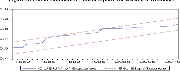
Figure-4: Plot of Cumulative Sum of Squares of Recursive Residuals
-0.4 0.0 0.4 0.8 1.2 1.6
1980 1985 1990 1995 2000 2005 2010
CUSUM of Squares 5% Significance
The straight lines represent critical bounds at 5% significance level.
Figure 4 and 5 belongs to the results of CUSUM and CUSUMSQ tests, respectively. The
graph of CUSUM test lies between the critical bounds (red lines) but graph of CUSUMsq test
does cross red lines at 5 per cent confidence interval. This indicates the instability of the
ranging in a linear fashion from zero at the first-ordered observation to one at the end of the sampling interval if
the null hypothesis is correct. In both the CUSUM and CUSUMSQ tests, the points at which the plots cross the
ARDL estimates. Parameter instability is found around 1996-97 in CUSUMsq test at 5 per
cent confidence interval. This structural break point is linked to efforts of Iranian government
to control inflation. In 1994 and 1995 Iran faced very high inflation. So that in 1996-1997
government tried to control the liquidity by controlling the banks credit.
We have also applied Chow forecast test to validate the significance of structural break in
Iran over the period of 1996-97. The results are reported in Table-7. It is pointed by Leow,
(2004) that Chow forecast is preferred over graphs. Graphs often provide ambiguous results.
The results in Table-7 indicate that forecast test accepts hypothesis of no structural change in
our model.
Table-7: Chow Forecast Test
Forecast from 1996 to 2011
F-statistic 0.2783 Probability 0.9923
Log likelihood ratio 8.1439 Probability 0.9178
The VECM Granger Causality Analysis
Once cointegration is found between the variables, we should apply the VECM Granger
causality approach to examine causal relationship between income inequality, financial
development, economic growth, inflation and globalization. It is also supported by Granger,
(1969) to apply the VECM Granger approach if variables are found to stationary at same
level. The direction of causal relationship between income inequality, financial development,
economic growth, inflation and globalization would help policy makers to equalize income
The results of the VECM Granger causality are reported in Table-8. It is found that the
estimates of ECMt1 have negative sign and statistically significant in all VECMs except in
financial development (lnFt) and globalization (lnGt) equations. It implies that shock
exposed by system converging to long run equilibrium path at a slow speed for income
inequality equation (-0.5228) and economic growth equation (-0.4780) VECMs as compared
to adjustment speed of inflation equation (-0.6477).
In long run, causal relationship reveals that feedback hypothesis is found between income
inequality and economic growth. This finding is contradictory with Risso and Carrera, (2012)
who reported unidirectional causality running from income inequality to economic growth in
pre-reforms and neutral hypothesis is found between both variables in post reforms in China.
But, Huang et al. (2011) reported that economic growth Granger causes regional income
inequality. Financial development Granger causes income inequality. This finding is
consistent with Gimet and Lagoarde‐Segot, (2011) who reported that financial sector plays its
vital in declining income inequality. The unidirectional causality running from financial
development to economic growth confirms the existence of supply-side hypothesis in case of
Iran. Our results have been supported by Shiva, (2001) who documented that financial
development plays a vital role to lead economic growth. The feedback effect is found
between inflation and income inequality. On contrary, Shahbaz et al. (2010) reported that
inflation improves income distribution through redistributive policies. Globalization Granger
causes income inequality. This view in contradictory to Mah (2002) who noted that
globalization leads to deteriorate income inequality in Korea but Mousavi and Taheri, (2008)
could not find a significant relationship between globalization and income distribution in case
of Iran.
Table-8: VECM Granger Causality Analysis
Dependent
Variable
Type of causality
Short Run Long Run
1
ln
IEt
lnYt1
lnFt1
lnINt1
lnGt1 ECTt1t
IE
ln
… 7.9826*
[0.0017]
1.2436
[0.3032]
1.6248
[0.2144]
1.0938
[0.3484]
-0.5228**
[-2.6066]
t
Y
ln
6.9088*
[0.0035]
… 1.4883
[0.2492]
2.8118***
[0.0765]
3.1763***
[0.0566]
-0.4780*
[-3.4499]
t
F
ln
0.7830
[0.4661]
2.8678***
[0.0725]
… 1.6603
[0.2071]
0.3132
[0.7735]
…
t
IN
ln
3.4047**
[0.0470]
1.2088
[0.3132]
2.3398
[0.1147]
… 0.0171
[0.9831]
-0.6477*
[-3.7251]
t
G
ln
0.6192
[0.5451]
2.8788***
[0.0718]
0.2836
[0.7550]
0.3811
[0.6863]
… …
Note: *, ** and *** represent significance at 1%, 5% and 10% levels respectively.
In short run, bidirectional causality exists between income inequality and economic growth.
The feedback effect is found between economic growth and globalization. The unidirectional
causal relationship is found running from income inequality to inflation. Economic growth
Granger causes financial development.
V: Conclusion and Policy Implications
In this study long-run and short-run relationship between financial development and income
inequality has been investigated in case of Iran. We have applied the ARDL bound testing
approach for long run and error correction model for short run dynamics. The structural break
unit root tests have applied to test the integrating order of all the variables.
Greenwood-Jovanovich, (1990) hypothesis which illustrates an inverted-U shape relationship between