Development of an Efficient Genetic Algorithm for the Time Dependent Vehicle Routing Problem with Time Windows

(1)

http://www.scirp.org/journal/ajor ISSN Online: 2160-8849

ISSN Print: 2160-8830

Development of an Efficient Genetic Algorithm

for the Time Dependent Vehicle Routing

Problem with Time Windows

Suresh Nanda Kumar, Ramasamy Panneerselvam

School of Management, Pondicherry University, Pondicherry, India

Abstract

This research considers the time-dependent vehicle routing problem (TDVRP). The time-dependent VRP does not assume constant speeds of the vehicles. The speeds of the vehicles vary during the various times of the day, based on the traffic conditions. During the periods of peak traffic hours, the vehicles travel at low speeds and during non-peak hours, the vehicles travel at higher speeds. A survey by TCI and IIM-C (2014) found that stoppage delay as per-centage of journey time varied between five percent and 25 percent, and was very much dependent on the characteristics of routes. Costs of delay were also estimated and found not to affect margins by significant amounts. This study aims to overcome such problems arising out of traffic congestions that lead to unnecessary delays and hence, loss in customers and thereby valuable reve-nues to a company. This study suggests alternative routes to minimize travel times and travel distance, assuming a congestion in traffic situation. In this study, an efficient GA-based algorithm has been developed for the TDVRP, to minimize the total distance travelled, minimize the total number of vehicles utilized and also suggest alternative routes for congestion avoidance. This study will help to overcome and minimize the negative effects due to heavy traffic congestions and delays in customer service. The proposed algorithm has been shown to be superior to another existing algorithm in terms of the total distance travelled and also the number of vehicles utilized. Also the per-formance of the proposed algorithm is as good as the mathematical model for small size problems.

Keywords

Time-Dependent Vehicle Routing Problem, Genetic Algorithm, Chromosomes, Cross-Over, Travel Times, Vehicles

How to cite this paper: Kumar, S.N. and Panneerselvam, R. (2017) Development of an Efficient Genetic Algorithm for the Time Dependent Vehicle Routing Problem with Time Windows. American Journal of Operations Research, 7, 1-25.

http://dx.doi.org/10.4236/ajor.2017.71001

Received: November 7, 2016 Accepted: December 24, 2016 Published: December 27, 2016

http://creativecommons.org/licenses/by/4.0/

(2)

1. Introduction

Vehicle travel times in the cities and urban areas vary due to various reasons and factors, like congestions in traffic, accidents, road repairs, movement of impor-tant personalities who need high security, and weather conditions. If these travel time variations are ignored during the process of developing route plans for pick-up and/or delivery vehicles, the development of route plans may be ineffi-cient in terms of the vehicles travelling into congested urban traffic conditions. Due to these travel time variations, in some cases the vehicles waste valuable time in traffic jams and customers have to wait unreasonably long without hav-ing any reliable information about the actual arrival times of vehicles. In these circumstances, it becomes difficult to satisfy the time windows during which the demand nodes must be visited.

In addition, insertion of new demands for pick-up that arise after completion of route planning, in the planned vehicle routes in real time, may result in sig-nificant savings. Considering time-dependent travel times as well as information regarding demands that arise in real time in solving vehicle routing problems can reduce the costs of ignoring the changing environment.

2. Literature Review

The basic VRP relies on the assumption that travel times remain constant throughout the whole planning horizon. In reality, however, travel times may vary during the day. The variation in travel times may result from predictable events such as congestion during rush hours or from unpredictable events such as accidents (Ichoua et al. [1]). The TDVRP takes these predictable events into account by assuming time-dependent travel times, i.e. the travel time between two locations depends on the distance between these two points and on the time of the day (Malandraki and Daskin [2]).

According to Ichoua et al. [1], the optimal solution of a VRP which assumes constant travel times, may be suboptimal or infeasible for the time-dependent problem. For example, time windows might be missed because of late arrivals, transportation costs might increase because of overtime hours, etc. The TDVRP captures this aspect by taking predictable travel time variations into account. The aim of the problem is to construct feasible routes which minimize the total travel time and offer a higher reliability.

(3)

Hence, the total time taken for travel between two locations is dependent on the specific departure time. Hence to take these external influences into consid-eration, the VRPTW is extended and is studied as time-dependent vehicle routing problem with time windows (TDVRP). The driving time that changes with the time of the day, is suitably represented by a time-dependent function.

Time-dependent travel times (or travel speeds) are either simulated or derived from traffic monitoring systems. When analyzing the data from traffic monitor-ing systems, one can observe that most travel times follow a certain pattern dur-ing the day. This helps to predict future traffic situations. Especially travel time variations during rush hour congestion show a high predictability. This is prov-en by Eglese et al. [3] who mention a study from the United Kingdom which examines speedometer analysis and data from a vehicle tracking and tracing sys-tem. It shows that on one road segment of a motorway, the same commercial vehicle speeds vary in one week from 5 mph (at 8:45 am on a Monday) to 55 mph (at 8:15 pm on a Wednesday). When comparing the observed speeds over a period of ten weeks, the variation in speed for the same time of a day and the day of a week is less than 5%. According to Eglese et al. [3], this small variation shows that travel speeds are highly predictable and can be forecasted for any road length and any time of the day.

2.1. Time-Dependency in Vehicle Routing Problem

The literature relating to the TDVRP is rather scarce when compared to other VRP variants. However, Ichoua et al. [1] mention three related time-dependent problems which have been extensively studied:

The first problem mentioned is the time-dependent shortest path problem which was introduced in the late 1950s (Ford and Fulkerson [4]). It belongs to the earliest models dealing with time-dependency. Marguier and Ceder [5] con-sider a time-dependent path choice problem. In this case, a set of passengers is distributed in a transportation network consisting of overlapping bus routes with common stops. The passenger waiting times are represented by time-dependent distributions. The last problem mentioned is the time-dependent trav-eling salesman problem (TSP) (Miller et al., [6]). The problem concerns the de-termination of a least-cost route which visits each city exactly once. The travel cost between each city is time-dependent.

2.2. Time-Dependent VRP (TDVRP)

(4)

to-tal route duration, the number of vehicles and transportation cost can be deter-mined. All TDVRP articles which have been studied satisfy the First-In First-Out (FIFO) property (Ichoua et al. [1]), which states that a vehicle that leaves earlier from some customer will arrive earlier at its destination. The time-dependent travel are modelled following the example of Ichoua et al. [1], where the work-day is partitioned into several periods and a constant travel speed is assigned to each time interval, resulting in speed being a step function of the departure time for all the arcs. The higher the number of time intervals, the more realistic the model will be because the travel speeds will change more gradually instead of abruptly (Kok et al. [7]). The travel time between two customers is then depen-dent on the departure time from the first customer and the time-dependepen-dent speed on the associated arc between the two customers.

2.3. Classification of Time-Dependent Models

According to Ichoua et al. [1], TDVRP models can be classified into four main categories based on the type of travel time function:

The first category refers to models based on simple travel time functions. In this case, multiplier factors are used to integrate time-dependency.

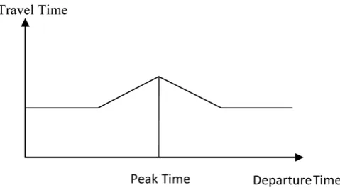
Other TDVRP models assume discrete travel times (Malandraki and Daskin

[2]). For this purpose, the time horizon is partitioned into discrete time intervals and the travel time is defined as a step function as in Figure 1, from the starting time as the origin node. As the travel time changes appear in the form of jumps, it might happen that the FIFO property is not satisfied if the travel time in a consecutive time interval decreases. The FIFO property guarantees that if two vehicles depart from the same origin node for the same destination node, the one which started earlier will also arrive earlier.

[image:4.595.254.494.570.704.2]

Ahn and Shin [12] investigated the effect of the first feasibility condition in an insertion heuristic and the effect of the third feasibility condition in the tour im-provement heuristic. In their study, they observed a substantial reduction in computation times when compared to the case where no feasibility conditions are implemented. Malandraki and Daskin [2] discuss a TDVRP with time win-dows. The objective is to minimize the total route time, consisting of the sum of

Figure 1. Travel time function with a single peak (Ahn and Shin

(5)

all travel times, service times and waiting times. The authors developed a model based on a mixed integer linear programming (MILP) formulation. The heuris-tics are tested on 32 randomly generated problems which consist of 10 to 25 customers.

Hill and Benton [13] proposed a model for the vehicle scheduling problems. This is formulated on the basis of intra-city time-dependent travel speeds. Their model consists of n nodes. This model does not satisfy the FIFO property as mentioned by Ichoua et al. [1]. They used a single vehicle and five locations. They solved this problem and published the results. They used a small set of historical travel time data and assumed 24 periods per day of 1 hour intervals.

Ichoua et al. [1] conducted research on the TDVRP. They presented a VRP based on time-dependent travel times and speeds. This problem has each cus-tomer associated with a soft time window [ei, li] and a service time. If the vehicle

arrives earlier, it results in a waiting time while a late arrival time will incur a penalty cost. The objective of the problem is to minimize the weighted sum of the total travel time and the total lateness over all customers. The authors de-velop a parallel tabu search heuristic with an adaptive memory based on the work of Taillard et al. [14]. Finally, the TDVRP is implemented in a dynamic setting where new customer demands occur during the day. To solve the dy-namic version, they used an algorithm based on the work of Gendreau et al. [15]

where vehicles are allowed to wait at their current location so that they can react to new requests in their vicinity. In this case, a departure time which prevents too early arrival at the next customer location needs to be determined.

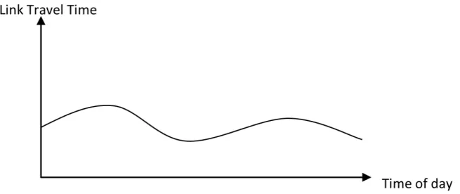
[image:5.595.212.540.579.717.2]

Fleischmann et al. [16] implemented the time-varying travel times in various vehicle routing algorithms with time windows. The travel time data is provided by the traffic information system LISB (Berlin). The most important work con-sidered in the literature of this study is the work done by Haghani and Jung [17]. They examined the dynamic VRP with time-dependent travel times, soft time windows and real-time vehicle control. In the problem, routes are adjusted at different times of the day. During each adjustment, new information about ve-hicle locations, travel times and demands is integrated into the model. The au-thors used a continuous travel time function where the slope is set to be less than one in case of a travel time decrease as shown in Figure 2.

(6)

Haghani and Jung [17] defined the VRP as a MILP problem. The objective is to minimize the total cost, consisting of the fixed vehicle costs, the routing costs and the penalties for time window violations. They developed a GA solution, a lower bound (LB) solution and an exact solution. These are based on a set of randomly generated test problems. The authors obtained exact solutions for up to ten customers and LB solutions for 15 to 30 customers. For problems with up to ten customers, they implemented 10 to 15 time intervals whereas for problems with 30 customers, they used 30 time intervals. They reported that the GA re-sults based on ten customers are similar to the exact rere-sults. The gaps between the GA results and the lower bounds are below 5% for all problems where the number of customers ranges between 5 and 25 (10 time intervals). Given the problem with 30 customers (30 time intervals), the gap amounts to 7.9%. Finally, they tested the GA in a simulated network where accidents cause significant congestion in certain parts of the road network. They compared a static and a dynamic approach. The dynamic approach allows the re-planning of routes based on real-time travel time information at regular intervals during the day. In this case, the travel speed of a link can be calculated at any time during the day. The authors concluded that the dynamic routing plan leads to better results than the static one especially if the traffic situation is very unstable.

Woensel et al. [18] presented a dynamic vehicle routing problem with time- dependent travel times by taking traffic congestion into consideration. This model which was developed by them is based on queuing models which capture the stochastic and dynamic aspects of travel time. They compared three different speed approaches. In the first case, they assumed constant travel speeds. In the second case, they modelled the travel time function by dividing the day into three time intervals, each corresponding to a different travel speed. In the third case, the day is divided into 10 minute-intervals where the associated travel speeds are based on queuing models. They used TS to solve the problem. For the sake of comparison, they recalculated the resulting solutions with a different va-lidation dataset for a different day. The authors then conducted tests based on the benchmark instances of Augerat et al. [19]. They established that the time- dependent case comprising of three time zones performs considerably better than the time-independent case. The authors hence concluded that when there is a high variability of travel speeds, it is best to take into account the time-dependent travel times to achieve efficient results. Moreover, the solution quality in-creases, when more time intervals and road types are considered.

(7)

Balseiro et al. [23] tested the performance of the TDVRP with time windows. First they developed a MACS algorithm hybridized with insertion heuristics (MACS-IH) based on the minimum delay technique (MDL). The aim is to create an insertion heuristic which leads to a higher number of feasible solutions. They formulated the problem as a MILP problem. They used the earlier formulation of Malandraki and Daskin [2] as a starting point. Vehicles are required to wait at the customer locations, to satisfy the time window constraint if they arrive too early. They divided the time horizon into M time intervals and the end of an in-terval is denoted Tm. A hierarchical objective is proposed, in which the primary

objective minimizes the number of vehicles whereas the secondary objective mi-nimizes the total time of all routes, consisting of all travel times, service times and waiting times. Furthermore, the authors performed tests with the time-dependent instances of Ichoua et al. [1].

Ehmke et al. [24] considered the TDTSP and the TDVRP. They used time- dependent travel times which are based on Floating Car Data (FCD) from Stutt-gart, Germany. These travel times are transformed into planning data sets through Data Mining procedures. They used two types of travel time planning sets: The first planning set is based on FCD averages which represent day-specific travel times derived from aggregating historical FCD to one average meas-ure per network segment and day of the week. The second planning set relies on FCD hourly averages which represent travel times derived from aggregating his-torical FCD to 24 averages per network segment, dependent on the day of the week and the time of the day. The authors examined two routing approaches, viz. the static routing approach which is based on the first travel time planning set whereas the time-dependent routing approach relies on the second travel time planning set. They used time-dependent distance matrices which are determined with shortest path algorithms. These algorithms are based on a time-dependent digital road map of the city road network which satisfies the FIFO property.

2.4. Summary of the Literature Review

In this section, the reviewed papers are summarised in the Table 1.

3. Mathematical Model and Algorithm Development

In this section, the mathematical model which is developed in this research to solve the TDVRP and the genetic algorithm for the TDVRP are discussed in de-tail. Usinga flow-arc formulation [Desrochers et al. [25]], TDVRPTW is de-scribed as follows. Let G = (V, A) be a graph where A = {(vi, vj): i ≠ j (for alli, j ∈

V) is an arc set and the vertex (node) set is V = (v0, …, vn+1). Vertices v0 and vn+1

denote the depot at which vehicles of capacity qmax are based. Each vertex in V

has an associated demand qi ≥ 0, a service time gi ≥ 0, and a service time window

[ei, li]; in particular the depot has g0 = 0 and q0 = 0. The set of vertices C =

{v1, …,vn} specifies a set of n customers. The arrival time of a vehicle at customer

i, is denoted ai and its departure time bi. Each arc (vi, vj) has an associated

(8)

Table 1. Overview of TDVRPTW articles.

Article Variant of TDVRP Objective (Min.) Solution method

Kuo et al.

(2009) TDVRP Total route duration Tabu search

Kok et al.

(2012) TDVRP with hard TW Total route duration

Dijkstra algorithm and restricted dynamic programming heuristic

Balseiro et al.

(2011) TDVRP with hard TW

First number of routes, second total

route duration

Ant colony algorithm with insertion heuristics

Figliozzi

(2012) TDVRP with hard and soft TW

First number of routes, second total

route duration Iterative route construction and improvement heuristic Hagani & Jung (2005)

Dynamic vehicle routing problem with time-dependent travel times

Total distance

travelled Genetic Algorithm

0 which is a function of the departure time from customer i. The set of available vehicles is denoted by K.

The cost per unit of route duration is denoted as Ct; the cost per unit distance

travelled is denoted Cd. It is assumed that the problem is feasible, i.e. it is always

feasible to serve any individual customer starting from the depot. The primary objective function for the TDVRP is the minimization of the number of routes or the number of vehicles utilized. The optimal number of routes is unknown. A secondary objective is the minimization of total time or distance travelled. There are two decision variables in this formulation; k

ij

x is a binary decision variable

that indicates whether vehicle k travels between customers i and j. The real number decision variable k

i

y indicates service start time for customer i served

by vehicle k.

3.1. Mathematical Model for TDVRPTW

The mathematical model of TDVRPTW is given as below.

0

min imize kj k K j C

x

∑∑

  (1)

( ),

(

1 0

)

0

min imize k k k k k ,

d ij ij t n j

k K i j A k K j C

C

∑ ∑

d x +C

∑∑

y+ −y x

    (2)

Subject to:

max,

k i ij i C j V

q x ≤q ∀k K

∑ ∑

 

 (3)

1, k ij i C j V

x = ∀i C

∑∑

 

 (4)

0, , k k

il ij i V i V

x − x = ∀i C ∀k K

∑

    (5)

0 0, 0, ,1,

k k

i n i

(9)

0 1,

k j j V

x = ∀k K

∑



 (7)

, 1 1,

k j n j V

x + = ∀k K

∑



 (8)

, , k k

i ij i j V

e

∑

x ≤ y ∀i C ∀k K 

  (9)

, , k k

i ij i j V

l

∑

x ≥ y ∀i C ∀k K 

  (10)

(

,

)

, , ,

( )

,

k k k k

ij i i i j i i j

x y +g +t y +g ≤y i C ∀ i j A ∀k K (11)

{ } ( )

0,1 , , , k

ij

x ∀ i j A ∀k K (12)

The objectives of the TDVRPTW are defined by (1) and (2) respectively. The constraints are defined as follows: the total demand in a particular route should not exceed the vehicle capacity (3); all the customers must be served and each customer must be served exactly once (4); a vehicle that arrives at a customer should also depart from that customer (5); routes must start at the depot and end at the depot (6); each vehicle leaves from the depot and returns to the depot exactly once, (7) and (8) respectively; service times must satisfy time window start (9) and ending (10) times specified; service start time must allow for travel time between customers (11). Decision variables type is indicated in (12).

During real-time traffic situations, the assumption of constant speed will not hold good. Hence we need to find out alternate routes, to minimize the distance travelled and the number of vehicles utilized as well as to minimize the total time taken to cover the entire tour. The problem lies in finding an efficient GA-based meta-heuristic which is more efficient than existing algorithms. A genetic algo-rithm to solve the TDVRP is developed. The problem that has been considered is a pick-up or delivery vehicle routing problem to various customers or from the various supplier sites with time windows in which we consider multiple vehicles with different capacities, with real-time variations in travel times between the different nodes. To load and start the time dependent VRP variant in Heuristic-Lab, we first need a valid file to load the time-dependent VRP data from. We use the data from the Solomon (CVRPTW) instances and add the travel time ma-trices. The dimension of the travel time matrix must match the number of cities. For the travel times, random values between 0.5 and 1.0 were generated using random function in Excel. The performance of the genetic algorithm for TDVRP is evaluated by comparing its results with one more existing algorithm for the TDVRPTW developed by Hashimoto et al. [26].

A modified version of the Genetic Algorithm formulation developed for the VRPTW solution developed by Nandakumar and Panneerselvam [27] has been used in this stud. This algorithm is described below.

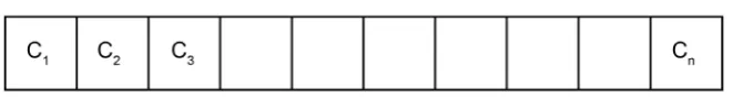
3.2. Chromosome Representation

(10)

[image:10.595.208.539.66.110.2]

Figure 3. Chromosome sample.

In the Figure 3, n is the total number of customers. Each chromosome con-sists of a set of genes. In the chromosome shown in the Figure 3, the genes c1,

c2, ···, cn are defined as Customer IDs/Nodes. Every chromosome is initialized as

the route which contains the source location and the destination location at the start and end of the array, respectively. Each chromosome is a solution path.

A crossover operator is a major process of producing offspring from the cur-rent population. There are many methods for crossover operation according to different problems. In this paper, “Random Sequence Insertion-Based Crossov-er” method is used, which is explained in the next section.

The Vehicle Routing Problem with Time Windows is solved using the Genetic Algorithm (GA) with multi-chromosome representation. It is used for finding a (near) optimal solution to a variation of the TDVRPTW by setting up a GA to search for the shortest route (distance), taking into account additional con-straints, and minimizing the number of vehicles used.

3.3. Genetic Algorithm (SNRPGA2)

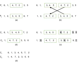
The steps of the proposed genetic algorithm (SNRPGA2) for the time dependent vehicle routing problem with time windows are presented below. A schematic view of the crossover operation used in this algorithm is shown in Figure 4.

The steps of the Random Sequence Insertion-based Crossover (RSIX) method are presented below.

Step 1: Two chromosomes from the chromosome pool are randomly chosen as parents.

Step 2: Generate two crossover points, which will lead to three chromosome segments in each chromosome as shown in Figure 4(a).

Step 3: Next, swapping operation of the middle crossover genes segment takes place, as in Figure 4(b).

Step 4: Next, taking into account the VRPTW constraints, with each customer (node) allowed to be visited only once, assuming that ∀

( )

i j, , d0i < d0j + dji

tri-angle property and accommodating time window constraint with possible wait-ing time, use the data from the Solomon (CVRPTW) and add the travel time matrices. For the travel times, random values between 0.5 and 1.0 have been generated. Then retain the gene segment that underwent crossover, and then remove the gene (node) with same value, in their parent chromosome, such as in

Figure 4(c).

Step 5: This results in obtaining two new offspring having gene segments that underwent crossover and they are added into the next generation as shown in

Figure 4(d).

• _{The new offspring are tested for fitness values.}

(11)

[image:11.595.212.534.58.317.2]

Figure 4. Crossover operation.

Mutation to Chromosomes

After the crossover is carried out on each chromosome, mutation operation is carried out to improve the chromosome. During the mutation operation, two randomly chosen genes are selected and the mutation operator changes their value into other possible values. Mutation helps to prevent the genetic algorithm from converging to local optima. Other genetic algorithms parameters can also influence the GA efficiency. Crossover probability which is specified in the GA, determines the rate at which the crossover occurs. Mutation probability that is specified is used to find how often the mutation is applied on the offspring. If no mutation happens, the respective chromosome is replaced in the population without any change. The population size defines the number of individuals in the population. The results of application of the mutation operation on the offspring shown in the Figure 4(d) are shown in Figure 5.

3.4. Evaluation of Fitness Function

According to Sivasankaran and Sahabudeen [28], the fitness function of the chromosome is obtained by assigning the nodes serially from left to right from its ordered vector into customer IDs or nodes for a given travel route. This idea is used in this research to find the fitness function value of each chromosome/ offspring. Every road or route chromosome (offspring) has its own fitness value, which is obtained by adding the distances between the consecutive pairs of the nodes (genes) in it and the distance between the last node (gene) in it and the first node (gene) in it.

(12)

[image:12.595.210.536.74.217.2]

Figure 5. (a) Mutation of offspring 1; (b) Mutation of offspring 2.

function value are as listed below.

1) Each vehicle starts at the depot or warehouse, travels to a set of customer nodes and ends at the depot.

2) Except for the depot, each customer node is visited exactly once by the ve-hicle.

3) This algorithm uses a special, multiple-chromosome (parents) genetic re-presentation to code solutions into individual offspring, which offer better routes and solutions.

4) Special genetic operators like selection, crossover and mutation are used. 5) The number of vehicles used is minimized using this algorithm.

6) Additional constraints have to be satisfied. Minimum number of vehicles to cover all the nodes.

Minimizing the maximum distance travelled by each vehicle.

7) Time windows are defined for each customer node (e.g. unloading/loading times) and time-dependent travel times are introduced, by using a travel time matrix.

8) The single route chromosome is then assigned to multiple sub chromo-somes of smaller routes consisting of a set of customers from the original chro-mosome. Each route is assigned a vehicle to visit each customer node on the route to meet the customer’s demand in the route.

The variables used are the number of vehicles, the number of customers to be serviced by the vehicles, vehicle capacities, maximum distance travelled by each vehicle which is to be minimized. The objective is to minimize the number of vehicles used and the total distance travelled by the vehicles, in servicing the customers. The time of the day during which the vehicles are sent to the supplier sites for the pick-ups is also considered in this research.

3.5. Genetic Algorithm (SNRPGA2)

The steps of the proposed genetic algorithm (SNRPGA2) for the time dependent vehicle routing problem with time windows are presented below.

Step 1: Input the following:

(13)

Number of vehicles (k) Capacity of the vehicles (a) Set Generation Count (GC) = 1

Maximum number of generations to be carried out (MNG) = 1000 Step 2: Generate a random initial population (L) of 100 (N) chromosomes (suitable solutions routes for the problem).

Step 3: Evaluate the fitness function f(x) of each chromosome in the popula-tion L.

Step 4: Selection.

Sort the population L by the objective function (fitness function) value in the ascending order, since the objective of the study is minimization of the total dis-tance travelled. Copy a top 30% of the population to form a subpopulation S rounded to the whole number. Smaller fitness value is preferred here.

Step 5: Randomly select any two unselected parent chromosomes from the subpopulation S. Let them be c1 and c2 using tournament selection.

Step 5.1: Perform two-point random Cross-Over using the random sequence insertion-based crossover (RSIX) for the TDVRPTW described in the earlier section among the chromosomes c1 and c2 to obtain their offspring d1 and d2 by

assuming a crossover probability of 0.7.

Step 5.2: Perform mutation on each of the offspring using a mutation proba-bility of 0.3.

Step 5.3: Evaluate the fitness function with respect to the total distance tra-velled and number of vehicles utilized value for each of the offspring d1 and d2.

Step 5.4: Replace the parent chromosomes c1 and c2 in the population with the

offspring d1 and d2, respectively, if the fitness function of the offspring is less

than that of the parent chromosomes.

Step 6: Increment the generation count (GC) by 1 i.e., GC = GC + 1

Step 7: If GC ≤ MNG, then go to step 4, else go to step 8.

Step 8: The topmost chromosome in the last population serves as the solution for implementation.

Print the tour along with the total distance travelled and number of vehicles used.

Step 9: Stop.

4. Results

In this section a detailed presentation of the experimental results is given, for the time-dependent vehicle routing problem (TDVRP).

4.1. Comparisons of Algorithms in Terms of Number of Vehicles Utilized

(14)

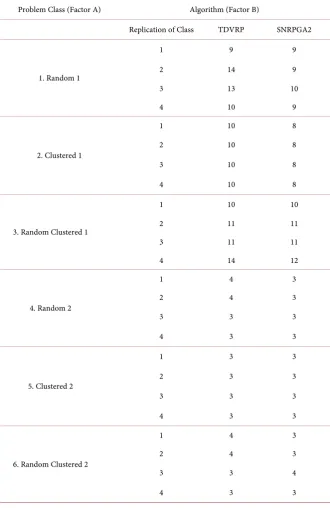
iterated local search algorithm proposed by Hashimoto et al. [26]. The number of factors in the experiment is 2, viz. Factor A (Problem Size) and Factor B (Al-gorithm). The number of levels for the Factor A is 6, Random 1, Clustered 1, Random Clustered 1, Random 2, Clustered 2 and Random Clustered 2, and that for the Factor B is 2, viz. TDVRPTW and SNRPGA. The results in terms of the number of vehicles utilized as per this design are shown in Table 2.

The model of ANOVA is given as below:

ijk i j ij ijk

[image:14.595.207.538.232.741.2]

Y = +µ A +B +AB +e

Table 2. Results of number of vehicles utilized.

Problem Class (Factor A) Algorithm (Factor B)

Replication of Class TDVRP SNRPGA2

1. Random 1

1 9 9

2 14 9

3 13 10

4 10 9

2. Clustered 1

1 10 8

2 10 8

3 10 8

4 10 8

3. Random Clustered 1

1 10 10

2 11 11

3 11 11

4 14 12

4. Random 2

1 4 3

2 4 3

3 3 3

4 3 3

5. Clustered 2

1 3 3

2 3 3

3 3 3

4 3 3

6. Random Clustered 2

1 4 3

2 4 3

3 3 4

(15)

where,

Yijk is the number of vehicles utilized w.r.t the kth replication under the ith

treatment of factor A (Problem Size) and the jth_{treatment of factor B}

(Algo-rithm).

µ is the overall mean of the response variable.

Ai is the effect of the ith treatment of factor A (Problem Size) on the response

variable.

Bj is the effect of the jth treatment of factor B (Algorithm) on the response

va-riable.

ABij is the interaction effect of the ith Problem Size and jth Algorithm on the

response variable.

eijk is the random error associated with the kth replication under the ith

Prob-lem Size and the jth_Algorithm.

In this model, Factor A (Problem Size/Problem Class) is a random factor and the Factor B (algorithm) is a fixed factor. Since the factor A is a random factor, the interaction factor ABij is also a random factor. The replications are always

random and the number of replications under each experimental combination is 4. The derivation of the expected mean square (EMS) is given in Panneerselvam

[29]. To test the effect of Ai as well as ABij, the respective F ratio is formed by

di-viding the mean sum of squares of the respective component (Ai or ABij), by the

mean sum of squares of error. The F ratio of the component Bj is formed by

di-viding its mean sum of squares by the mean sum of squares of ABij

The alternative hypotheses of the model are as given below.

H1: There are significant differences between the different pairs of treatments

of Factor A (Problem Size) in terms of the number of vehicles utilized

of Factor B (Algorithm) in terms of the number of vehicles utilized.

H1: There are significant differences between the different pairs of interaction

between Factor A and Factor B in terms of number of vehicles utilized.

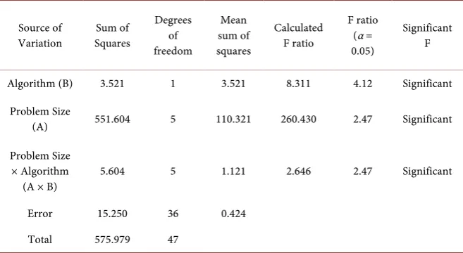
[image:15.595.209.538.553.733.2]

The results of ANOVA of the data given in the Table 2 are shown in Table 3.

Table 3. Analysis of variance for number of vehicles utilized.

Source of

Variation Squares Sum of

Degrees of freedom

Mean sum of squares

Calculated F ratio

F ratio (α = 0.05)

Significant F

Algorithm (B) 3.521 1 3.521 8.311 4.12 Significant

Problem Size

(A) 551.604 5 110.321 260.430 2.47 Significant

Problem Size × Algorithm

(A × B) 5.604 5 1.121 2.646 2.47 Significant

Error 15.250 36 0.424

(16)

From the ANOVA results shown in Table 3, one can infer that the factors “Problem Size”, “Algorithm” and “Interaction of “Problem size” and “Algo-rithm” have significant effects on the response variable “Number of Vehicles Utilized”. Since there are significant differences among the algorithms, the best algorithm is obtained using Duncan’s multiple range test by arranging the algo-rithms in the descending order of their mean total vehicles utilized, from left to right.

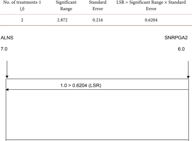
The standard error used in this test is computed as shown below using the mean sum of squares of the interaction terms (Problem Size × Algorithm) and the number of replications under each of the algorithms (24).

(

)

0.5

(

)

0.5

MSSAB 1.121 24 0.216

SE= ÷n = ÷ =

The least significant ranges (LSR) are calculated from the significant ranges of Duncan’s multiple range tests table for α = 0.05 and 36 degrees of freedom as shown in Table 4. The results of Duncan’s multiple range test are shown in Fig-ure 6 In this figure, the algorithms are arranged as per the descending order of their mean number of vehicles utilized from left to right. From this Figure 6, it is clear that there is a significant difference between the 2 algorithms in terms of the mean number of vehicles utilized and further the proposed algorithm SNRPGA2 utilizes the minimum mean number of vehicles compared to the oth-er algorithm.

4.2. Comparison of Algorithms in Terms of Total Distance Travelled

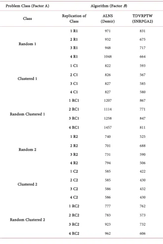
[image:16.595.211.537.474.713.2]

The proposed GA-based meta-heuristic for the time-dependent vehicle routing

Table 4. Duncan’s multiple range tests.

No. of treatments-1 (j)

Significant Range

Standard Error

LSR = Significant Range × Standard Error

2 2.872 0.216 0.6204

(17)

problem with time windows (SNRPGA2) is compared with one other existing meta-heuristics, viz. the algorithm developed for the TDVRPTW by Demir [30]

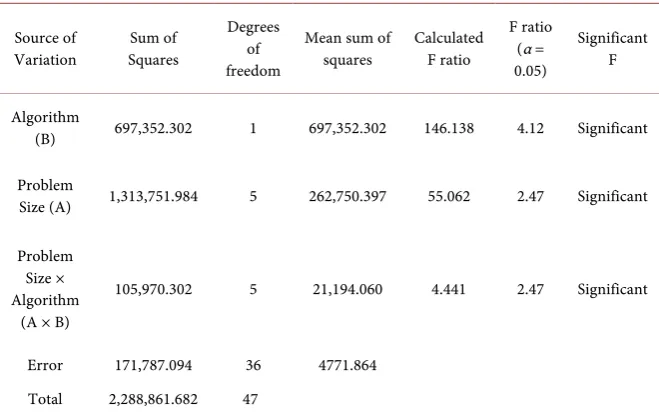
[image:17.595.207.538.254.747.2]

in terms of total distance travelled using a complete factorial experiment with two factors, viz. “Problem Size” and “Algorithm”. The number of levels for the problem size is 6, viz. C1, C2, R1, R2, RC1, RC2 from Solomon’s benchmark in-stances. The number of levels for “Algorithm” is 3 as already stated above. The number of replication under each experimental combination is 4. The results of the factorial experiment in terms of the total distance travelled are shown in Ta-ble 5. The application of ANOVA to the data given in Table 5 gives the results as shown in Table 6.

Table 5. Results of the factorial experiment in terms of the total distance travelled.

Problem Class (Factor A) Algorithm (Factor B)

Class Replication of _Class _(Demir)ALNS _(SNRPGA2)TDVRPTW

Random 1

1 R1 971 831

2 R1 932 675

3 R1 948 717

4 R1 1048 664

Clustered 1

1 C1 822 593

2 C1 826 567

3 C1 827 585

4 C1 827 580

Random Clustered 1

1 RC1 1207 867

2 RC1 1114 771

3 RC1 1258 847

4 RC1 1457 811

Random 2

1 R2 740 525

2 R2 701 688

3 R2 731 590

4 R2 794 506

Clustered 2

1 C2 585 422

2 C2 585 430

3 C2 586 432

4 C2 586 430

Random Clustered 2

1 RC2 777 762

2 RC2 783 573

3 RC2 923 732

(18)

[image:18.595.208.538.88.296.2]

Table 6. ANOVA for the total distance travelled.

Source of

Variation Squares Sum of

Degrees of freedom

Mean sum of

squares Calculated F ratio

F ratio (α = 0.05)

Significant F

Algorithm

(B) 697,352.302 1 697,352.302 146.138 4.12 Significant

Problem

Size (A) 1,313,751.984 5 262,750.397 55.062 2.47 Significant

Problem Size × Algorithm

(A × B)

105,970.302 5 21,194.060 4.441 2.47 Significant

Error 171,787.094 36 4771.864

Total 2,288,861.682 47

ijk i j ij ijk

Y = +µ A +B +AB +e

where,

Yijk is the total distance travelled w.r.t the kth replication under the ith

treat-ment of factor A (Problem Size) and the jth_{treatment of factor B (Algorithm).}

µ is the overall mean of the response variable total distance travelled

va-riable.

response variable.

In this model, the factor A is a random factor and the factor B is a fixed factor. Since the factor A is a random factor, the interaction factor is also a random factor. The replications are always random and the number of replications under each experimental combination is k. The derivation of the expected mean square (EMS) is given in Panneerselvam [29]. To test the effect of Ai as well as ABij the

respective F ratio is formed by dividing the mean sum of squares of the respec-tive component (Ai or ABij), by the mean sum of squares of error. The F ratio of

the component Bj is formed by dividing its mean sum of squares by the mean

sum of squares of ABij.

The alternative hypothesis of the model is stated as below:

of Factor A (Problem Size) in terms of the total distance travelled.

(19)

between Factor A and Factor B in terms of total distance travelled.

From the ANOVA results shown in Table 6, one can infer that the factors “Algorithm” and “Problem Size” have significant effects on the total distance travelled. Since, there is a significant difference among the 2 algorithms com-pared in terms of the total distance travelled, Duncan’s multiple range test is next conducted to identify the best algorithm by arranging the algorithms in the descending order of their mean total distance travelled from to right.

The standard error used in this test is computed as shown below using the mean sum of squares of the interaction terms (Problem Size × Algorithm) and the number of replications under each of the algorithms (24). The treatment means for the Factor B (Algorithm) in terms of the total distance travelled are arranged in the descending order from left to right. The standard error for the performance measure is calculated using the formula and found to be 22.92 One can notice the fact that the mean sum of squares of the interaction term AB is used in estimating the standard error (SE), because the F ratio for the factor “Algorithm” is obtained by dividing its mean sum of squares by the mean sum of squares of the interaction term ABij (Panneerselvam [29]).

The least significant ranges (LSR) are calculated from the significant ranges of Duncan’s multiple range tests table for α = 0.05 and 5 degrees of freedom as shown in Table 7.

(

)

0.5

(

)

0.5

MSS_AB 21194.060 24 29.72

SE= ÷n = ÷ =

[image:19.595.209.539.482.714.2]

From the Duncan’s Multiple Range Test performed above as shown in Figure 7, it is also clear that the TDVRPTW is superior in performance when compared

Table 7. Duncan’s multiple range tests.

No. of treatments-1

(j) Significant Range Standard Error LSR = Significant Range × Standard Error

2 2.872 29.72 85.356

(20)

to the existing algorithm based on ALNS used in this study for comparison, in terms of total distance travelled.

4.3. Comparison with the Mathematical Model

In this section a comparison is done between the proposed algorithm SNRPGA2 for the TDVRP and the mathematical model for the TDVRP for the two meas-ures, distance travelled and the number of vehicles used, which was solved using LINGO 15.0 optimization software.

A full factorial design is conducted for the comparison of the proposed GA- based algorithm, SNRPGA2 for the TDVRPTW with the mathematical model for the total distance travelled, whose data is given in Table 8. The experiment is conducted for small sized problems with six different levels of problem sizes starting from 10 nodes and then increasing the nodes in steps of 5 up to 35. The number of replications under each experimental combination is 2.

ijk i j ij ijk

Y = +µ A +B +AB +e

where,

Yijk is the total distance travelled w.r.t the kth replication under the ith

treat-ment of factor A (Problem Size) and the jth_{treatment of factor B (Algorithm).}

µ is the overall mean of the response variable total distance travelled.

variable.

[image:20.595.208.540.480.734.2]

va-riable.

Table 8. Comparison of the SNRPGA2 with the mathematical model for distance

tra-velled.

Problem Size (Number of

Nodes)

Replication Problem _instance

Method

SNRPGA2 Mathematical _Model

10 1 C102 35.754 35.754

2 C103 35.754 35.754

15 1 C102 87.815 87.815

2 C103 84.608 84.6079

20 1 C102 113.684 113.67

2 C103 103.55 103.50

25 1 C102 132.181 132.179

2 C103 124.45 124.44

30 1 C102 142.9 142.89

2 C103 135.171 135.161

35 1 C102 207.848 207.82

(21)

response variable.

In this model, the factor A is a random factor and the factor B is a fixed factor. Since the factor A is a random factor, the interaction factor is also a random factor. The replications are always random and the number of replications.

The alternative hypothesis of the model is stated as below:

of Factor A (Problem Size) in terms of the total distance travelled.

of Factor B (Algorithm) in terms of the total distance travelled.

between Factor A and Factor B in terms of total distance travelled. The ANOVA results are shown in the Table 9.

From the ANOVA results in Table 9 it is clear that there is no significant dif-ference between the proposed GA-based solution and the mathematical mod-el-based solution in terms of the total distance travelled.

Once again a full factorial design is conducted for the comparison of the pro-posed GA-based algorithm, SNRPGA2 for the TDVRPTW with the mathemati-cal model for the number of vehicles used, whose data is given in Table 10. The experiment is conducted for small sized problems with six different problem sizes starting from 10 nodes and then increasing the nodes in steps of 5 till 35 nodes. The number of replications under each experimental combination is 2.

[image:21.595.208.538.545.731.2]

From the Table 10, it is clear that the proposed algorithm (SNRPGA2) and the mathematical model give the same result in terms of number of vehicles used for the TDVRPTW problem for each replication under each of the problem sizes, which come under small/ medium size. Hence, there is no need of ANOVA for this comparison.

Table 9. ANOVA for the total distance travelled.

Source of

Variation Squares Sum of Degrees of freedom

Mean sum of squares

Calculated F ratio

F ratio (α =

0.05) Sig.

Problem

Size (A) 59,325.510 5 11,865.102 237.658 3.11 Significant

Algorithm (B) 0.021 1 0.021 0.000 4.75 Insignificant

Algorithm * Size

(AB) 0.073 5 0.015 0.000 3.11 Insignificant

Error 599.102 12 49.925

(22)

[image:22.595.205.538.102.379.2]

Table 10. Comparison of the SNRPGA2 with the mathematical model for the number of vehicles used.

Problem Size (Number of

Nodes) Replication

Problem instance

Method

SNRPGA2 Mathematical

Model

10 1 C102 1 1

2 C103 1 1

15 1 C102 2 2

2 C103 2 2

20 1 C102 2 2

2 C103 2 2

25 1 C102 3 3

2 C103 3 3

30 1 C102 3 3

2 C103 3 3

35 1 C102 4 4

2 C103 4 4

5. Conclusions

In this research, a GA based meta-heuristic is developed using Random Se-quence-based Insertion Crossover (RSIX) method (SNRPGA) for solving the time dependent vehicle routing problem (TDVRP) with time windows. Next, through a full factorial experiment with two factors, viz. “Problem Size” and “Algorithm”, it is proved that there are significant differences among the algo-rithms in terms of number of vehicles utilized (Kumar and Panneerselvam [29]). So, in the next stage using Duncan’s multiple range test, it is found that the pro-posed algorithm “SNRPGA2” is better than one more existing algorithm in terms of minimizing the number of vehicles utilized. Next, through another fac-torial experiment with two factors, viz. “Problem Size” and “Algorithm”, it is proved that there are significant differences among the algorithms in terms of the total distance travelled. So, in the next stage using Duncan’s multiple range test, it is found that the proposed algorithm “SNRPGA2” is better than the other existing algorithms in terms of minimizing the total distance travelled.

The proposed genetic algorithm is compared with the mathematical model and it is found that there is no significant difference in the results obtained by using the proposed GA and the mathematical model, in terms of each of the performance measures, viz. the number of vehicles used and the total distance travelled.

(23)

pe-riods of the day with time window requirements of the suppliers. Future re-searchers can implement the TDVRP using other meta-heuristics and compare the efficiencies of the various meta-heuristics. The Solomon’s benchmark in-stances are got from SINTEF [31].

References

[1] Ichoua, S., Gendreau, M. and Potvin, J.Y. (2003) Vehicle Dispatching with Time- Dependent Travel Times. European Journal of Operational Research, 144, 379-396. https://doi.org/10.1016/S0377-2217(02)00147-9

[2] Malandraki, C. and Daskin, M.S. (1992) Time-Dependent Vehicle-Routing Prob-lems: Formulations, Properties and Heuristic Algorithms. Transportation Science, 26, 185-200. https://doi.org/10.1287/trsc.26.3.185

[3] Eglese, R., Maden, W. and Slater, A. (2006) A Road Timetable to Aid Vehicle Routing and Scheduling. Computers and Operations Research, 33, 3508-3519. https://doi.org/10.1016/j.cor.2005.03.029

[4] Ford, J.L.R. and Fulkerson, D.R. (1956) Maximal Flow through a Network. Cana-dian Journal of Mathematics, 8, 399-404. https://doi.org/10.4153/CJM-1956-045-5 [5] Marguier, P. and Cedar, A. (1984) Passenger Waiting Strategies for Overlapping

Bus Routes. Transportation Science, 18, 207-230. https://doi.org/10.1287/trsc.18.3.207

[6] Miller, C.E., Tucker, A.W. and Zemlin, R.A. (1960) Integer Programming Formula-tions and Traveling Salesman Problems. Journal of the Association for Computing Machinery, 7, 326-329. https://doi.org/10.1145/321043.321046

[7] Kok, A.L., Hans, E.W. and Schutten, J.M.J. (2011) Optimizing Departure Times in Vehicle Routes. European Journal of Operational Research, 210, 579-587.

https://doi.org/10.1016/j.ejor.2010.10.017

[8] Li, H. and Lim, A. (2001) A Metaheuristic for the Pickup and Delivery Problem with Time Windows. IEEE Proceedings of the 13th International Conference on Tools with Artificial Intelligence, Dallas, 7-9 November 2001, 160-167.

https://doi.org/10.1109/ictai.2001.974461

[9] Lei, H., Laporte, G. and Guo, B. (2011) The Capacitated Vehicle Routing Problem with Stochastic Demands and Time Windows. Computers & Operations Research, 38, 1775-1783. https://doi.org/10.1016/j.cor.2011.02.007

[10] Figliozzi, M.A. (2009) A Route Improvement Algorithm for the Vehicle Routing Problem with Time Dependent Travel Times. Proceedings of the 88th Transporta-tion Research Board Annual Meeting, Washington DC, 11-15 January 2009, 616- 636.

[11] Kuo, Y., Wang, C.-C. and Chuang, P.-Y. (2009) Optimizing Goods Assignment and the Vehicle Routing Problem with Time-Dependent Travel Speeds. Computers and Industrial Engineering, 57, 1385-1392. https://doi.org/10.1016/j.cie.2009.07.006 [12] Shin Ahn, B.-H. and Shin, J.Y. (1991) Vehicle-Routing with Time Windows and

Time-Varying Congestion. Journal of the Operational Research Society, 42, 393- 400. https://doi.org/10.1057/jors.1991.81

[13] Hill, A.V. and Benton, W.C. (1992) Modelling Intra-City Time-Dependent Travel Speeds for Vehicle Scheduling Problems. Journal of the Operational Research So-ciety, 43, 343-351. https://doi.org/10.1057/jors.1992.49

(24)

portation Science, 31, 170-186. https://doi.org/10.1287/trsc.31.2.170

[15] Gendreau, M., Laporte, G. and Potvin, J.-Y. (2002) Metaheuristics for the VRP. In: Toth, P. and Vigo, D., Eds., The Vehicle Routing Problem (Monographs on Discrete Mathematics and Applications), SIAM, Philadelphia, 129-154.

[16] Fleischmann, B., Gietz, M. and Gnutzmann, S. (2004) Time-Varying Travel Times in Vehicle Routing. Transportation Science, 38, 160-173.

https://doi.org/10.1287/trsc.1030.0062

[17] Haghani, A. and Jung, S. (2005) A Dynamic Vehicle Routing Problem with Time-Dependent Travel Times. Computers & Operations Research, 32, 2959-2986. https://doi.org/10.1016/j.cor.2004.04.013

[18] Woensel, T.V., Kerbache, L., Peremans, H. and Vandaele, N. (2008) Vehicle Routing with Dynamic Travel Times: A Queueing Approach. European Journal of Operational Research, 186, 990-1007. https://doi.org/10.1016/j.ejor.2007.03.012 [19] Augerat, P., Belenguer, J., Benavent, E., Corber’an, A., Naddef, D. and Rinaldi, G.

(1995) Computational Results with a Branch and Cut Code for the Capacitated Ve-hicle Routing Problem. Technical Report 949-M, Université Joseph Fourier, Gre-noble.

[20] Maden, W., Eglese, R. and Black, D. (2010) Vehicle Routing and Scheduling with Time-Varying Data: A Case Study. Journal of the Operational Research Society, 61, 515-522. https://doi.org/10.1057/jors.2009.116

[21] Potvin, J.-Y. and Rousseau, J.-M. (1995) An Exchange Heuristic for Routeing Prob-lems with Time Windows. Journal of the Operational Research Society, 46, 1433- 1446.

[22] Solomon, M. (1987) Algorithms for the Vehicle Routing and Scheduling Problem with Time Window Constraints. Operations Research, 35, 254-265.

https://doi.org/10.1287/opre.35.2.254

[23] Balseiro, S.R., Loiseau, I. and Ramonet, J. (2011) An Ant Colony Algorithm Hybri-dized with Insertion Heuristics for the Time Dependent Vehicle Routing Problem with Time Windows. Computers & Operations Research, 38, 954-966.

https://doi.org/10.1016/j.cor.2010.10.011

[24] Ehmke, S., Meisel, S. and Engelmann, D.C. (2009) Mattfeld Data Chain Manage-ment for Planning in City Logistics. International Journal of Data Mining, Model-ling and Management, 1, 335-356.https://doi.org/10.1504/IJDMMM.2009.029030 [25] Desrochers, M., Lenstra, J.K., Savelsbergh, M.W.P. and Soumis, F. (1988) Vehicle

Routing with Time Windows: Optimization and Approximation. Vehicle Routing:

Methods and Studies, 16, 65-84.

[26] Hashimoto, H., Ibaraki, T., Imahori, S. and Yagiura, M. (2006) The Vehicle Routing Problem with Flexible Time Windows and Travelling Times. Discrete Applied Ma-thematics, 154, 2271-2290. https://doi.org/10.1016/j.dam.2006.04.009

[27] Kumar, S.N. and Panneerselvam, R. (2015) A Comparative Study of Proposed Ge-netic Algorithm-Based Solution with Other Algorithms for Time-Dependent Ve-hicle Routing Problem with Time Windows for E-Commerce Supply Chain. Journal of Service Science and Management, 8, 844-859.

https://doi.org/10.4236/jssm.2015.86085

[28] Sivasankaran, P. and Shahabudeen, P. (2013) Genetic Algorithm for Concurrent Balancing of Mixed-Model Assembly Lines with Original Task Times of Models.

Intelligent Information Management, 5, 84-92.

(25)

[30] Demir, E. (2012) Models and Algorithms for the Pollution-Routing Problem and Its Variations. PhD Thesis, University of Southampton, Southampton.

[31] SINTEF. Solomon’s Benchmark Instances.

https://www.sintef.no/projectweb/top/vrptw/solomon-benchmark/

Submit or recommend next manuscript to SCIRP and we will provide best service for you:

Accepting pre-submission inquiries through Email, Facebook, LinkedIn, Twitter, etc. A wide selection of journals (inclusive of 9 subjects, more than 200 journals)

Providing 24-hour high-quality service User-friendly online submission system Fair and swift peer-review system

Efficient typesetting and proofreading procedure

Display of the result of downloads and visits, as well as the number of cited articles Maximum dissemination of your research work

Submit your manuscript at: http://papersubmission.scirp.org/