Does oil price matter for Indian stock markets?

Munich Personal RePEc Archive

Does Oil Price Matter for Indian Stock

Markets?

Chittedi, Krishnareddy

Centre for Development Studies (Jawaharlal Nehru University),

India

2 November 2011

Online at

https://mpra.ub.uni-muenchen.de/35334/

DOES OIL PRICE MATTERS FOR INDIAN STOCK

MARKETS?

AN EMPIRICAL ANALYSIS

Krishna Reddy Chittedi Doctoral Scholar,

Abstract

This paper investigates the long run relationship between oil prices and stock prices for India over the period April 2000- June 2011. We employ Auto Regressive Distributed Lag (ARDL) Model that takes into consideration the long run relationship. The results obtained suggest that volatility of stock prices in India have a significant impact on the volatility of oil prices. But a change in the oil prices does not have impact on stock prices.

JEL classification: G12; O57

I Introduction

Changes in the price of crude oil are often considered an important factor for

understanding fluctuations in stock prices. In the long-term, the influence of oil

price on stock prices prevail, as oil price effect transmits to macroeconomic

indicators that influence liquidity of these markets. This suggests that the effect of

oil price changes transmit to fundamental macroeconomic indicators, which in turn

affect the long-term equilibrium linkage between these markets. Conditions that

reflect change in observable factors that affect an economy. Second, there are

speculative factors that operate entirely within a market over short periods. These

two sets of conditions sometimes work together, and sometimes opposite. Thus, a

given market can be speculatively strong, but fundamentally weak, or the reverse

Ravichandran (2010).

On theoretical grounds, oil-price shocks affect stock market returns or prices through

their effect on expected earnings (Jones et al., 2004).One rational of using oil price

change as a measure for change in key macroeconomic indicators is that value of stock

prices in theory equals discounted expectation of future cash flows (dividends), which

in turn are affected by macroeconomic events that possibly can be influenced by oil

shocks. Since oil price increase, it raises the production cost in industrial oil consuming

countries. Due to increase Oil price it is expected to raise the cost of imported capital

goods, therefore it may adversely affecting the prospects of higher profits for firms

traded in Indian stock markets. On the demand side, oil price increases drive up the

general level of prices, which translates into lower real disposable income, and

consequently reduces demand. Besides the direct impact on general price levels, oil

prices also have secondary effects on wage levels, which in combination with high

general prices result in increased inflation. Inflationary pressures are usually controlled

by central banks through increase in interest rates. Given the higher interest rates, bond

investments will become more attractive than stock investments, which will result in

lower stock prices. Finally, increasing import prices trigger a deterioration of the terms

of trade and therefore impose welfare losses. Oil-exporting countries, on the other

global oil demand (Bhar and Nikolova 2009). Liberalization and integration of

international markets economies (Chittedi 2010, 2011), characterised with increased

level of capital flows and international investments in emerging have made global

investors more vulnerable to oil price impact on emerging stock markets. Therefore,

understanding the level of susceptibility of stock prices in emerging economies to

movement in global oil prices is very important.

The remainder of the paper is organised as follows: Section 2 provides review of

previous studies on the study topic; Section 3 presents nature of data and the

methodology; Section 4 covers the discussion of the results; and Section 5 provides the

conclusions of the study.

II Review of Literature

There have been a large number of studies stating relationship between oil prices and

stock return. Most of these studies have reported significant effects of oil price changes

on stock return. For example, Adorsky (1999), Papapetrou (2001), Ciner (2001), Yang

and Bessler (2004), Anoru and Mustafa (2007), Kilian (2008) and Miller and Ratti (2009)

have investigated the effects of oil prices on stock prices in developed countries. In

addition, studies by Maghyereh (2004), Onour (2007), Aliyu (2009), and Narayan and

Narayan (2010) assessed the relationship between oil prices and Vietnam‟s stock prices

with daily series from 2000 to 2008. Using the Johansen test, the findings provided

evidence of oil prices, stock prices, and exchange rates for Vietnam sharing a long-run

relationship. In addition, the study found both oil prices and exchange rates have a

positive and statistically significant effect on Vietnam‟s stock prices in the long-run and

not in the short-run.

Bashar (2006) uses VAR analysis to study the effect of oil price changes on GCC stock

markets and shows that only the Saudi and Omani markets have predictive power of

oil price increase. Jones and Kaul (1996) examined the reaction of stock returns in four

developed markets (Canada, Japan, the UK, and the US) to oil price fluctuations on the

basis of the standard cash flow dividend valuation model. The study found that for the

US and Canada stock market reaction can be accounted entirely because of impact of

oil shocks on cash flows. However, some studies have shown that the link between oil

increases) tend to have larger impact on growth than positive shocks do [Hamilton

(2003), Zhang (2008), and Cologni and Manera (2009)]. Thus, we should expect that oil

prices equally affect stock markets in a nonlinear fashion.

Notwithstanding such widely held views in the financial press, there is no consensus

about the relation between the price of oil and stock prices among economists. Chen,

Roll and Ross (1986), for example, concluded that oil price changes have no effect on

asset pricing. Huang et al. (1996) provide evidence in favor of causality effects from oil

futures prices to stock prices. O'Neill et al. (2008) find that oil price increases lead to

reduced stock returns in the United States, the United Kingdom and France,. Huang,

Masulis, and Stoll (1996), however, found no negative relationship between stock

returns and changes in the price of oil futures.

Many of these studies determined the relations between oil prices and stock prices, and

they have featured only developed countries, and the situations in developing

countries have not been discussed.

III Nature of data and Methodology

The study investigates long run relationships between oil prices and stock prices in

India for the period April 2000 to June 2011using monthly data. The oil price data

collected from Petroleum Planning & Analysis Cell, Ministry of petroleum,

Government of India, where as BSE (www.bse.com) and NSE (www.nse.com) stock

prices collected from respective websites. Autoregressive distributed lag (ARDL)

approach test have been applied to explore the long-run and short relationships.

a) Methodology

There are several methods available to test for the existence of the long-run

equilibrium relationship among time-series variables. The most widely used

methods include Engle and Granger (1987) test, fully modified OLS procedure of

Phillips and Hansen‟s (1990), maximum likelihood based Johansen (1988,1991) and Johansen-Juselius (1990) tests. These methods require that the variables in the

system are integrated of order one I(1). In addition, these methods suffer from low

newly developed autoregressive distributed lag (ARDL) approach to cointegration

has become popular in recent years. This study employs autoregressive distributed

lag approach. This methodology is chosen as it has certain advantages on other

cointegration procedures. For example, it can be applied regardless of the

stationary properties of the variables in the sample. Secondly, it allows for

inferences on long-run estimates which are not possible under alternative

cointegration procedures. Finally, ARDL Model can accommodate greater number

of variables in comparison to other Vector Autoregressive (VAR) models. First of all

data has been tested for unit root. This testing is necessary to avoid the possibility

of spurious regression as Ouattara (2004) reports that bounds test is based on the

assumption that the variables are I(0) or I(1) so in the presence of I(2) variables the

computed F-statistics provided by Pesaran et al. (2001) becomes invalid. Similarly

other diagonistic tests are applied to detect serial correlation, heterosidisticity ,

conflict to normality. (ARDL) to cointegration following the methodology proposed

by Pesaran and Shin (1999).

IV Empirical Results

Before proceeding towards the ARDL cointegration exercise, a test is conducted to

ensure that a all variables are I(0) or I(1). To perform this, an Augmented Dickey

Fuller (ADF), Phillips perron (PP) and The Kwiatkowski, Phillips, Schmidt, and

Shin (KPSS)1 _{test are applied at the levels and at the first difference. These}

particular tests are conducted by making use of three different models namely; first

with intercept, secondly a model with intercept and trend and finally a model

without intercept and trend. As already mentioned, we consider the the period 2000

April to June 2011 for the following variables: Oil price, Sensex (Bombay Stock

Exchange (BSE)), and Nifty (National Stock Exchange of India (NSE)). The results of

Unit test which are given in the tables 1 and table 1.1.

1

Table 1 Results of Unit Roots Tests at levels

Variables

Augmented Dickey-Fuller Test Phillips-Perron Test KPSS Test

With Intercept With Intercept and Trend Without Intercept and Trend With Intercept With Intercept and Trend Without Intercept and Trend With Intercept With Intercept and Trend

Oil prices -1.50 -4.49 -0.01 -1.25 -3.04 0.27 1.23 0.07

Sensex -0.91 -3.33 0.39 -0.60 -2.75 0.70 1.29 0.11

Nifty -0.83 -3.33 0.49 -0.58 -2.79 0.76 1.30 0.11

Note:ADF and PPTest critical values: 1% level -3.48, 5% level-2.88, 10% level -2.57; KPSS Asymptotic critical values: 1% level 0.73, 5% level 0.46, 10% level 0.34.

Table 1.1 Results of Unit Roots Tests First difference

Variables

Augmented Dickey-Fuller Test Phillips-Perron Test KPSS Test

With Intercept With Intercept and Trend Without Intercept and Trend With Intercept With Intercept and Trend Without Intercept and Trend With Intercept With Intercept and Trend

Oil prices -6.98 -6.98 -6.95 -6.90 -6.90 -6.95 0.04 0.02 Sensex -4.67 -4.67 -4.56 -8.26 -8.23 -8.20 0.08 0.05 Nifty -4.88 -4.88 -4.76 -8.16 -8.13 -8.09 0.08 0.05 Note: ADF and PP Test critical values: 1% level -3.48, 5% level -2.88, 10% level -2.57, KPSS Asymptotic critical values: 1% level 0.73, 5% level 0.46, 10% level 0.34

The results of unit root test in table 1 and table 1.1 at both levels and first difference

gives an impression that all the indicators taken into consideration are integrated of

order one, I(1), that is, series with unit root. The series are further tested for the

presence of unit root roots and it was found that ADF, PP and KPSS tests, however fails

to find any more unit roots and it is maintained that all the series are integrated of

order1 i.e I (1) as ADF, PP and KPSS statistics was higher than that of the critical value.

There is always a setback in the usage of differenced variables against level due to

serious loss of long run information. Here comes the technique of cointegration that not

only maintains the long run information but also avoid the so-called spurious in the

regression specification. After establishing that the all variables are I(0) or I(1), the

Table 3 reports ARDL bounds test for cointegration of selected variables. In the

present study, the maximum lag length fixed to twelve (being monthly data) and

the optimal lag length to be employed in the estimation of ARDL model was

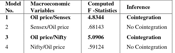
decided by Akaike Information Criterion (AIC). Results of table 3 shows that when

oil price (oil price/Sensex and oil price/nifty) is the dependent variable, the

calculated F-statistics is found to be higher at 99% of level of significance than the

upper critical bound values of peasarn et al (1996). This supports the assertion that

there exists a long- run cointegration relation between oil prices with sensex and

nifty when the oil price is the dependent variables.

As evidence from table 3, reverse cointegration relationship is not found when the

sensex and nifty are the dependent variables as the F- statistics are lower at 95% upper

critical bounds values.

Table 3 F- Statistics of Co-integration

Model No.

Macroeconomic Variables

Computed

F -Statistics Inference

1 Oil price/Sensex 4.8344 Cointegration

2 Sensex/Oil price .68143 No Cointegration

3 Oil price/Nifty 5.0906 Cointegration

4 Nifty/Oil price .59124 No Cointegration

Note: Pesaran et al. 2001, the critical values are estimated with the assumption of unrestricted intercept term with no trend. * Indicates the level of significance at 10%, (2.72 -2.72) ** indicates the level of significance at 5 % (3.23-4.35) and *** indicates the level of significance at 1 %. (4.29 - 5.61) (Pesaran tabulated lower and upper band values are given parentheses).

Based on the existence of cointegration relationship for model one and model three, the

following long run coefficients are estimated (Table 4). The resulting underlying ARDL

equation was also verified with all its statistical diagnostic properties in order to get

Table 4 Estimated Long Run Coefficients using the ARDL (3)*: Sensex and Nifty

*ARDL (3) selected based on Akaike Information Criterion

From Table 4, which brings out the precise nature of the long run relationship when oil

price is the dependent variable, the following inferences can be drawn: the long run

coefficient of sensex and nifty is found to be positive and significant supporting the

long run effect on oil prices. It means changes in the stock prices have impact on oil

prices.

Table 5 Error Correction Representation for the Selected ARDL (3)*: Sensex Model

Regressor Coefficient

Standard

Error T-Ratio [Prob]

dOILPRICE1 .370 .081 4.55 [.000] dOILPRICE2 .211 .084 2.50 [.014]

dC 2.24 .935 2.40 [.018]

dSENSEX .7618E-3 .1423E-3 5.35 [.000] ecm(-1) -0.17 .030 -5.75 [.010] *ARDL (3) selected based on Akaike Information Criterion

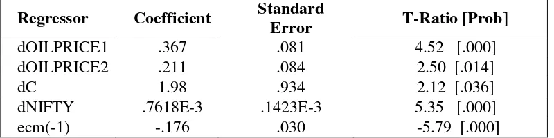
Table 5. Error Correction Representation for the Selected ARDL (3)*: Sensex Model

Regressor Coefficient Standard

Error T-Ratio [Prob]

dOILPRICE1 .367 .081 4.52 [.000] dOILPRICE2 .211 .084 2.50 [.014]

dC 1.98 .934 2.12 [.036]

dNIFTY .7618E-3 .1423E-3 5.35 [.000] ecm(-1) -.176 .030 -5.79 [.000]

Regressor

Coefficient

Standard Error

T-Ratio [Prob]

Sensex Model

C 12.83 4.75 2.69 [.008] Sensex .004 .4149E-3 10.49 [.000] Nifty Model

Table 5 and 6 provides the Error Correction Representation for the Sensex and Nifty

model. The error correction term ecm(-1), which measures the speed of adjustment to

restore equilibrium in the dynamic model, appear with negative sign and is statistically

significant at 1 percent level ensuring that long run equilibrium can be attained. The

coefficient of ecm(-1) for both models, is equal to -0.176 for short run model implying

that the deviation from the long-term inequality is corrected by 17.6 % percent over

each year.

Conclusion

The findings of this study conclude that despite the India‟s aggressive economic

growth in the past fifteen years, the volatility of stock prices in India have a significant

impact on the volatility of oil prices.While dynamics in the oil prices not impacted the

price creation process of equities in Indian stock markets. India is quite unique in a

sense that they are less affected by the recent Global financial crisis. Also, there are

macroeconomic factors that have had a strong impact over equity returns and volatility

in these equity markets. These factors appear to have had a much greater role in

Appendix 1

Table A1 Diagnostic Tests Nifty model

Item Test Applied CHSQ(2) Prob

Serial correlation Lagrange multiplier test 20.52 .058 Normality test of skewness and kurtosis 1.04 .307 Functional Form Ramsey's RESET test 3.10 .051 Heteroscedasticity White test 21 .59 .049

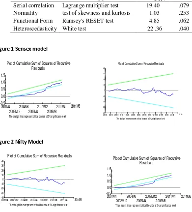
Table A2 Diagnostic Tests sensex model

Item Test Applied CHSQ(2) Prob

Serial correlation Lagrange multiplier test 19.40 .079 Normality test of skewness and kurtosis 1.03 .253 Functional Form Ramsey's RESET test 4.85 .062 Heteroscedasticity White test 22 .36 .040

Figure 1 Sensex model

Plot of Cumulative Sum of Squares of Recursive Residuals

The straight lines represent critical bounds at 5% significance level

-0.5 0.0 0.5 1.0 1.5

2001M4 2004M8 2007M12 2011M4 2002M12 2006M4 2009M8

2011M6

Plot of Cumulative Sum of Recursive Residuals

The straight lines represent critical bounds at 5% significance level

-10 -20 -30 -40 0 10 20 30 40

2001M42002M2 2002M12 2003M10 2004M82005M62006M42007M2 2007M12 2008M10 2009M8 2010M62011M4 2011M6

Figure 2 Nifty Model

Plot of Cumulative Sum of Recursive Residuals

The straight lines represent critical bounds at 5% significance level -10 -20 -30 -40 0 10 20 30 40

2001M4 2002M12 2004M8 2006M4 2007M12 2009M8 2011M4 2011M6

Plot of Cumulative Sum of Squares of Recursive Residuals

The straight lines represent critical bounds at 5% significance level

-0.5 0.0 0.5 1.0 1.5

2001M4 2004M8 2007M12 2011M4 2002M12 2006M4 2009M8

2011M6

References:

Anoruo, E., & Mustafa, M., (2007) “An empirical investigation into the relation of oil to stock market prices”, North American Journal of Finance and Banking Research, 1(1), pp. 22-36.

Bashar, Z. (2006), “Wild oil prices, but brave stock markets! The case of Gulf Cooperation Council (GCC) stock markets”, Middle East Economic Association Conference, Dubai.

Bhar, Ramaprasad and Nikolova, Biljana (2009) “Oil Prices and Equity Returns in the

BRIC Countries” “The World Economy” doi: 10.1111/j.1467-9701.2009.01194.x

Ciner C. (2001), “Energy Shocks and Financial Markets: Nonlinear Linkages”, Studies in

Non- Linear Dynamics and Econometrics, 5, 203-212.

Chen, N.-F., Roll, R., and S.A. Ross (1986), “Economic Forces and the Stock Market,”

Journal of Business, 59, 383-403.

Chittedi, Krishna Reddy (2010) “Global Stock Markets Development and Integration: with Special Reference to BRIC Countries” ‘International Review of Applied Financial

issues and Economics‟, Vol 2, Issue 1, March.

Chittedi, Krishna Reddy (2011) “Integration of International Stock Markets: With Special Reference to India” „GITAM Journal of Management, Vol 9, No 3.

Cologni, A. and Manera M. (2008), “Oil prices, inflation and interest rates in a

structural cointegrated VAR model for the G-7 countries.” Energy Economics, 30, 856-88.

Hamilton, J. D. (2003), “What is an Oil Shock?” Journal of Econometrics, 113, pp. 363-98.

Hammoudeh, S., and E., Aleisa (2004). Dynamic relationship among GCC stock markets and NYMEX oil futures. Contemporary Economic Policy, Vol. 22, pp. 250–69.

Huang, R.D., Masulis, R.W., Stoll, H.R., (1996) “Energy shocks and financial markets”.

Journal of Futures Markets 16, 1–27.

Jones, C., Kaul, G., (1996) “Oil and the Stock Market”, Journal of Finance, 51, pp 463-491.

Kilian, L., (2008), “Exogenous Oil Supply Shocks: How Big Are They and How Much

Do They Matter for the US Economy?” Review of Economics and Statistics, 90, 216-40.

Kwiatkowski, D., Phillips, P. C. B., Schmidt, P., Shin, Y., (1992) “Testing the null

hypothesis of stationarity against the alternative of a unit root.” Journal of Econometrics

Maghyereh, A.,(2004).“Oil price shock and emerging stock markets: A Generalized VAR Approach”, International Journal of Applied Econometrics and Quantitative Studies, 1(2), pp. 27-40.

Miller, J.I. and Ratti, R.A. (2009). “Crude oil and stock markets: Stability, instability,

and bubbles.” Energy Economics, 31, 559-568.

Narayan, K., P.,and Narayan, S., (2010). “Modeling the impact of oil prices on

Vietnam‟s stockprices”, Applied Energy, 87, pp. 356-361.

O'Neil, T.J., Penm, J., Terrell, R.D.,( 2008) “The role of higher oil prices: A case of major

developed countries”. Research in Finance 24, 287–299.

Papapetrou, E., (2001) “Oil price Shocks, Stock Market, Economic Activity and

Employment In Greece.”Energy Economics 23, 511-532.

Pesaran, M. H., Shin, Y. and Smith, R. J. (2001), “Bounds Testing Approaches to the

Analysis of Level Relationships”, Journal of Applied Econometrics, 16: 289–326.

Ravichandran K (2010) “Impact of Oil Prices on GCC Stock Market” Research in Applied

Economics, 2010, Vol. 2, No. 1.

Zhang D. (2008),”Oil shock and economic growth in Japan: A nonlinear approach”,