Detecting big structural breaks in large factor models

Munich Personal RePEc Archive

Detecting big structural breaks in large

factor models

Chen, Liang and Dolado, Juan Jose and Gonzalo, Jesus

Universidad Carlos III de Madrid

8 June 2011

Online at

https://mpra.ub.uni-muenchen.de/31344/

Detecting Big Structural Breaks in Large Factor

Models

∗

Liang Chen

Juan J. Dolado

Jesús Gonzalo

This Draft: June 2, 2011

Abstract

Constant factor loadings is a standard assumption in the analysis of large dimen-sional factor models. Yet, this assumption may be restrictive unless parameter shifts are mild. In this paper we develop a new testing procedure to detectbig breaks in factor loadings at either known or unknown dates. It is based upon testing for struc-tural breaks in a regression of the first of the ¯r factors estimated by PC for the whole sample on the remaining ¯r₋1 factors, where ¯ris chosen using Bai and Ng´s (2002) information criteria. We argue that this test is more powerful than other tests available in the literature on this issue.

KEYWORDS: Structural break,large factor model, factor loadings, principal compo-nents.

JELCODES: C12, C33.

∗_{We are grateful to Soren Johansen, Hashem Pesaran and participants at the Conference in Honour of}

Sir David F. Hendry (St. Andrews) and the Workshop on High-Dimensional Econometric Modelling (Cass Business School). Financial support from the Spanish Ministerio de Ciencia e Innovación (grants SEJ2007-63098 and Consolider-2010) and Comunidad de Madrid (grant Excelecon) is gratefully acknowledged.

1

Introduction

Despite the well-ackowledged fact that some parameters in economic relationships can become unstable due to important structural breaks (e.g., those related to technological change, globalization or strong policy reforms), a standard practice in the estimation of large factor models is to assume the constancy of the factor loadings. Possibly, one of the main reasons for this benign neglect of breaks is that the first attempt to address this issue, by means of time-varying factor loadings, focused on characterizing the properties of mild instabilities, under which the constructed factors using principal components (PC hereafter) remain consistently estimated (Stock and Watson, 2002).

Later on, however, a few studies have investigated the performance of factor-based forecasting subject not only to mild but also to large breaks in the factor model structures. Banerjee, Marcellino and Masten (2008) conclude that the instability of factor loadings is the most likely reason behind the worsening factor-based forecasts, particularly in small samples. Although their results are exclusively based on Monte Carlo simulations, they shed some light on the importance of detecting relevant structural breaks in the factor loadings. Two additional papers have contributed to this stream of research. The first one is by Stock and Watson (2009) who, extending their previous approach, propose several forms of mild structural instability in factor models to then use empirical evidence showing that the failure of factor-based forecasts is mainly due to the instability of forecast function, rather than of the factor loadings. As a result, they conclude that the estimated factors using PC are still consistent when instabilities are small in magnitude and independent, claiming therefore that forecasts can be improved by using full sample factor estimates and subsample forecasting equations. Yet, this focus on mild structural breaks, though very useful, has also been questioned by Giannone (2007) who argues that"....to understand structural changes we should devote more effort in modelling the variables characterized by more severe instabilities...". In this paper, we follow this route by proving a precise characterization of the different conditions under which big and mild structural breaks in the factor loadings may occur, as well as develop a test to distinguish between them. We conclude that the influence of big breaks cannot be ignored since it may lead to misleading results in the usual econometric practices with factor models.

claimed that the number of factors can be correctly estimated using subsamples before and after the known break date. However, if either the break date is not considered to be a priori known or the number of factors is not correctly specified, their test may exhibit poor power. For example, as explained below, a factor model withrcommon factors and 1 structural break in the factor loadings admits a standard factor representation withr+1 common factors without a break. Hence, if the number of factors is incorrectly specified as beingr+1 instead ofr, their test may not detect any break at all.1

Our contribution in this paper is to propose a simple testing procedure to detect struc-tural breaks in the factor loadings which allows for different types of breaks and does not suffer from the previous shortcomings. In particular, we first derive some asymptotic re-sults finding that, in contrast to small breaks where both the number of factors and the factor space are consistently estimated, the number of factors will be over-estimated when big breaks occur. We argue that ignoring those big breaks can have serious consequences on the forecasting performance of factors in some popular regression models. We then propose a simple two-step test procedure for testing big breaks. In the first step, the num-ber of factors for the whole sample period is estimated as ˆr, and then the ˆr factors are estimated using PC. In the second step, one of the estimated factors (e.g., the first one) is regressed on the remaining ˆr₋1 factors, and the standard Chow Test or the Sup Type Test of Andrews (1993), depending on whether the date of the break is treated as known or unknown, is then used to test for a structural break in this regression. If the null of no structural breaks is rejected in the second-step regression, we conclude that there are big breaks and, otherwise, that either no breaks at all exist or that only small breaks occur. We also illustrate the finite sample performance of our test using simulations, as well as provide an empirical application of how to implement our testing approach.

The rest of the paper is organized as follows. In Section 2, we present the basic no-tation, assumptions and give precise definitions of two different types of structural breaks considered here: bigandsmall breaks. In Section 3, we analyze the consequences of big breaks on the choice of the number of factors and their estimation, as well as the effects of those breaks on the factor augmented regressions. In Section 4, we derive the asymptotic results underlying our approach and discuss the advantages of our proposed test against Breitung and Eickmeier’s (2010) test. Section 5 deals with the finite sample performance of our test procedure using Monte-Carlo simulations. Section 6 provides two empirical applications. Finally, Section 7 concludes.

2

Notation and Preliminaries

We consider factor models that can be rewritten in the static canonical form:

Xt=AFt+et (1)

1_{Even when the break date is known, the number of factors could still be incorrectly estimated due to}

whereXt is the N×1 vector of observed variables,A= (α1, . . .,αN)′is theN×rmatrix of factor loadings,ris the number of common factors,Ft = (ft1, . . . ,ftr)′is ther×1 vec-tor of common facvec-tors, andet is the N×1 vector of idiosyncratic errors. In the case of dynamic factor models, all the common factors ft and their lags are stacked intoFt. Thus, a dynamic factor model withr dynamic factors and plags of these factors can be written as a canonical static factor model with(r+1)_×p static factors. Further, given the as-sumptions we make about theet error terms, the case analyzed by Breitung and Eickmeier (2010) where theeit disturbances are generated by individual specific AR(pi) processes is also considered. Notice, however, that our setup excludes the generalized dynamic factor models considered by Forni and Lippi (2001) when the polynomial distributed lag tends possibly to infinity.

We assume that there is a single structural break in the factor loadings of all factors at the same timeτ:

Xt=AFt+et t=1,2. . . ,τ (2)

Xt=BFt+et t=τ+1, . . . ,T (3)

whereB= (β1, . . .,βN)′is the new factor loadings after the break. By defining the matrix

C=B₋A, which captures the size of the breaks, the factor model in (2) and (3) can be rewritten as:

Xt=AFt+CGt+et (4)

whereGt=0 fort=1, . . .,τ, andGt =Ft fort=τ+1, . . .,T.

As argued by Stock and Watson (2002), the effects of some mild instability in the factor loadings can be averaged out, so that estimation and inference based on PC remain valid. Our aim is to generalize their analysis by distinguishing between two types of break sizes:bigandsmall. Whereas the latter correspond to those breaks characterized by Stock and Watson (2002, 2009) and therefore can be neglected, our goal is to analyze which are the effects of the former.We we will show that they cannot be ignored. Thus, to distinguish between both types of breaks, it is convenient to partition the matrixCas follows:

C= [Λ H]

whereΛandH areN_×k1 andN×k2 matrices that corresponds to thebigand thesmall

breaks, andk1+k2=r. In other words, we assume that, among the r factors,k1 and k2

factors are subject tobigandsmallbreaks in their loadings, respectively. Accordingly, we can also partitionGt into two parts,Gt1andGt2, such that (4) can be rewritten as:

Xt =AFt+ΛGt1+HG2t +et (5)

whereΛ= (λ1, . . . ,λN)′andH= (η1, . . .,ηN)′.

Once the basic notation has been established, the next step is to provide precise defini-tions of the two types of breaks.

a. E_||λi||4<∞. N−1∑Ni=1λiλi′→ΣΛas N →∞for some positive definite matrixΣΛ.

b. ηi=Op(√_NT1 )for i=1,2, . . .,N.

The matricesΛandHare assumed to contain random elements. Assumption 1.a yields the definition of a big break which also includes the case whereλi=0 ( no break) for a fixed proportion of variables as N _→∞. Assumption 1.b, in turn, provides the definition of small breaks which can be ignored asN andT goes to infinity.

To investigate the influence of the breaks on the estimation of factors and the number of factors, some further assumptions need to be imposed. To achieve consistent notation with the previous literature in the discussion of these assumptions, we follow the presentation of Bai and Ng (2002) with a few slight modifications. Lettr(Σ)and_||Σ_||=ptr(Σ′Σ_)denote

the trace and the norm of a matrixΣ, respectively, while[Tπ]denotes the integer part of

T_×π forπ_∈(0,1). Then

Assumption 2.Factors: E(Ft) =0, E||Ft||4<∞, T−1∑Tt=1FtFt′→ΣF and T−1∑τt=1FtFt′→ π∗_{ΣF as T →∞for some positive definite matrixΣF whereπ}∗_=lim

t→∞Tτ.

Assumption 3. Factor Loadings: E_||αi||4≤M<∞, and N−1A′A→ΣA, N−1Γ′Γ→ΣΓ

as N_→∞for some positive definite matrixΣAandΣ_Γ, whereΓ= [A Λ].

Assumption 4. Idiosyncratic Errors: the error terms et, the factors Ft and the loadings

Aisatisfy the Assumption A, B, C, E, F1 and F2 of Bai (2003).

Assumption 5. Independence of Factors, Loadings, Breaks, and Idiosyncratic Errors:

[Ft]T_t=1,[αi]N_i=1,[λi]N_i=1,[ηi]N_i=1and[et]T_t=1are mutually independent groups, and for all i

1

√

T

T

∑

t=1

Fteit =Op(1).

3

The Effects of Structural Breaks

In this section, we study the effects of the structural breaks on the estimation of factors based on PC, and on the estimation of the number of factors based on the information criteria proposed by Bai and Ng (2002). Our main result is that the estimated factors using PC are not consistent and the number of factors tends to be overestimated when big breaks exist, in contrast to Stock and Watson’s (2002, 2009) findings that the true factor space is still consistently estimated.

3.1

The estimation of factors

Let us rewrite model (5) withk1big breaks andk2small breaks in the more compact form:

Xt =AFt+ΛGt1+εt (6)

whereεt=HGt2+et. The idea is to show that the new error terms εt still satisfy the nec-essary conditions for (6) being a standard factor model with new factorsF_t∗= [F_t′ G_t1′]′

and new factor loadings[A Λ].

Let ¯r be the selected number of factors, either by the information criteria or by some prior knowledge. Note that ¯r is not necessarily equal to r. Let ˜F be √T times the ¯r

eigenvectors corresponding to the ¯rlargest eigenvalues of the matrixX X′, and define

ˆ

F =_FV˜ _N,T

as the estimated factors, where theT_×NmatrixX= [X1¯ ,X2¯ . . .X¯T]′, ¯Xt= [Xt1,Xt2, . . . ,XtN]′, ˆ

F= [_Fˆ_1,Fˆ_{2, . . . ,F}ˆ_T]′_{, andV}

N,T is a diagonal matrix with the ¯rlargest eigenvalues of(NT)−1X X′. Then we have

Proposition 1. For any fixed r¯_≥1, under Assumptions 1 to 5, there exists a full rank

¯

r_×(r+k1)matrix D andδN,T =min{

√

N,√T_}such that:

ˆ

Ft=DFt∗+Op(1/δN,T) (7)

This result implies that ˆFt estimate consistently the space of the new factors, Ft∗, but not the space of the true factors,Ft.

Let us consider two cases. First, whenk1=0 ( no big breaks), we have that Gt1=0, andF_t∗=Ft, so that (7) becomes

ˆ

Ft=DFt+Op(1/δN,T) (8)

for a ¯r_×rmatrixDof full rank. This just trivially replicates the well-known consistency result of Bai and Ng (2002).

Secondly, in the more interesting case whenk1>0 (big breaks exist), we can rewrite

(7) as

ˆ

Ft= [D1 D2]

Ft

G_t1

where the ¯r_×(r+k1) matrix D is partitioned into the ¯r×r matrix D1 and the ¯r×k1

matrixD2. Note that, by the definition ofGt, G1t =0 fort=1,2, . . .,τ, andG1t =Ft1for

t=τ+1, . . . ,T, whereF_t1is thek1_×1 sub-vector ofFt that experiences big breaks in their loadings. Therefore (9) can be expressed as:

ˆ

Ft=D1Ft+op(1)fort=1,2, . . .,τ (10) ˆ

Ft=D∗2Ft+op(1)fort=τ+1, . . .,T (11)

whereD∗₂=D1+[D2 0], 0 is a ¯r×(r−k1)zero matrix, such thatD26=0 sinceDis a

full-rank matrix. Hence, sinceD1₆=D∗₂, this result implies that, in contrast to small breaks, the estimated factors ˆF are not consistent for the space of the true factorsF under big breaks. Thus, in this case, the use of estimated factors as predictors or explanatory variables may lead to misleading results in the usual econometric practices with factor models.

To illustrate the consequences of having big breaks in the factor loadings, consider the following simple Factor Augmented Regression (FAR) model (see Bai and Ng, 2006):

yt =a′Ft+b′Wt+ut, t=1,2, ..,T (12)

whereWt is a small set of observable variables and ther×1 vector Ft contains the r common factors driving a large panel datasetxit (i=1,2, ...N;t=1,2, ...T) which excludes bothytandWt.The parameters of interest are the elements of vectorbwhileFt is included in (12) to control for potential endogeneity arising from omitted variables. Since we cannot identifyFt anda, only the producta′Ft is relevant. Suppose there is a big break at dateτ. From (10) and (11), we can rewrite (12) as:

yt= (a′D−₁)(D1Ft) +b′Wt+ut fort=1,2, . . .,τ

yt = (a′D∗−₂ )(D∗2Ft) +b′Wt+ut fort=τ+1, . . . ,T

whereD−₁D1=D∗−₂ D2=Ir, or equivalently

yt=a′1Fˆt+b′Wt+u˜t fort =1,2, . . .,τ (13)

yt=a′2Fˆt+b′Wt+u˜t fort =τ+1, . . . ,T (14)

wherea′₁=a′D−₁ anda′₂=a′D∗−₂ , and ˜ut =ut+op(1).

If the number of factors is assumed to be known a priori , ¯r =r, then D−₁ =D−₁1,

D∗−₂ =D∗−₂ 1. SinceD16=D∗₂, it follows that D−₁16=D₂∗−1 and thusa16=a2. Therefore,

using the indicator function_I(t >τ), (13) and (14) can be rewritten as

are many examples in the literature where the number of factors is a priori imposed for theoretical reasons, e.g., to name a few, a single common factor representing a global effect is assumed in the well-known study by Bernanke, Boivin and Eliasz (2005) on measuring the effects of monetary policy in Factor Augmented VAR (FAVAR) models, or two factors are imposed by Rudebusch and Wu (2008) in their macro-finance model.

Alternatively, if the number of factors is not assumed to be apriori known and therefore needs to be estimated using some information criteria, we will show in Proposition 2 in the next section that the chosen number of factors will tend tor+k1 as the sample size

gets large. In this case,D1 andD2 are(r+k1)×r, and by the definitions ofD1 andD∗2,

it is easy to show that we can always find ar_×(r+k1)matrixD∗=D−1 =D∗−2 such that D∗D1=D∗D∗₂=Ir. If we define

a∗=a′D∗ (16)

thena′₁=a′₂=a∗so that (13) and (14) can be rewritten as

yt=a∗Fˆt+b′Wt+u˜t, t=1,2, ..,T (17)

From above equation we can see that the estimation of (12) will not be affected by the estimated factors under big breaks if ¯r=r+k1.

In sum, in the presence of big breaks, the use of estimated factors as the true factors when assuming that the number of factors is a priori known will lead to inconsistent es-timates in a FAR. As a simple remedy, ˆFtI(t >τ) should be added as regressors when big breaks are detected and the break date is located. Alternatively, without pretending to know a priori the true number of factors, the estimation of FAR will be robust to the estimation of factors under big breaks if the number of factors is overestimated. Notice that a similar argument will render inconsistent the impulse response functions in FAVAR models where (12) becomesyt+1= (Ft+1,Wt+1)´. As a result, in order to run regression

(17), a formal test of whether big breaks exist is required.We will illustrate these points by using simulations in a typical forecasting exercise where the predictors are common factors estimated by PC.

3.2

The estimated number of factors

Breitung and Eickmeier (2010) have previouosly argued that the presence of structural breaks in the factor loadings may lead to the overestimation of the number of factors but they do not prove this result. In this part, we fill this gap by providing a rigorous proof.

Let ˆr be the estimated number of factors in (6) using the information criteria of Bai and Ng (2002). Then the following result holds:

Proposition 2. Under Assumptions 1 to 5, it holds that

lim

When there is no big break (k1=0), this result replicates Theorem 2 of Bai and Ng

(2002). However, under big breaks (k1>0), their information criteria will overestimate

the number of factors by the number of big breaks (k1). Actually, Bai and Ng (2002)’s criteria, that consistently estimate the number of true factors, will overestimate the number of original factors when there are big breaks because we have shown that a factor model with those breaks admits a representation without break but with more factors.

Finally, notice that, although the presence of structural breaks in the factor loadings may lead to wrong estimation of the factor space and the number of factors, the common part of a factor model (AFt andBFt) can still be consistently estimated if enough factors are extracted.

4

Testing for Structural Breaks

4.1

Hypotheses of interest and test statistics

From the previous discussion, we have found that the factor space and the number of factors are both consistently estimated only when mildl breaks exist. Therefore, our goal here is to develop a test for big breaks.

If we were to follow the usual approach in the literature to test of structural breaks, we should consider

H0:A=B H1:A6=B

However, if only small breaks occur, the alternative hypothesis may not be interesting sinceC=A₋Bvanishes asN _→∞andT _→∞. Thus, this kind of local alternatives for which the usual test should have no trivial power, is not relevant for the large factor models we consider here. Therefore, since our focus is on big breaks, we consider instead:

H0:k1=0

H1:k1>0

where the null and alternative hypotheses correspond to the cases where there are no big breaks (yet there may be small breaks) and there is at least one big break, respectively.

To test the above null hypothesis, we consider the following two-step procedure:

1. In the first step, the number of factors to estimate,r , is either determined by Bai and¯

Ng ´s (2002) information criteria (r¯=r) or by prior knowledge, so thatˆ r common¯

factors (Fˆt) are estimated by PC.

2. In the second step, we consider the following linear regression of the first estimated factor on the remainingr¯₋1ones:

ˆ

whereFˆ₋1t= [Fˆ2t···Fˆrt¯]′and c= [c2···cr¯]′are(r¯−1)×1vectors. Then we test for a structural break of c in the above regression. If a structural break is detected, then we reject H0:k1=0; otherwise, we cannot reject the null stating that there are no big breaks.

Both steps can be easily implemented in practice. In the second step, although there are many methods of testing for structural breaks in a simple linear regression model, we consider the Chow Test when the possible break date is assumed to be known, and the

Sup-type Test when no prior knowledge about the break date exists. Moreover, since the Wald, LR, and LM test statistics have the same asymptotic distribution under the null, we focus on the LM and Wald tests because they are simpler to compute.

Following Andrews (1993), the LM test statistic is defined as:

L₍π_{¯) =} T

¯

π(1₋π¯)

1

T

τ

∑

t=1

ˆ

F₋1tuˆt ′

ˆ

S−11 T

τ

∑

t=1

ˆ

F₋1tuˆt

(19)

where ¯π=τ/T, ˆutis the residuals in the OLS regression of (18),S=limT→∞Var

1 √

T ∑ T

t=1Fˆ−1tut

,

and ˆSis a consistent estimate ofS. The Sup-LM statistic is defined as:

L₍Π_{) =sup}

π∈Π T

π(1₋π)

1

T

[Tπ]

∑

t=1

ˆ

F₋1tuˆt ′

ˆ

S−1

1

T

[Tπ]

∑

t=1

ˆ

F₋1tuˆt

(20)

whereΠis some pre-specified subset of[0,1].

Similarly, the Wald and Sup-Wald test statistics can be constructed as:

L∗₍π_{¯) =Tcˆ1(}π_¯)−cˆ2(π_¯)′_Vˆ−1_cˆ1(π_¯)−cˆ2(π_{¯) (21)}

and

L∗₍Π_{) = sup}

π∈Π

Tcˆ1(π)−cˆ2(π)

′ ˆ

V−1cˆ1(π)−cˆ2(π)

(22)

where ˆc1(π)and ˆc2(π)are OLS estimates ofcusing subsamples before and after the break

point : [Tπ]. In addition, ˆV =_Mˆ−1_SˆMˆ−1_{, and ˆM=T}−1_∑T

t=1Fˆ−1tFˆ₋′1t.

To illustrate why our two-step procedure is able to detect the big breaks, it is useful to consider a simple example wherer=1,k1=1 (one common factor and one big break). Then (6) becomes:

Xt=A ft+Λgt+εt

wheregt =0 fort=1, . . .,τ, andgt = ft fort =τ+1, . . . ,T. By Proposition 2, we will tend to get ˆr=2 in this case. Suppose now that we estimate 2 factors (¯r=2). Then, by Proposition 1, we have:

_ˆ

ft1

ˆ

ft2

=D

ft

gt

whereD=

d1 d2 d3 d4

is a non-singular matrix. By the definition ofgt we have:

ˆ

ft1=d1ft+op(1) fˆt2=d3ft+op(1) for t=1, . . .,τ

ˆ

ft1= (d1+d2)ft+op(1) fˆt2= (d3+d4)ft+op(1) for t=τ+1, . . . ,T

which imply that:

ˆ

ft1= d1 d3

ˆ

ft2+op(1) for t=1, . . .,τ

ˆ

ft1=

d1+d2 d3+d4

ˆ

ft2+op(1) for t =τ+1, . . .,T

Thus, we can observe that the two estimated factors are linearly related and that the co-efficients d1

d3 and

d1+d2

d3+d4 before and after the break date must be different due to the

non-singularity of the matrixD. As a result, if we regress one of the estimated factors on the other and test for a structural break in this regression, we should reject the null of no big break. We choose the first estimated factor, ˆft1,as the regressand in the previous

regres-sions because being the "main factor" in the PC analysis it is likely thatd36=0.2Likewise,

if the break dateτis not a priori assumed to be known, the Sup-type Test will yield a natu-ral estimate ofτ at the date when the test reaches its maximum value. In what follows, we derive the asymptotic distribution of the test statistics (19) and (20) under the null hypoth-esis, as well as extend the intuition behind this simple example to the more general case in order to show that our test has power against relevant alternatives.

4.2

Limiting distributions under the null hypothesis

Since in most applications, the number of factors is estimated by means of the information criteria, and it converges to the true one under the null hypothesis of no big break, we start with the most interesting case where ¯r=r.

Note that use of PC implies that ∑_tT₌₁Fˆ₋1tFˆ1t =0 for anyT by construction, so we have ˆc=0 in (18) and ˆut =Fˆ1t in (19). To derive the asymptotic distributions of the LM statistics, we impose the following additional assumptions:

Assumption 6. √T/N_→0as N _→∞and T _→∞. .

Assumption 7. _{Ft}is a stationary and ergodic sequence, and{FitFjt−E(FitFjt),Ωt}is

an adapted mixingale withγmof size−1for i,j=1,2, . . .,r, that is:

r

E

E(Yi j,t|Ωt−m)2

≤ctγm

where Yi j,t =FitFjt−E(FitFjt),Ωt is a σ−algebra generated by the information at time

t,t₋1, . . .,_{ct}and{γm}are non-negative sequences andγm=O(m−1−δ)for someδ >0.

2_{SinceDis non singular, even ifd}

3=0,d1cannot be equal to zero. If the regression for the first

sub-sample yields an ill-defined (ie., very large) estimated slope, then we recommed using ˆft2as the regressand

Assumption 8. For the subsetΠof[0,1]:

sup π∈Π

1

√

NT

Tπ

∑

t=1

N

∑

i=1

αiFt′eit

2

=Op(1)

Assumption 9. Sˆ−S

=o_p(1), and S is a(r−1)×(r−1) symmetric positive definite

matrix.

Assumption 6 and 8 are required to bound the estimation errors of ˆFt, while Assump-tion 7 is necessary for deriving the weak convergence of the test statistics using the Func-tional Central Limit Theorem (FCLT).

Note that these assumptions are not restrictive. Assumption 6 allowsT to beO(N1+δ)

for₋1<δ <1. As for Assumption 7, it allows one to consider a quite general class of linear processes for the factors: Fit =∑∞k=1φikvi,t−k, wherevt = [v1t. . .vrt]′ are i.i.d with zero means, andVar(vit) =σ_i2<∞. It can shown that in this case:

r

E

E(Yi j,t|Ωt−m)2

≤σiσj ∞

∑

k=m

|φik| ! _∞

∑

k=m

|φjk| !

then it suffices that

∞

∑

k=m

|φik| !

=O(m−1/2−δ)

for someδ >0, which is satisfied for a large class of ARMA processes. Assumption 8 is analogue to Assumption F.2 of Bai (2003), which involves zero- mean random variables. Finally, a consistent estimate ofScan be calculated by a HAC estimator.

Let ”_→d ”denote convergence in distribution , and W_{r−1(·) denote a r−1 vector of}

standard Brownian Motions, then:

Theorem 1. Under the null hypothesis H0:k1=0and Assumptions 1 to 9:

L₍Π_)→d _sup

π∈Π

W_r−1(π₎₋πW_r−1(1)′W_r−1(π₎₋πW_r−1(1)/[π₍₁₋π_)];

L₍π_¯)→d χ2_(r−1).

The critical values for the Sup-type test are provided in Andrews (1993).

4.3

Behavior of LM and Wald tests under the alternative hypothesis

We extend the idea of the simple example in section 4.1 to show that, under the alternative hypothesis (k1>0), the linear relationship between the estimated factors changes at time

τ, so that big breaks can be detected.

First, let us consider the case wherer<r¯_≤r+k1 so thatD1andD∗₂in (10) and (11) become ¯r_×rmatrices with full column rank. Notice that, sincer<r¯, we can always find ¯

r_×1 vectorsρ1 andρ2 which belong to the null spaces ofD′1andD∗ ′

2 separately, that is,

ρ′

1D1=0 andρ2′D2∗=0. Hence, premultiplying both sides of (10) and (11) byρ1′ andρ2′

leads to:

ρ′

1Fˆt=op(1) t=1,2. . .,τ ρ′

2Fˆt=op(1) t=τ+1, . . .,T,

which, after normalizing the first elements ofρ1andρ2to be 1, yields:

ˆ

F1t=Fˆ′−1tρ1∗+op(1) t=1,2. . .,τ (23) ˆ

F1t=Fˆ′−1tρ2∗+op(1) t=τ+1, . . . ,T (24)

Next, to show that ρ₁∗ ₆= ρ₂∗, we proceed as follows. Suppose that γ _∈ Null(D′₁) and γ ∈Null(D∗₂′), then by the definition of D1 and D∗₂ and by the basic properties of

full-rank matrices, it holds that γ _∈Null(D′). Since Dis full rank ¯r_×(r+k1) matrix, then

Null(D′) =0 and thusγ =0. Therefore, the only vector that belongs to the null space of

D1andD∗₂ is the trivial zero vector. Further, because the rank of the null space ofD1and D∗₂is ¯r₋r>0, we can always find two non- zero-vectors such thatρ16=ρ2.

Notice that when ¯r_≤r, the rank of the null spaces ofD1andD∗₂becomes zero. Hence,

the preceding analysis does not apply in this case despite the existence of linear relation-ships among the estimated factors. If we regress one of the estimated factors on the others, with ˆρ1and ˆρ2denoting the OLS estimates of the coefficients using the subsamples before

and after the break, it is easy to show that ˆρ1→θ1 and ˆρ2→θ2, but generally we cannot

verify thatθ16=θ2.

In the case where ¯r>r+k1, the rank of null space of D defined in Proposition 1

becomes ¯r₋(r+k1). Applying similar arguments as above, we can find a non zero ¯r_×1 vectorρ such thatρ′D=0. Then, premultiplying both sides of (7) byρ′and normalizing the first element ofρ to be 1, it follows that:

ˆ

F1t=Fˆ′−1tρ∗+op(1)fort=1,2, . . .,T

Hence, there is still a linear relationship between the estimated factors, but this relationship (ρ∗) is constant over time.

As a result, our test may fail to detect the breaks when ¯r_≤r or ¯r>r+k1, which is

estimated ones, ( ¯r=rˆ)and we have shown that_P[rˆ=r+k1]→1. Secondly, instead of

using a single value, we can try different values of ¯r.Then, under the null, we should not detect any break no matter which value of ¯rwe use while, under the alternative, we should detect breaks when ¯rlies betweenrandr+k1.

4.4

Comparison with other available tests

Although the issue of instability in factor models was initially raised by Stock and Watson (2002) in the context of small breaks, Breitung and Eickmeier (2010) (BE test, henceforth) is, to our knowledge, the only available paper that proposes a test for big breaks. Thus, it is natural to compare our testing procedure with theirs. In our view, the BE test suffers from three shortcomings which are worth mentioning before the comparison is made.

First, the BE test will lose power when the number of factors is overestimated. The BE test is equivalent to the Chow test in the regressionXit =αiFt+eit whereFt is replaced by

ˆ

Ft. However, as shown in equation (5), a factor model with big breaks in the factor loadings admits a new representation with more factors but no break. In other words, when the number of factors is overestimated, the PC estimators consistently estimate (up to a linear transformation) the new factors and loadings which are stable in the new representation. Thus the BE test may fail to detect breaks in this case. Although the authors are fully aware of this problem (see Remark B in their paper) and suggest to split the sample to estimate the correct number of factors, in principle this is not feasible when the break date is considered to be unknown. Using a Sup-Type Test, as BE propose, solves the problem of the unknown break date but, since the number of factors will tend to be overestimated, lack of power will still be a problem.

Secondly, their testing procedure is mainly heuiristic. Their null hypothesis isA=B, or αi=βi for alli=1, . . . ,N, rather thanαj=βj for a specific j 3. They construct N test statistics (denoted by si i=1, . . . ,N) for each of the N variables, but do not derive a single statistic forH0:A=B. One possibility that the authors mention is to combine the N individual statistics to obtain a pooled test, but this requires the errors eit and ejt to be independent if i₆= j, an assumption which is too restrictive. In their simulations and applications, the decisions are merely based on the rejection frequencies, i.e., the proportion of variables that are detected to have breaks using the individual statisticssi. This rejection frequency, defined byN−1∑N_i=1I(si>α)whereI(.)is an indicator function andα is some critical value, may converge to some predetermined nominal size (typically 5%), as shown by their simulations, but this is not a proper test insofar as its limiting distribution is not derived.

Finally, the individual tests for each of the variables may lead to incorrect conclusions about which individual variables are subject to breaks in their loadings of the factors, as

3_{The authors do not mention this, but it is implicitly assumed because they need the factors to be}

consis-tently estimated under the null, which will hold only ifαi=βifor alli=1, . . . ,N, or alternatively if the the

BE seemingly do.4 A key presumption for their individual test to work properly is that the estimated factors ˆFt can replace the true factors, even under the alternative hypothesis (given that the number of factors is correctly estimated). As we have shown before, the true factor space can only be consistently estimated under the null of no break or only small breaks. By contrast, when big breaks exist, the space of the true factors is not well estimated (see equations (10) and (11)). If we plug in the estimated factors in this case, some variables that have constant loadings may be detected to have breaks due to the poor estimation of the factors. For example, consider a factor model with big breaks in the factor loadings where we select the right number of factors ¯r=r, and there is one of the variablesXit that has constant loadings:5

Xit =αi′Ft+eit.

Then, from (10) and (11), we can also write the above-mentioned equation as follows:

Xit = (αi′D−11)(D1Ft) +eit = (αi′D1−1)Fˆt+e˜it t=1,2. . .,τ

Xit = (αi′D∗−2 1)(D2∗Ft) +eit = (αi′D2∗−1)Fˆt+e˜it t=τ+1, . . . ,T

where ˜eit=eit+op(1). Notice thatαi′D1−16=αi′D2∗−1sinceD16=D∗2. As a result, the factor

loadings will exhibit a break when the true factors are replaced by the estimated factors. Hence if we apply the individual test toXit using ˆFt, we may wrongly conclude that there is a big break in that variable when there is none.

To analyze how serious this problem could be in practice, we design a very simple simulation. First, we generate a factor model withN=T =200,r=1, where the first 100 variables have constant factor loadings while the remaining 100 variables have big breaks in their loadings. Then we estimate the factors by PC and apply the individual tests for all the 200 variables.6 Applying the BE test, we find that rejection frequency for all the 200 variables is 53.07%, close to the proportion of variables that have breaks. However, the rejection frequencies for the first and second 100 variables are 52.98% and 53.15% , respectively, which means that we falsely reject the null for more than half of the variables that are stable while we reject the null correctly for only half of the variables that have breaks. Further, if we increase the size of the breaks, the reject frequency can rise up to 90% while the true proportion is 50%.

Our LM and Wald tests cannot identify either which particular variables are subject to breaks in the factor loadings but avoid the other two problems. Regarding the first problem, we have derived its limiting distribution in Theorem 1 both for the cases of known and unknown breaking dates. As for the second one, contrary to the BE test, our

4_{For example, in BE (2010, Section 6, pg. 26), it is stated that "there seems to be a break in the loadings}

on the CPI and consumer expectations,..., but not in the loadings of commodity prices".

5_{Notice that this is possible because of Assumption 1.a.}

6_{For simplicity, all the loadings, factors and errors are generated as standard normal variables, the mean}

test needs more estimated factors than the true number (r+k1≥r¯>r) to maintain the

power. However, this overestimation it is still preferable to the BE test because in practice the number of factors to estimate is chosen by means of the information criteria(r¯=rˆ), and we have proved in Proposition 2 that_P[rˆ=r+k1]→1.

5

Simulations

In this section, we first study the finite sample properties of our proposed LM/Wald and Sup-LM/Wald tests. Then a comparison is made with the properties of the BE test by means of Monte-Carlo simulations. Since the only BE test with a known limiting distri-bution is their pooled statistic when the idiosyncratic components in the factor model are uncorrelated, we restrict the comparison to this specific case instead of using their rejection frequency approach whose asymptotic distribution remains unknown.

5.1

Size properties

We first simulate data from the following DGP:

Xit = r

∑

k=1

αikFkt+eit

wherer=3, α_ik andeit are generated as i.i.dstandarised normal variables, and{Fkt}are generated as:

Fkt =φkFk,t−1+vkt

whereφ1=0.8,φ2=0.5,φ3=0.2, andvkt is anotheri.i.dstandarized normal error term. The number of replications is 1000. We consider both the LM and Wald tests and their Sup-type versions defined in (19)-(20) and (21)-(22). The potential breaking date τ is considered to be a priori known and is set atT/2 for the LM/Wald tests whileΠis chosen as[0.15,0.85]for the Sup-type versions of the tests. The covariance matrixSis estimated using the HAC estimator of Newey and West (1987).

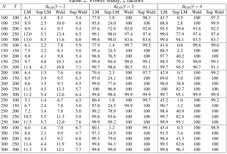
Table 1 reports the empirical sizes (in percentages) for the LM/Wald tests and Sup-LM/Wald tests (in brackets) using 5% critical values for sample sizes (N andT) equal to 100, 150, 200, 250, 300 and 1000.7. We consider three cases regarding the choice of the number of factors to be estimated by PC: (i) the correct one (¯r=r=3), (ii) smaller than the true number of factors (¯r=2<r=3),and (iii) larger than the true number of factors (¯r=4>r=3).8

Broadly speaking, the LM and Wald tests are slightly undersized forr=2 and 3 and more so when r =4. Yet the effective sizes converge to the nominal size as N and T

7_{As mentioned earlier, the critical values of the Sup–type tests are taken from Andrews (1993).}

8_{Notice that the choice ofr=3 allows us to analyze the consequences of performing our proposed test}

increase This finite sample problem is more accurate with the Sup-LM test especially for smallT, in line with the findings in other studies (see, Diebold and Chen, 1996) This is hardly surprising because, for instance, whenT =100 andΠ= [0.15,0.85], we only have 15 observations in the first subsample. By contrast, the Sup-Wald test is too liberal for

T =100. Therefore, although we impose that√T/N goes to zero, a largeT is preferable when the Sup-LM test is used. Another conclusion to be drawn is that, despite some minor differences, the tests perform quite similarly in terms of size even when the selected number of factors is not correct.

5.2

Power properties

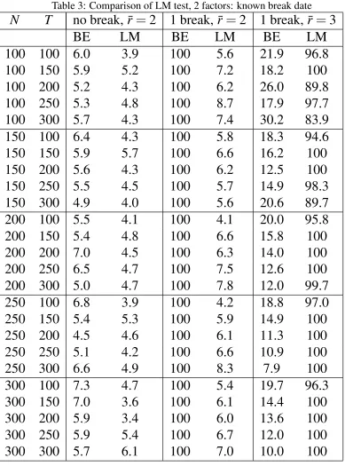
We next consider similar DGPs but this time with r=2 and now subject to big breaks which are characterized as deterministic shifts in the means of the factor loadings9. The factors are simulated as AR(1) processes with coefficients of 0.8 for the first factor and 0.2 for the second. The shifts in the loadings are 0.2 and 0.4 at timeτ =T/2. Table 2 reports the empirical rejection rates of the LM/Wald and Sup-LM/Wald tests in percentage terms using again 1000 replications.

As expected, both tests are powerful to detect the breaks as long asr=2<r¯_≤r+k1=

4, while the power is trivial when ¯r=r=2. Moreover, the power is low for the Sup-LM test whenT _≤150, which is not surprising given that the Sup-LM test is undersized. This problem could be fixed by either using size-corrected critical values, or by the Sup-Wald test that is more powerful in finite samples. For safety, we recommend to use data sets with largeT (at least around 200) in practice.

5.3

Comparison with BE test

To compare our test to the BE test, we need to construct a pooled statistic as suggested at the beginning of this section. The pooled BE test is constructed as follows:

∑N

i=1si−Nr¯

√

2Nr¯

where si is the individual LM statistics in BE (2010). This test should converge to a standarised normal distribution as long aseit andejt are independent, an assumption we also adopt here. For simplicity, we only report results for the case of known break dates.

We first generate factor models withr=2, and compare the two tests under the null. The DGPs are similar to those used in the size study. The second column of Table 3 (no break) reports the 5% empirical sizes. In general, we find that the pooled BE and the LM tests exhibit similar sizes.

Then, we generate a break in the loadings of the first factor while the other parts of the models remain the same as in the DGP where we study the power properties. The break

is generated as a shift of 0.1 in the mean of the loadings. We consider two cases: (i) the number of factors is correctly selected: ¯r=r=2; and (ii) the selected number of factors is larger than the true one: ¯r=3>r=2. The third and fourth columns in Table 3 report the empirical rejection rates of both tests. In agreement with our previous discussion, the differences in power are striking: when ¯r=2,the pooled BE test is much more powerful while the opposite occurs when ¯r=3. However, according to our result in Proposition 2, the use of Bai and Ng’s (2002) selection criteria will yield the choice of ¯r=3 as a much more likely outcome asNandT increase.

5.4

The effect of big breaks on forecasting

Finally, in this section we consider the effect of having big breaks in a typical forecasting exercise where the predictors are estimated common factors. First, we have a large panel of dataXt driven by the factorsFt which are subject to a break in the factor loadings:

Xt=AFtI(t≤τ) +BFtI(t>τ) +et

Secondly, the variable we wish to forecastyt , which is excluded from toXt, is assumed to be related toFtas follows:

yt+1=a′Ft+vt+1

We consider a DGP whereN=100,T =200,τ=100,r=2,a′= [1 1],Ftare generated as two AR(1) processes with coefficients 0.8 and 0.2, respectively,etandvtare i.i.d normal variables, and the break size is characterized by a mean shift between loadingsA andB

occuring at half of the time sample size.

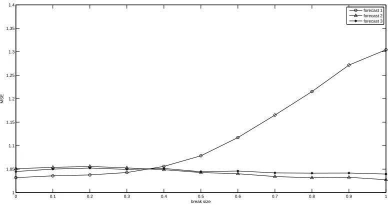
The following forecasting methods are compared in our simulation:

Bechmark Forecasting: The factorsFt are treated as observed and are used directly

as predictors. The one-step-ahead forecast ofyt is defined asyt(1) =aˆ′Ft, where ˆais the OLS estimate ofausingyt+1andFt.

Forecasting 1: We first estimated 2 factors ˆFt fromXt by PCs, which are then used as

predictors.yt(1) =aˆ′Fˆt, where ˆais the OLS estimate ofausingyt+1and ˆFt.

Forecasting 2: We first estimated 2 factors ˆFtfromXtby PC, then use ˆFtand ˆFtI(t>τ) as predictors.yt(1) =aˆ′[Fˆt FˆtI(t>τ)], where ˆais the OLS estimate ofain the regression ofyt+1on ˆFt and ˆFtI(t>τ)].

Forecasting 3: We first estimated 4 factors ˆFt fromXt by PC, then use them as

predic-tors. yt(1) =aˆ′Fˆt, where ˆais the OLS estimate ofausingyt+1and ˆFt.

The above forecastings are implemented recursively, e.g., at each time t, the data

Xt,Xt−1, . . . ,X1 and yt,yt−1, . . . ,y1 are treated as known to forecast yt+1. This process

starts fromt=149 tot =199, and the mean square errors (MSEs) are calculated by

MSE=

199

∑

t=149

(yt+1−yt(1))2 51

The results of 1000 replications are reported in Figure 1 with different break sizes rang-ing from 0 to 1. It is clear that the MSE of the Forecastrang-ing 1 method increases drastically with the size of the breaks. The Forecasting 1 and 2 procedures perform equally well and their MSEs remain constant as the break size increases, although they can not outperform the benchmark forecasting due to the estimation errors of the factors.

6

Empirical Applications

To provide a few empirical applications of our test, we first use the dataset of Stock and Watson (2009). This data consist of 144 quarterly time series for the US ranging from 1959:Q1 to 2006:Q4, concerning nominal and real variables. Since not all variables are available for the whole period, we end up using their suggested balanced panel of stan-darized variables withT =190,N=109 which more or less corresond to the case where T=200, N=100 in Table 2, where no severe size distortions are found. We refer to Stock and Watson (2009) for the details of the the data description and the standardization pro-cedure to achieve stationarity.

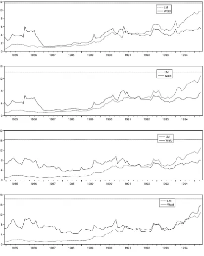
Since the estimated numbers of factors using various Bai and Ng’s (2002) information criteria range from 3 to 6, we implement the test for ¯r=3,4,5 and 6. For the Sup- LM and Wald tests, the trimmingΠ= [0.3,0.7]is used. It corresponds to the time period ranging from 1973Q3 to 1992Q3 which includes several relevant events like, e.g., the second oil price shock (1979) and the beginning of great moderation (1984). The graphs displayed in Figure 1 are the series of LM and Wald tests for different values of ¯r, with the horizontal lines representing the 5% critical values of the Sup-type test.

As can be observed, the LM and the Wald tests reject the null of no big breaks (i.e., exceeds the lower horizontal line) for ¯r=4,5,6 when the break date is assumed to be known at 1984 in agreement with the results in BE (2010). Stock and Watson (2009) get similar conclusions about the existence of breaks around the early 1980s. However, one important implication of our results is that the breaks should be interpreted as being big and thus cannot be neglected.

As for the case when the break date is not assumed to be a priori known, we find that, while the Sup-LM test cannot reject the null for all values of ¯r, the Sup-Wald test rejects the null when ¯r=5,6.(i.e., exceeds the upper horizontal line) The estimate of the break date provided by the last test is around 1979 (second oil price shock), rather than 1984 which, as mentioned before, is the only date considered by BE (2010) as a potential break date in their empirical application using the same dataset.

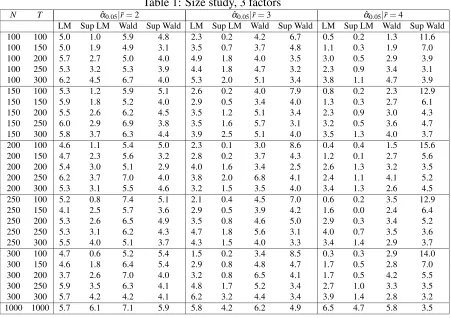
It is clear that, under the assumption of a known break date, the comparison of the test values to the 5% critical values of a χ2 distribution implies that we can easily reject the null of no big break around 1994. However, in contrast to the Stock and Watson’s (2009) dataset, if we compare the maximum of the LM and Wald tests to the critical values of the Sup-type test, no big break is detected during the sample period.

7

Conclusions

In this paper, we propose a simple two- step procedure to test for big structural breaks in the factor loadings of large dimensional factor models.that overcomes some limitations in other available tests, like Breitung and Eickmeier (2010). In particular, we derive the limiting distributions of our test, while theirs remains unknown, and show that it has much better power than their test when the choice of the number of factors is based upon Bai and Ng’s (2002) consistent information criteria Our method can be easily implemented in practice either when the break date is considered to be known or unknown, and can be adapted to a sequential procedure when the number of factors might not be correctly chosen in finite samples. Lastly, and foremost, our testing procedure is useful to avoid serious forecasting/estimation problems in standard econometric practices with factors, like FAR and FAVAR models, especially if the number of factor is a priori determined and the factor loadings are subject to big breaks.

In the second step of our testing approach, a Sup-type test is used to detect a break of the parameters in that regression when the break date is assumed to be unknown. As the simulations show, this test does not perform very well especially whenT is not too large (T<200). As other studies on the size of sup-type tests suggest, bootstrap can improve the finite sample performance of the test.compared to the tabulated asymptotic critical values of Andrews (1993). It is high in our research agenda to explore this possibility.

Further research is also needed if we were to allow for multiple breaks. As Breitung and Eickmeier point out, sequential estimation, as in Bai and Perron (1998), or an efficient search procedure, as in Bai and Perron (2003), for finding the candidate break dates may be employed.

Appendix

A.1: Proof of Propositions 1 and 2

The proof procedes by showing that the errors, factors and loadings in model (6) satisfy Assump-tions A to D of Bai and Ng (2002). Then, once this is shown, ProposiAssump-tions 1 and 2 just follow immediately from Theorems 1 and 2 of Bai and Ng (2002). DefineF_t∗= [F_t′ G_t1′]′_,εt=HGt

2+et,

Γ= [A Λ].

Lemma 1. E_||F_t∗_||4<∞and T−1∑T_t=1F_t∗F_t∗′ _→Σ_F∗ as T_→∞for some positive matrixΣ∗_F.

Proof. E_||F_t∗_||4<∞follows fromE_||Ft||4<∞by Assumption 2 and the definition ofGt1.

To prove the second part, we partition the matrixΣF(=limT→∞T−1∑Tt=1FtFt′) into:

Σ

11 Σ12

Σ′

12 Σ22

whereΣ11=limT→∞T−1∑Tt=1Ft1F1

′

t ,Σ22=limT→∞T−1∑tT=1Ft2F2

′

t ,Σ12=limT→∞T−1∑tT=1Ft1F2

′

t ,

andF_t1is thek1×1 subvector ofFt that has big breaks in their loadings,Ft2is thek2×1 subvector ofFt that doesn’t have big breaks in their loadings. By the definition ofFt∗andG1t we have:

T−1

T

∑

t=1

F_t∗F_t∗′=  

T−1∑T_t=1F_t1F_t1′ T−1∑T_t=1F_t1F_t2′ T−1∑_tT_=τ+1F_t1F_t1′ T−1∑T_t=1F_t2F_t1′ T−1∑T_t=1F_t2F_t2′ T−1∑_tT_=τ+1F_t2F_t1′ T−1∑T_t=τ+1F_t1F_t1′ T−1∑_tT_=τ+1F_t1F_t2′ T−1∑_tT_=τ+1F_t1F_t1′

 

By Assumption 2, the above matrix converges to

Σ∗ F=

 

Σ11 Σ12 (1−π∗)Σ11

Σ′

12 Σ22 (1−π∗)Σ′12

(1₋π∗)Σ11 (1−π∗)Σ12 (1−π∗)Σ11

 

Moreover,

det(Σ∗_F) =det  

Σ11 Σ12 0

Σ′

12 Σ22 (1−π∗)Σ′12 0 0 π∗(1₋π∗)Σ11



=det(ΣF)det(π∗(1−π∗)Σ11)>0

becauseΣF is positive definite by assumption. This completes the proof.

Lemma 2. E_||Γi||4<∞, and N−1Γ′Γ→ΣΓas N →∞for some positive definite matrixΣΓ.

Proof. This follows directly from Assumptions 1.a and 3.

The following lemmas involve the new errors εt. LetM and M∗ denote some positive

con-stants.

Lemma 3. E(εit) =0, E|εit|8≤M∗

Proof. This follows easily fromE_|eit|8≤M(Assumption 4),E(Ft) =0,E||Ft||4<∞(Assumption

Lemma 4.E(ε′

sεt/N) =E(N−1∑iN=1εisεit) =γN∗(s,t),|γN∗(s,s)| ≤M∗for all s, and∑Ts=1γN∗(s,t)2≤

M∗for all t and T .

Proof.

γ∗

N(s,t) = N−1 N

∑

i=1

E(εisεit)

= N−1

N

∑

i=1

E(eis+ηi′G2s)E(eit+ηi′Gt2)

= N−1

N

∑

i=1

E(eiseit) +E(ηi′G2sηi′G2t)

≤ N−1

N

∑

i=1

E(eiseit) +N−1 N

∑

i=1

q

E η_i′G2

s

2

E η_i′G2t

2

SinceN−1∑N_i=1E(eiseit) =γN(s,t)by Assumption C of Bai and Ng (2002), andE ηi′G2t

2

=O(_NT1 ) for alltby Assumptions 1.b and 2, we haveγ_N∗(s,t)_≤γN(s,t) +O(_NT1 ). Then

|γN∗(s,s)| ≤ |γN(s,s)|+O(

1

NT)≤M

∗

by Assumption C of Bai and Ng (2002). Moreover,

T

∑

s=1

γ∗

N(s,t)2 ≤ T

∑

s=1

γN(s,t) +O(

1

NT)

2

=

T

∑

s=1

γN(s,t)2+O(

1

N)

≤ M+O(1

N)≤M

∗

by Assumption E.1 of Bai (2003). The proof is complete.

Lemma 5. E(εitεjt) =τi j∗,t with|τi j∗,t| ≤ |τi j∗|for someτi j∗ and for all t; and N−1∑Ni=1∑Nj=1|τi j∗| ≤

M∗.

Proof. By Assumption C.3 of Bai and Ng (2002),_|τi j,t| ≤ |τi j|for someτi jand allt, whereτi j,t =

E(eitejt). Then:

|τˆi j,t| = |E(εitεjt)|

= _|E(eit+ηi′Gt2)(ejt+η′jG2t)|

≤ |E(eitejt)|+

q

E η_i′G2

s

2

E η_i′G2t

2

≤ |τi j|+O(

1

NT)

for allt. Therefore

N−1

N

∑

i=1

N

∑

j=1

|τi j∗| ≤ N−1 N

∑

i=1

N

∑

j=1

|τi j|+O(

1

NT)

≤ M+O(1

T)

by Assumption C.3 of Bai and Ng (2002).

Lemma 6. E(εitεjs) =τi j∗,tsand(NT)−1∑Ni=1∑Nj=1∑Tt=1∑Ts=1|τi j∗,ts| ≤M∗.

Proof. By Assumption C.4 of Bai and Ng (2002),(NT)−1_∑N

i=1∑Nj=1∑Tt=1∑Ts=1|τi j,ts| ≤M, where

E(eitejs) =τi j,ts. Then:

E(εitεjs) =τi j∗,ts=E(eitejs) +E(ηi′Gt2η′jG2s) =τi j,ts+E(ηi′G2tη′jG2s)

and we have

(NT)−1

∑

i=1

N

∑

j=1

T

∑

t=1

T

∑

t=1

|τi j∗,ts| ≤ (NT)−1 N

∑

i=1

N

∑

j=1

T

∑

t=1

T

∑

t=1

|τi j,ts|+ (NT)−1 N

∑

i=1

N

∑

j=1

T

∑

t=1

T

∑

t=1

|E(η_i′G_t2η′_jG2_s)_|

≤ M+O(1)

≤ M∗

following the same arguments as above.

Lemma 7. For every(t,s), E_|N−1/2∑N_i=1[εisεit−E(εisεit)]|4≤M∗.

Proof. Sinceεit=eit+ηi′Gt2=eit+Op(√1_NT), we have:

E_|N−1/2

N

∑

i=1

[εitεis−E(εitεis)]|4 = E|N−1/2 N

∑

i=1

[eiteis−E(eiteis) +Op(

1

√

NT) +O(

1

√

NT)]|

4

= E_|N−1/2

N

∑

i=1

[eiteis−E(eiteis)] +Op(

1

√

T) +O(

1

√

T)|

4

≤ M+O(√1

T)

≤ M∗

Lemma 8. E

1

N∑ N i=1

1 √ T∑ T t=1Ft∗εit

2

≤M∗. Proof. By the definition ofεit we have:

E

1

N

N

∑

i=1

1 √ T T

∑

t=1

F_t∗εit

2 ≤E 1 N N

∑

i=1

1 √ T T

∑

t=1

F_t∗eit

2 +E 1 N N

∑

i=1

1 √ T T

∑

t=1

F_t∗η_i′G2_t

2

then by the definition ofF_t∗andG2_t,

1 √ T T

∑

t=1

F_t∗eit

2 = 1 √ T T

∑

t=1

Fteit

2 + 1 √ T T

∑

t=τ+1

F_t1eit

2 1 √ T T

∑

t=1

F_t∗η_i′G2_t

2 = 1 √ T T

∑

t=1

Ftηi′Ft2

2 + 1 √ T T

∑

t=1

F_t1η_i′F_t2

2

Therefore, by Assumptions 1.b, 2 and 5, it follows easily that the first part of the right hand side of the last inequality isO(1)and the second part isO(_N1). Thus the proof is complete.

Once we have proved that the new factors: F_t∗, the new loadings: Γand the new errors: εt all