Around the world with Irving Fisher

BIROn - Birkbeck Institutional Research Online

Gylfason, T. and Tómasson, H. and Zoega, Gylfi (2016) Around the world

with Irving Fisher. The North American Journal of Economics and Finance

36 , pp. 232-243. ISSN 1062-9408.

Downloaded from:

Usage Guidelines:

Please refer to usage guidelines at or alternatively

18 November 2015.

Around the World with Irving Fisher

Thorvaldur Gylfason,* Helgi Tómasson,** and Gylfi Zoega***

Abstract

This paper aims to show why Irving Fisher’s own data on interest rates and inflation in New York, London, Paris, Berlin, Calcutta, and Tokyo during 1825-1927 suggested to him that nominal interest rates adjusted neither quickly nor fully to changes in inflation, not even in the long run. In Fisher’s data, interest rates evolve less rapidly than inflation and change less than inflation over time. Even so, the “Fisher effect” is commonly defined as a point-for-point effect of inflation on nominal interest rates rather than what Fisher actually found: a persistent negative effect of increased inflation on real interest rates.

Keywords: Fisher effect, inflation, interest rates.

JEL Classification: E31, E43.

*_{Professor of Economics, University of Iceland, 101 Reykjavik; tel: +3545254500; email: gylfason@hi.is.} ** _{Professor of Statistics, University of Iceland.}

1

1. Introduction

We use modern empirical methods to estimate the time series properties of nominal interest rates, real interest rates and inflation and the relationship between these variables using Irving Fisher’s (1930) data on interest rates and inflation collected from six financial centers around the world. In particular, we explore the empirical validity of the so-called Fisher effect or hypothesis which states that inflation affects the nominal rate of interest one-for-one leaving the real rate of interest unchanged.1

Fisher’s (1930) data suggest, as we will show, that nominal interest rates do not mirror the movements in inflation, even in the long run. Fisher (1930, 413) recorded “a great

unsteadiness in real interest when compared with money interest,” and attributed this result to money illusion. Therefore, it is more fitting to define the Fisher hypothesis as referring to a theoretical possibility arising from the Fisher equation and the assumption of rational expectations, what Fisher called “foresight,” rather than as referring to his empirical results.2

2. Historical Context

Many writers continue to attribute to Fisher the idea that real interest rates are immune to changes in inflation and to suggest that Fisher thought it somehow natural for real interest rates to be so immune. For example, Okun (1981, 208) states: “As Fisher saw it, an extra 1 percentage point of expected inflation raises the nominal expected rate of return on real capital assets by 1 percentage point and induces a parallel increase of 1 percentage point in bond and bill yields to keep expected returns in balance.” For another example, using quarterly U.S. data for 1954-1969, Feldstein and Eckstein (1970, 366) write: “The data thus confirm the two basic Fisherian hypotheses: (1) in the long run, the real rate of interest is (approximately) unaffected by the rate of inflation, but (2) in the short run, the real rate of interest falls as the rate of inflation increases.” 5

The Fisher effect – through which nominal interest rates react to changes in inflation point by point so as to leave real interest rates unchanged, at least in the long run – is a misnomer if described as an empirical relationship because, as will be shown here, Fisher’s (1930) own data on interest rates and inflation that he collected from six financial centers around the

1 _{See, e.g., Romer (2012, 516): “The hypothesis that inflation affects the nominal rate one-for-one is known as} the Fisher effect; it follows from the Fisher identity and the assumption that inflation does not affect the real rate.” Blanchard et al. (2010, 565) define the Fisher effect as “The proposition that, in the long run, an increase in nominal money growth is reflected in an identical increase in both the nominal interest rate and the inflation rate, leaving the real interest rate unchanged.”

2

world suggest that nominal interest rates do not come close to mirroring the movements in inflation, even in the long run. These results are consistent with those of Fisher himself. As Tobin (1987) and Dimand (1999), among others, point out, both Fisher’s theory of interest and his reading of the historical record suggested to him that real interest rates varied inversely with inflation, and that the adjustment of nominal interest rates to changes in inflation took a very long time (Fisher, 1896). In Fisher’s (1930, 43) words: “… when prices are rising, the rate of interest tends to be high but not so high as it should be to compensate for the rise; and when prices are falling, the rate of interest tends to be low, but not so low as it should be to compensate for the fall.”6

We demonstrate that Irving Fisher has suffered similar treatment as David Ricardo when different authors attach his name to an empirical relationship, not just the theoretical

proposition. Ricardian equivalence, as you know, refers to the idea that government budget deficits do not matter because taxpayers are indifferent between debt-financed and tax-financed government expenditure: they realize that current debt needs to be serviced through future taxation and plan their saving accordingly. However, the attribution of this proposition to David Ricardo is unfair to him because, even if he exposited the logic behind it, he found the proposition unconvincing.7 This short paper is intended to demonstrate anew that Ricardo is not alone, for Irving Fisher has suffered a similar treatment by his followers.

3. Fisher’s Data from Six Cities: A Time Series Approach

In an Appendix to his Theory of Interest (1930, 520-5), Fisher tabulates nominal interest rates as well as wholesale commodity price indices in six financial centers: New York, London, Paris, Berlin, Calcutta, and Tokyo, for a period spanning up to a hundred years from 1825 to 1927.8 During this period, for decades on end, prices in New York, London, and Berlin rose by merely a fraction of a percentage point per year while prices actually fell on average in Paris. Meanwhile, prices in Calcutta and Tokyo increased by 2.1 per cent and 3.9 per cent per year on average (Figure 1). Fisher’s informal analysis of the data confirmed his view that nominal interest rates tended to adjust only partially and slowly to changes in inflation, but he

6 _{Fisher (1930, 494) describes the relationship between interest rates and inflation also thus: “When the price} level falls, the rate of interest nominally falls slightly, but really rises greatly and when the price level rises, the rate of interest nominally rises slightly, but really falls greatly.” Here Fisher means the rate of change of the price level even if he says only “price level.” Fisher (1907, 270) made a clear distinction between the two: “Falling prices are as different from low prices as a waterfall is from sea level.”

7 _{To quote from Ricardo (1817, 254): “… it must not be inferred that I consider the system of borrowing as the} best calculated to defray the extraordinary expenses of the State. It is a system which tends to make us less thrifty – to blind us to our real situation.”

3

squeezed less juice out of the data than he might have. Abstracting from the cyclical fluctuations apparent in Figure 1, the Hodrick-Prescott-filtered series shown in Figure 2 confirm the impression conveyed by Figure 1 of stable nominal interest rates that most of the time exceed the considerably more variable rates of inflation.

We start the econometric analysis by studying correlations across Fisher’s data after removing trends and cycles from each time series yt with an AR(2) model, either by estimating

(1) 𝑦_𝑡 = 𝛼 + 𝛽𝑡 + 𝜙₁𝑦_𝑡−1+ 𝜙₂𝑦_𝑡−2 + 𝜀_𝑡

or

(2) Δ𝑦𝑡 = 𝛼𝑑+ 𝜙1∗Δ𝑦𝑡−1+ 𝜙2∗Δ𝑦𝑡−2+ 𝜖𝑡

We interpret the estimated residuals 𝜀_𝑡and 𝜖_𝑡 as the prewhitened versions of the original time series, and use them to study the magnitude and duration (i.e., cycle length) of the innovations in each series as well as their lead-lag structures and correlations across countries. The

estimated AR parameters are used to calculate cycle length of the series ytand yt,

respectively. The units of yt are in percentage points and the units of yt in yearly difference in percentage points.

Table 1. Cycle Length of Interest Rates and Inflation Rates 1825-1927 and Unit Root Tests

AR(2) model (1) (Years)

AR(2) model (2) (Years)

Augmented Dickey-Fuller unit root test (Intercept, lag = 2) Nominal

interest rate

Inflation rate

Nominal interest rate

Inflation rate

Nominal interest rate

Inflation rate

New York Long Long 3.3 3.1 -2.37 -3.46

London 17.7 8.1 3.5 3.1 -4.05 -4.98

Paris 8.1 4.2 3.9 3.2 -3.95 -3.45

Berlin 9.4 5.4 3.4 3.2 -3.39 -4.51

Calcutta 12.3 4.9 2.8 3.5 -5.12 -4.38

Tokyo 8.1 Long 4.1 Long -2.54 -3.58

Source: Authors’ computations based on Fisher’s data.

Note: Cycle lengths in the first four columns are measured in years. The critical value for the ADF test in the last two columns is -2.9 throughout.

4

inflation in Tokyo. With the possible exception of the interest rate series in New York and Tokyo, the ADF test results for unit roots do not suggest that detrending the series with Model 2 is better than using Model 1 (the 0.05 critical value is -2.9 throughout). The AD test results for yt in Table 1 do not suggest that detrending with Model 2, i.e., using the first difference of the series rather than using a deterministic trend, is better than Model 1. All series reflect

near-stationarity behavior, although the ADF values for New York and Tokyo are not

significant at the 5% level. Both New York and Tokyo exhibit extreme values near the end of the sample as does London (Figure 1). Because several of the series are quite short (about 40-50 years in New York, Paris, Berlin, and Tokyo), the cycle lengths shown in Table 1 cannot be very precisely estimated. A cycle in levels of, say, inflation, is not the same as a cycle in the yearly change in inflation. It is, therefore, natural to expect different cycle lengths in models of type 1 and type 2. Cycle lengths for changes in interest rates and inflation are remarkably similar across countries.

The cycle lengths shown in Table 1 are rather similar. Merging the series into an unbalanced panel offers a way of estimating a common dynamic structure for all six cities combined by detrending the data for each city by 𝜇𝑖+ 𝛽𝑖𝑡:

(3) 𝑦_𝑖,𝑡− (𝜇_𝑖+ 𝛽_𝑖𝑡) = 𝜑₁{𝑦_{𝑖,𝑡−1}− [𝜇_𝑖+ 𝛽_𝑖(𝑡 − 1)]} + 𝜑₂ {𝑦_{𝑖,𝑡−2}− [𝜇_𝑖 + 𝛽_𝑖(𝑡 − 2)]} + 𝑒_𝑡

Estimation of equation (3) suggests a cycle of 5.9 years for inflation and 16.7 years for nominal interest rates with asymptotic standard errors of 0.11 years for inflation and 29 years for interest rates. The cyclical tendency is clear for inflation, but vague for interest rates. This suggests that the dynamics of inflation and interest rates are quite different in Fisher’s data with a possible cycle in interest rates that is much longer than the inflation cycle. If a common shock sets both series in upward motion, inflation will start to descend while nominal interest rates keep rising albeit modestly, reaffirming Fisher’s view of the lack of sensitivity of nominal interest rates to inflation.

Table 2. Cross-country Correlations of Prewhitened Interest Rates 1825-1927

New York London Paris Berlin Calcutta Tokyo

New York 1.00 0.43 0.68 0.38 -0.15 -0.32

London 1.00 0.76 0.75 0.35 -0.16

Paris 1.00 0.66 -0.20 -0.21

Berlin 1.00 0.38 -0.07

Calcutta 1.00 0.13

Tokyo 1.00

5

Table 2 shows the simultaneous correlations among Fisher’s annual interest-rate series prewhitened by Model 1 (Model 2 gives similar results not shown). For New York, Fisher reports short 60-90 day commercial paper rates for 1866-1922 and long 4-6 month rates for 1890-1927; we report the former. For London, Paris, and Berlin, he reports market rates and bank rates (the London bank rate is the discount rate of the Bank of England); we report the market rates. For Calcutta and Tokyo, he reports bank rates and market rates, respectively. The shaded part of Table 2 suggests the pull of gravity: the contemporaneous correlations among interest rates within Europe and across the Atlantic are higher than those between Europe or the United States and Asia. The correlations among the European countries range from 0.66 to 0.76 compared with 0.13 between Calcutta and Tokyo. The correlations across the Atlantic range from 0.38 to 0.68. The correlations between Europe and Asia range from negative to 0.38 whereas across the Pacific, they are robustly negative. The pattern is clear: from 1825 to 1927, financial market integration was inversely related to the distance between the financial centers.

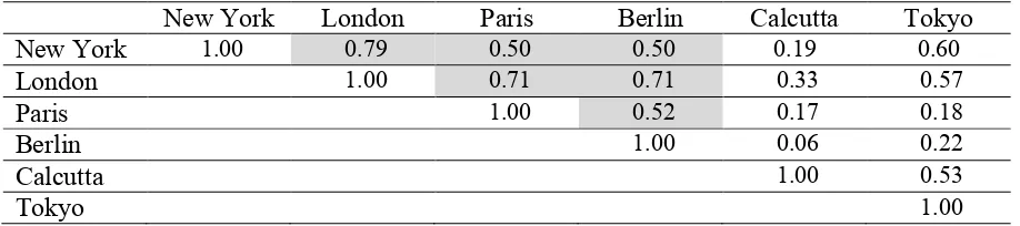
Similarly, Table 3 shows the simultaneous correlation between domestic and foreign inflation – a sign of product market integration – to vary inversely with distance. Foreign trade was free. On the whole, inflation shocks are more closely correlated across countries than interest-rate shocks. No country is seen to lead neither inflation nor interest rates. Rather, the shocks are virtually simultaneous year by year.

Table 3. Cross-country Correlations of Prewhitened Inflation Rates 1825-1927

New York London Paris Berlin Calcutta Tokyo

New York 1.00 0.79 0.50 0.50 0.19 0.60

London 1.00 0.71 0.71 0.33 0.57

Paris 1.00 0.52 0.17 0.18

Berlin 1.00 0.06 0.22

Calcutta 1.00 0.53

Tokyo 1.00

Source: Authors’ computations based on Fisher’s data.

6

To trace the reaction of nominal interest rates to inflation over time, we estimated a vector-autoregressive model (VAR with lag = 2 and a trend) for each of Fisher’s series (not shown). The impulse response functions thus obtained for London suggest that the initial (i.e.,

concurrent) correlation of 0.30 shown in Table 4 rises to 0.55 in the following year, and then gradually declines to zero in six years (Figure 3, upper panel). A higher nominal interest rate is followed by less inflation, a correlation that peters out after five years (Figure 3, lower panel). Further, Figure 3 confirms that inflation is more volatile than nominal interest rates. Increased inflation makes nominal interest rates edge upward, an effect that persists even after inflation reverses course.

Table 4. Correlations of Prewhitened Inflation and Interest Rates 1825-1927

New York London Paris Berlin Calcutta Tokyo Model 1 0.12

(0.19)

0.30* (0.001)

0.41* (0.004)

0.28* (0.02)

0.33* (0.004)

-0.11 (0.25)

Model 2 0.06 (0.33)

0.22* (0.01)

0.31* (0.02)

0.25* (0.04)

0.36* (0.002)

-0.18 (0.14) Source: Authors’ computations based on Fisher’s data.

Note: p-values are shown within parentheses. An asterisk denotes statistical significance at the 0.05 level in a one-tailed test.

Because the time series are of uneven length and short except for London, we also estimated a VAR model with country-specific trends and common dynamic AR(2) parameters. The resulting impulse response functions for all six cities combined are similar to those for London shown in Figure 3, and are more precisely estimated because the pooled sample is much larger than that for London alone. In either case, the impulse response pattern means that an increase in the inflation rate by one per cent is followed by an increase in nominal interest rates by 0.03 per cent in the first year, an effect that gradually declines to zero after six years. The pattern of interaction between nominal interest rates and inflation observed in Figure 3 suggests that interest rates are not influenced by inflation alone, and that inflation is not influenced by interest rates alone.

4. Back to Fisher: Regression Analysis

7

adaptive expectations.9 In either case, the dynamic relationship between the levels of i and can be described by a lagged dependent variable:

(4) 𝑖 = 𝑎𝜋 + 𝑏𝑖−1+ 𝑐 + 𝑒

The short-run effect of  on i is a > 0, the long-run effect is a/(1-b) > a if 1 > b > 0, the mean lag is a/(1-b)2, c is a constant reflecting a risk premium plus the price of time, and e is white noise.

Table 5. Six Cities: Regression Results on Interest Rates 1825-1927

Constant Short-run effect

Long-run effect

Mean lag (years)

Adjusted R2

New York 1867-1922

1.902

(0.698) (0.020) 0.018 (0.064) 0.050 (0.214) 0.139 0.331

London 1825-1927 1.432 (0.303) 0.050* (0.012) 0.117* (0.041) 0.276* (0.140) 0.337 Paris 1873-1914 0.795 (0.298) 0.053* (0.018) 0.170 (0.097) 0.559 (0.499) 0.492 Berlin 1862-1912 1.969 (0.433) 0.034* (0.017) 0.058* (0.029) 0.098 (0.059) 0.232 Calcutta 1862-1926 3.71 (5.64) 0.036* (0.013) 0.055* (0.023) 0.085* (0.043) 0.185 Tokyo 1888-1926 3.497 (1.013) -0.012 (-0.014) -0.025 (0.027) -0.054 (0.058) 0.327

Note: An asterisk denotes statistical significance at the 0.05 level. Standard errors are shown within parentheses. The standard errors of the estimates of the long-run effects and the mean lags are approximated by a Taylor expansion of 𝐽_𝑓𝑇_{(𝑎̂, 𝑏̂)𝐶𝑜𝑣(𝑎̂, 𝑏̂)𝐽}

𝑓(𝑎̂, 𝑏̂) where for the long-run effect

𝐽_𝑓(𝑎, 𝑏) = [1 (1 − 𝑏), 𝑎 (1 − 𝑏)_{⁄ ⁄} 2_{] and for the mean lag 𝐽}

𝑓(𝑎, 𝑏) = [1 (1 − 𝑏)⁄ 2, 2𝑎 (1 − 𝑏)⁄ 3].

For comparison with the correlations shown in Table 4, Table 5 shows OLS estimates of six such equations, one for each of Fisher’s six cities.10 With the possible exception of New York and Tokyo, the hypothesis that the interest-rate series have unit roots can be rejected

everywhere in an Augmented Dickey-Fuller test, with an intercept and a two-period lag (Table 1). Like in Rose (1988), none of the six inflation series have unit roots either (not shown). Therefore, Mishkin’s (1992) method of deducing a one-to-one long-run relationship between nominal interest rates and inflation from cointegration tests for a common trend in both series in some but not all industrial countries does not apply to Fisher’s data. Without

9 _{Examples of transactions cost in financial markets include the cost of setting up complicated models to guide} financial transactions and of hiring highly paid traders to conduct business.

8

serially correlated errors in London, Paris, Berlin, Calcutta, and possibly also Tokyo and without unit roots, OLS estimates of the parameters in equation (1) can be expected to be consistent but biased. Further, the AR(2) cycles observed in the inflation series in Section 2 suggest that the OLS estimates must be taken with a grain of salt.

Notice that current inflation has a significantly positive effect on interest rates in four of the six cities, all except New York and Tokyo.11 Where statistically significant, however, the short-run effect of inflation on interest rates is small, ranging from 0.03 to 0.05. The lagged effect of last year’s interest rate is significant throughout, ranging from 0.35 in Calcutta to 0.69 in Paris. Even so, the long-run effect of inflation on interest rates is significantly larger than zero only in London, Berlin, and Calcutta, and is well below one throughout, ranging from 0.05 in New York to 0.17 in Paris.

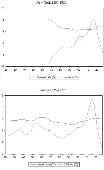
Figure 1 presents Fisher’s data on nominal interest rates and inflation, making the same point as Tables 4 and 5 by showing how real interest rates r, originally defined by Fisher (1896) as

(5) 𝑟 =_1+𝜋1+𝑖 − 1

vary inversely with inflation in Fisher’s six cities. If i adjusted fully and promptly to π, then r

would be roughly constant and independent of π. But this is not what Figure 1 shows. On the contrary, all six panels of Figure 1 suggest with a striking consistency that nominal interest rates hardly budged anywhere when inflation changed.12 This means that changes in inflation could have real effects by moving real interest rates about and thereby also investment, saving, asset portfolios, consumption, output, and employment.

In Fisher’s time, as Figure 1 shows, while inflation did not hesitate to move into negative territory, nominal interest rates did not follow. In London, wholesale prices rose merely by 9 per cent from 1820 to 1927, not per year but for the period as a whole, while in New York they remained unchanged from 1867 to 1926 as they did in Berlin from 1866 to 1911; in Paris, wholesale prices fell by 18 per cent from 1872 to 1914 (Fisher, 1930, 520-3). In Fisher’s data, deflation was nearly as common as inflation, reaffirming his inference that deflation makes both real interest rates and debt burdens rise, leading to distrust, distress selling, bankruptcies, bank runs, reduced output and trade, and unemployment (Fisher, 1896, 1933).13 There can be no controversy about deflation making real interest rates rise when

11 _{Fisher’s (1930, 532-3) quarterly data for New York 1890-1927 produce broadly similar results (not reported).} 12 _{A similar pattern of real interest rates and inflation emerges from Fisher’s quarterly data for New York} 1890-1927.

9

nominal interest rates refuse to go below zero as was the case throughout Fisher’s data. It may have been natural in those days to expect nominal interest not to follow inflation because bouts of inflation were often followed by deflation since inflation expectations were well anchored by the gold standard, but Fisher did not make this observation. In Fisher’s data, the average real interest rate as defined in equation (4) is positive everywhere over the sample period as a whole, ranging from 3.2 per cent per year in Paris to 6.1 per cent in New York.

While Fisher viewed real interest as a passive variable that varies inversely with inflation, Wicksell (1936) regarded real interest – i.e., natural interest adjusted for inflation – as the expected long-term return on new investments, arguing that an increase in the real rate of interest signaled higher profits, thus encouraging bank lending with increased inflation as a result. By suggesting an inverse relationship between inflation and real interest, Fisher’s data seem to contradict this version of Wicksell’s story. If, however, Wicksell’s real interest is viewed as money interest adjusted for inflation, Wicksell argues that an increase in money interest rates reduces inflation and increases real interest, an inverse correlation consistent with Fisher’s analysis and data.

5. More Recent Literature

Turning Fisher’s analysis of the effects of inflation on interest rates on its head, yet without invoking Wicksell’s theory, Fama (1975) postulated rational expectations

(6) 𝜋_𝑡+1 = 𝐸(𝜋_𝑡) + 𝜗_𝑡

where t+1 is the one-period-ahead inflation rate and the forecast error is orthogonal to information known at time t and where the current interest rate it mirrors expected inflation (7) 𝐸(𝜋𝑡) = 𝛼 + 𝛽𝑖𝑡+ 𝜃𝑡

if the real rate of interest is constant such that r and 1. Combining the two equations

gives

(8) 𝜋_𝑡+1 = 𝛼 + 𝛽𝑖_𝑡+ 𝜀_𝑡

If  is orthogonal to i in equation (7) and 𝜗 is orthogonal to E() in equation (6), then  is also orthogonal to i in equation (8), making the estimate of  unbiased as well as consistent

because the interest rate is measured at a point in time when inflation is not known.14 Fama reports  = 1 in U.S. data from 1954-1971. His approach requires markets to be efficient with serially random forecast errors.

10

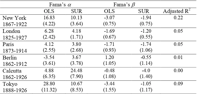
Table 6. Fama’s Test in Fisher’s Data 1825-1927

Fama’s  Fama’s 

OLS SUR OLS SUR Adjusted R2

New York 1867-1922 16.83 (4.22) 10.13 (3.64) -3.07 (0.75) -1.94 (0.75) 0.22 London 1825-1927 6.28 (2.42) 4.18 (1.71) -1.69 (0.67) -1.20 (0.55) 0.05 Paris 1873-1914 4.12 (2.55) 3.80 (2.68) -1.71 (0.93) -1.74 (1.06) 0.05 Berlin 1862-1912 -3.54 (3.61) 3.67 (3.78) 1.20 (1.05) -0.55 (1.14) 0.01 Calcutta 1862-1926 4.88 (6.35) 24.48 (7.90) -0.48 (1.08) -4.0 (1.40) 0.00 Tokyo 1888-1926 28.80 (11.32) 10.67 (8.53) -3.44 (1.55) -1.05 (1.17) 0.09

Note: Standard errors are shown within parentheses.

Table 6 shows that estimates of equation (8) with Fisher’s data for each of the six cities listed in Tables 1-5 contradict Fama’s finding, and can perhaps as well be interpreted as

11

nominal interest rates was not the source of the weak correlation between nominal interest and inflation – that is, the strong inverse correlation between real interest and inflation.

Mishkin (1984) tested for full adjustment in seven OECD countries during 1967-1979,15 and rejected the constancy of real interest rates in each case, which means that real interest rates in these countries decline with increased inflation. Mishkin (1992) reports cointegration between inflation and nominal interest rates in U.S. data, which he interprets as full

adjustment of nominal interest rates to inflation in the long run, implying that the two series will move together along trend generating a high correlation. He rejects full adjustment in the short run when the two series are stationary, concluding that short-term fluctuations in interest rates reflect macroeconomic shocks while long-term movements may reflect changes in inflation expectations.

In sum, the absence of full adjustment of nominal interest rates to inflation when inflation and interest rates are stationary is consistent with the absence of such a relationship in Fisher’s data. Fisher found the contemporaneous correlation between inflation and nominal interest rates to be weak. When he related nominal interest rates to distributed lags of past inflation rates as a proxy for the market’s expected rate of inflation, the effect remained quite weak. Fisher also proposed comparing the variance of real and nominal interest rates,

suggesting that if the former was larger than the latter then interest rates did not respond fully to inflation (recall Figure 1). As we do, Summers (1982, 26) observes that “there is no sense in which his [Fisher’s] results can be said to demonstrate the empirical validity of the theory that bears his name.”

More recent empirical evidence, surveyed by Cooray (2003), mostly supports Fisher’s findings. For example, Koustas and Serletis (1999) find no evidence of an effect of inflation on short-term interest rates. Fahmy and Kandil (2003) report a weak effect of inflation on short-term interest rates while trends in inflation and interest rates tend to coincide.

6. Discussion

In retrospect, it is clear that the name of one of the world’s great economists came should be associated only with the theoretical relationship between nominal interest rates and expected inflation in the absence of money illusion, not with the empirical validity of that relationship. Fisher’s (1930, 415) view was that “… men are unable or unwilling to adjust at all accurately or promptly the money interest rates to changed price levels. Negative real interest rates could scarcely occur if contracts were made in a composite commodity standard. The erratic

12

behavior of real interest is evidently a trick played on the money market by the “money illusion” when contracts are made in unstable money.” A few pages earlier, Fisher (1930, 400) had written: “Most people are subject to what may be called “the money illusion,” and think instinctively of money as constant and incapable of appreciation or depreciation.” Fisher understood that under certain circumstances, including perfect foresight, real interest rates might be immune to changes in inflation, at least over the long haul, but he rejected the premises needed to erect such a theory. His appeal to money illusion made him suspect, however, at a time when Keynesian economics was under siege on partly similar grounds, and triggered three reactions. Some rebelled against Fisher by applying econometric time series methods to more recent data, concluding in some cases that real interest rates were immune to inflation after all (e.g., Fama, 1975), but this approach met later with mixed success and, further, it left Fisher’s own data unexplained. Others built models showing how money illusion was not necessary to explain how changes in the rate of inflation could move real interest rates and other real magnitudes (e.g., Mundell, 1963; Tobin, 1965), for the rate of inflation, all things considered, is a relative price. Endogenous growth theory, by making also real interest rates endogenous in the long run, makes a similar point. Others still argue that money illusion is real (Akerlof and Shiller, 2009, 41-50).

7. Conclusion

13

References

Akerlof, George A., and Robert J. Shiller (2009), Animal Spirits: How Human Psychology Drives the Economy, and Why It Matters for Global Capitalism, Princeton University Press, Princeton, NJ.

Blanchard, Olivier, Alessia Amighini and Francesco Giavazzi (2010), Macroeconomics: A European Perspective, Prentice Hall.

Bordo, Michael D., and Andrew J. Filardo (2005), “Deflation in a Historical Perspective,” BIS Working Paper 186, Bank for International Settlements.

Cooray, Arusha (2003), “The Fisher Effect – A Survey,” Singapore Economic Review 48(2), 135-150.

Dimand, Robert W. (1999), “Irving Fisher and the Fisher Relation: Setting the Record Straight,” Canadian Journal of Economics 32(3), May, 744-750.

Fahmy, Yasser A. F., and Magda Kandil (2003), “The Fisher Effect: New Evidence and Implications,” International Review of Economics and Finance 12(4), 451-465. Fama, Eugene F. (1975), “Short-term Interest Rates as Predictors of Inflation,” American

Economic Review 65(3), June, 269-282.

Feldstein, Martin, and Otto Eckstein (1970), “The Fundamental Determinants of the Interest Rate,” Review of Economics and Statistics 52(4), November, 363-375.

Fisher, Irving (1896), Appreciation and Interest, AEA Publications 3(11), August, 331-442. Fisher, Irving (1907), The Rate of Interest, MacMillan.

Fisher, Irving (1930), The Theory of Interest, MacMillan.

Fisher, Irving (1933), “The Debt-Deflation Theory of Great Depressions,” Econometrica 1(4), 337-357.

Koustas, Zisimos, and Apostolos Serletis (1999), “On the Fisher Effect,” Journal of Monetary Economics 44(1), 105-130.

Mishkin Fredrick S. (1981), “The Real Rate of Interest: An Empirical Investigation,” The Cost and Consequences of Inflation, Carnegie-Rochester Conference Series on Public Policy 15, 151-200.

Mishkin, Fredrick S. (1984), “The Real Interest Rate: A Multi-Country Empirical Study,”

Canadian Journal of Economics 17, 283-311.

Mishkin, Fredrick S. (1992) “Is the Fisher Effect for Real? A Reexamination of the

14

Mundell, Robert A. (1963), “Inflation and Real Interest,” Journal of Political Economy 71, June, 280-283.

Nelson, C.R., and G.W. Schwert (1977), “Short-Term Interest Rates as predictors of Inflation: On Testing the Hypothesis that the Real Rate of Interest is Constant,” American Economic Review 67, 478-86.

Okun, Arthur M. (1981), Prices and Quantities: A Macroeconomic Analysis, Basil Blackwell, Oxford.

Romer, David (2012), Advanced Macroeconomics, 4th edition, McGraw-Hill. Rose, Andrew (1988), “Is the Real Interest Rate Stable?,“ Journal of Finance 43(5),

December, 1095-1112.

Summers, Lawrence H. (1982), “The Non-adjustment of Nominal interest Rates: A Study of the Fisher Effect,” NBER Working Paper No. 836.

Thaler, Richard H. (1997), “Irving Fisher: Modern Behavioral Economist,” American Economic Review, 87 (2), 439-441.

Tobin, James (1965), “Money and Economic Growth,” Econometrica 33(4), October, 671-684.

Tobin, James (1987), “Fisher, Irving,” The New Palgrave Dictionary of Economics, eds. John Eatwell, Murrey Millgate, and Peter Newman, 2, 369-376.

15

Figure 1. Six Financial Centers: Nominal Interest Rates and Inflation 1825-1927

New York 1867-1922

` -40 -30 -20 -10 0 10 20 30 40

20 30 40 50 60 70 80 90 00 10 20

Interest rate (%) Inflation (%)

London 1825-1927

-40 -30 -20 -10 0 10 20 30 40

20 30 40 50 60 70 80 90 00 10 20

16 Paris 1873-1914

-40 -30 -20 -10 0 10 20 30 40

20 30 40 50 60 70 80 90 00 10 20

Interest rate (%) Inflation (%)

Berlin 1862-1912

-40 -30 -20 -10 0 10 20 30 40

20 30 40 50 60 70 80 90 00 10 20

17

Calcutta 1862-1926

-40 -30 -20 -10 0 10 20 30 40

20 30 40 50 60 70 80 90 00 10 20

Interest rate (%) Inflation (%)

Tokyo 1888-1926

-40 -30 -20 -10 0 10 20 30 40

20 30 40 50 60 70 80 90 00 10 20

Interest rate (%) Inflation (%)

18

Figure 2. Six Financial Centers: Hodrick-Prescott-filtered Nominal Interest Rates and Inflation 1825-1927

New York 1867-1922

` -8 -4 0 4 8 12

20 30 40 50 60 70 80 90 00 10 20

Interest rate (%) Inflation (%)

London 1825-1927

-8 -4 0 4 8 12

20 30 40 50 60 70 80 90 00 10 20

19 Paris 1873-1914

-3 -2 -1 0 1 2 3 4 5

20 30 40 50 60 70 80 90 00 10 20

Interest rate (%) Inflation (%)

Berlin 1862-1912

-3 -2 -1 0 1 2 3 4 5 6

20 30 40 50 60 70 80 90 00 10 20

20

Calcutta 1862-1926

-8 -4 0 4 8 12

20 30 40 50 60 70 80 90 00 10 20

Interest rate (%) Inflation (%)

Tokyo 1888-1926

-8 -4 0 4 8 12

20 30 40 50 60 70 80 90 00 10 20

Interest rate (%) Inflation (%)

21

Figure 3. London: Interaction of Nominal Interest Rates and Inflation 1825-1927

Impulse responses to an inflation rate shock by one standard deviation

-1 0 1 2 3 4 5 6 7 8

0 1 2 3 4 5 6 7 8 9 10 11

Years

Response of inflation rate Response of nominal interest rate

Impulse responses to a nominal interest rate shock by one standard deviation

-2.5 -2.0 -1.5 -1.0 -0.5 0.0 0.5 1.0

0 1 2 3 4 5 6 7 8 9 10 11

Years

Response of nominal interest rate Response of inflation rate

Source: Authors’ computations. Note: The vertical axes show the response of nominal interest rates and inflation measured in standard deviations to an increase in each of those variables by one standard deviation. The