Inter dimensional effects in nano structures

N A N O E X P R E S S

Open Access

Inter-dimensional effects in nano-structures

Rainer Dick

Abstract

We report on two extensions of the traditional analysis of low-dimensional structures in terms of low-dimensional quantum mechanics. On one hand, we discuss the impact of thermodynamics in one or two dimensions on the behavior of fermions in low-dimensional systems. On the other hand, we use both quantum wells and interfaces with different effective electron or hole mass to study the question when charge carriers in interfaces or layers exhibit two-dimensional or three-dimensional behavior. We find in particular that systems with different effective masses in the bulk and in the interface exhibit separation of two-dimensional and three-dimensional behavior on different length scales, whereas quantum wells exhibit linear combination of two-dimensional and three-dimensional behavior on short length scales while the behavior on large length scales cannot be associated with either two-dimensional or three-dimensional behavior.

Keywords: Density of states, Coulomb interactions, Exchange interactions, Scattering in nano-structures, Thermal properties in nano-structures, Fermi energy in nano-structures

Background

Nano-structures traditionally provide approximate real-izations of low-dimensional systems through confined electron states in one dimension (thin films, interfaces or quantum wells), two dimensions (quantum wires or nano-wires), or three dimensions (quantum dots or color centers). We emphasize electron states rather than elec-trons in the following discussions, because for conduction bands with large filling factors or p-doped semiconduc-tors, we usually think of the unoccupied electron states as holes, which can also be confined [1-3].

In the olden days, confined electron states primarily provided dimensionally restricted realizations of electric charge carriers, but since the advent and rise of spintron-ics, low-dimensional spin systems also play an important role in nano-technology. Low-dimensional spin systems are directly linked to confined electron states because the coupling of a particle with spinSto magnetic fieldsB is proportional to inverse particle mass,

HI= − q 2mB·

M+2S

.

Correspondence: [email protected]

Department of Physics & Engineering Physics, University of Saskatchewan, 116 Science Place, Saskatoon, Saskatchewan, S7N 5E2, Canada

Here, m is the (effective) mass, and q is the charge of the particle, q = ±e for holes or electrons, respec-tively.M is the angular momentum of the particle. Low-dimensional systems in spintronics are therefore directly linked to confined electron states because electrons or holes do not only provide the lightest movable charge car-riers, but also interact stronger with magnetic fields than any other readily available (quasi-)particle in materials. Furthermore, energy gaps between different spin config-urations are determined by exchange integrals, and the spatial extent of the wave function of a bound particle of massmtypically scales with 1/m. Exchange interactions between electrons or holes can therefore align or anti-align spins, whereas inter-nuclear exchange interactions are negligible in materials science.

A well-known primary effect of a reduced number d of dimensions in nano-systems is the significant change in the energy dependence of the density of states in the energy scale, (E) ∼ √Ed−2. This directly affects the thermal and electrical conductivity properties of nano-systems and impacts the use of spins for information storage and processing. Furthermore, even without con-finement, particles can exhibit low-dimensional behavior on certain energy and length scales if their propaga-tion properties are affected by the presence of layers, interfaces, or wire-type structures in which the particles

propagate with an effective mass which is very different from their effective mass in the adjacent bulk materials [4,5].

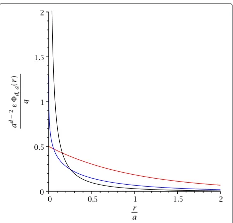
Confinement of electromagnetic fields and photons is harder to accomplish than for electrons or holes, but effects of restricted dimensionality are also striking and of high potential relevance for technology [6]. Confine-ment of electromagnetic fields changes the distance law for electric forces to|E(r)| ∼ r−(d−1) _{with the potential} for logarithmic or linear confinement of electric charges ind = 2 ord = 1, respectively. Even screened electric forces and potentials are affected, see Figure 1 [7].

Figure 1 illustrates that in lower dimensions, interac-tions are comparatively stronger at large distances and weaker at short distances. The same effect would apply for any other interaction which would be mediated by con-fined bosons; for example, it would also apply to phonon-mediated interactions between electrons or holes. The reduced interaction strength at smaller distance in lower dimensions is a consequence of the weaker singularity of the field near its source, whereas the increase in strength at larger distance intuitively can be attributed to the squeezing of field lines into a smaller number of dimen-sions. This change in distance behavior directly impacts electric forces between charges and implies the poten-tial emergence of electrical confinement in systems with dimensionally restricted electromagnetic fields. In addi-tion, it also impacts effective spin-spin interactions in spintronics because thed-dimensional electrical potential also appears in the exchange integrals which determine the energy splits between spin configurations.

Figure 1Electric potentialsd,a(r)with screening lengtha.The red curve corresponds tod=1, blue tod=2, and black tod=3.

Methods

Low-dimensional quantum mechancis with one or two-dimensional Hamilton operators, or three-two-dimensional Hamiltonians with confining boundary conditions are widely used to analyze and understand the importance of quantum effects on confined particles in nano-systems. Here, we wish to report on extensions of this analysis in two directions: (1) impacts of low-dimensional thermody-namics on the behavior of charge carriers and (2) quan-tum mechanical analysis of inter-dimensional behavior in materials with a low-dimensional component. We focus also on a thin interface or layer as the low-dimensional component, but the same methods can be applied, e.g., to analyze dimensional competition in the case of a nano-wire on a surface [8]. Inter-dimensional effects in these systems can be relevant, e.g., for charge transport in nano-wires, which attract a lot of interest, e.g., for its use in photovoltaics [9]. We will use both the method of inter-dimensional Green’s functions [4,5,10] and grand canonical ensembles in low-dimensional systems to ana-lyze impact of dimensionality of a system on the behavior of electrons and photons.

The d-dimensional fields and potentials are direct consequences of the solutions of Laplace-Poisson or Helmholtz equations in d dimensions. The pertinent properties of these solutions are generically encoded in the Green’s functions which satisfy

+2m

2E

x|Gd(E)|x = −δ(x− x) (1)

in the energy representation, or

i∂ ∂t+

2

2m

x|G(t)|x =δ(t)δ(x− x) (2)

in the time domain. The Green’s functions are related according to

x|Gd(E)|x = − 2mE

2 x|Gd(E)|x =

∞

−∞dtx|Gd(t)|x

_exp(iEt/), (3)

x|Gd(t)|x = 1 2π

_∞

−∞dEx|Gd(E)|x

_{exp(−iEt/).}

(4)

The conditions (1) and (2) do not completely specify the Green’s functions, and we impose the physical boundary conditions that the Green’s function in the region of neg-ative energyE<0 should vanish for|x− x| → ∞, while the positive energy Green’s function should describe out-going spherical waves∼ exp(ikr)/√rd−1,k = √2mE/, in the limitr= |x− x| → ∞. These conditions yield the well-known retarded Green’s functions

x|Gd(t)|x = (t) i(2π )d

ddkexpik·(x− x)

−

2m(t−i)k 2

= (t) i

m 2πi(t−i)

d exp

im(x− x ₎2

2(t−i)

(5)

in the time domain. The energy-dependent Green’s func-tions are with the notationx|Gd(E)|x ≡ Gd(x− x,E) given by

Gd(x,E)= (−E)

√ 2πd

_√

−2mE

r d−2

2 Kd−2

2

_√

−2mEr

+ iπ 2

(E) √

2πd

_√

2mE r

d−2 2

H(d1−)2 2

_√

2mEr

,

(6)

(see Appendix I in [7] for derivations). The functionsKν andHν(1)are modified Bessel functions and Hankel func-tions of the first kind, respectively, and we follow the notations and conventions of [12] for special functions.

However, if there are parameter ranges in materials and devices where electrons or photons behave according to the laws of two-dimensional or three-dimensional quan-tum mechanics and electrodynamics, then there should also exist transition regimes with intermittent dimen-sional behavior. This is the realm where particles or forces are described by theinter-dimensionalor dimen-sionally hybrid Green’s functions introduced in [4,5]. We should also point out that another important novel approach to inter-dimensional behavior in systems with low-dimensional components concerns the study of inter-dimensional universality for critical scaling laws. This notion has been introduced and studied for domain wall dynamics in nano-wires [13].

We will review the basic aspects of physics in var-ious dimensions in the section on “Green’s functions, potentials, and densities of states in d dimensions” and then discuss a lesser known but technologically relevant aspect of physics in lower dimensions, viz., the impact of dimensionality on statistical and thermal physics in low-dimensional systems, in the section on “Thermal

properties of the charge carriers in d dimensions”. We will then discuss the construction of dimensionally hybrid Green’s functions for quantum wells in the section on “Inter-dimensional effects in interfaces and thin layers”. This will also allow us to calculate the inter-dimensional density of states (E) and the relation between Fermi energy and electron density in the quantum well in the section entitled “Density of states for the thin quan-tum well”. Comparison of the results for the quanquan-tum well with the results for layers with different effective mass of charge carriers [5] or different permittivity [6] reveals that a difference in potential energy between a layer and a bulk yields linear combinations of two-dimensional and three-two-dimensional terms at the same length scales, whereas difference in kinetic terms (viz. effective mass which affects kinetic terms for electrons, holes, or permittivity, which affects the kinetic terms for photons), separates two-dimensional behavior on short length scales from three-dimensional behavior at large length scales.

Results and discussion

We can now enter into the discussion of less known results on the low-dimensional quantum and statistical physics of charge carriers and new results and observations concern-ing inter-dimensional behavior in the presence of layers or interfaces. We will separate this discussion into sub-sections on interaction potentials and thermal properties in low-dimensional fermion systems, and a subsection on inter-dimensional effects as inferred from Green’s func-tions.

Green’s functions, potentials and densities of states ind

dimensions

We have chosen the paradigm of the Green’s functions for the free Schr¨odinger equation (1,2) because it encom-passes most of the practical applications of Green’s func-tions in materials and devices. The energy-dependent Green’s function for the free Schr¨odinger equation not only describes the electron or hole scattering of impurities or the density of states in the energy scale in free elec-tron gas models, but it also describes the electric potential of a charge densityρ(x)and exchange integrals between electron states inddimensions through the zero energy Green’s function

x|Gd(E=0)|x ≡ x|Gd|x.

The Coulomb and exchange type potentials and interac-tions are given in terms of this Green’s function through

d(x)= 1

and

Jnn = e2

ddx

ddx+_n(x,t)+_n(x,t)

× x|Gd|xn(x,t)n(x,t),

(8)

respectively. Furthermore, with the substitution 2mE = −2_/a2_{, the energy-dependent Green’s function also} describes screened interaction potentials with screening lengtha,

d,a(x)= 1

ddxx|Gd(−2/2ma2)|xρ(x), (9)

− 1

a2

_d,a(x)= −1 ρ(x),

and correspondingly screened exchange interactions. Practical realization of low-dimensional Coulomb or Yukawa potentials (Equations (7) and (9) with d = 1 or d = 2) in devices may be possible with the help of photonic bandgap materials, and the two-dimensional logarithmic behavior should be realized at short distances in high permittivity thin films [6].

However, a more direct and immediate application of d-dimensional Green’s functions in materials sci-ence and device engineering concerns scattering in low-dimensional structures. Scattering of a particle of momen-tum k by a localized or screened impurity potential V(x)is described by a wave function which contains the energy-dependent Green’s function

ψ_k(x)=exp(ik· x)− 2m

2

ddxGd(x− x,2k2/2m)V(x)exp(ik· x)

=exp(ik· x)− iπm (2π )d/22

ddx

k |x− x|

d−2 2

×H(d1−)2 2

k|x− x|V(x)exp(ik· x).

(10)

This yields the differential scattering cross section ind dimensions,

dσ

d =r→∞lim r

d−1jout(k) jin(k)

=f(kxˆ− k)2, (11)

with the scattering amplitude

f(k)= − mk (d−3)/2 (2π )(d−1)/22

ddxexp(−ik· x)V(x).

(12)

The most interesting feature of this result from a nano-device point of view concerns suppressed high energy

scattering and enhanced low energy scattering from impu-rities in low dimensions roughly according todσ/d ∼ kd−3∼√Ed−3.

Another application of low-dimensional physics for nano-scale devices concerns the density of states (or num-ber of electronic orbitals) in the energy scale,

d(E)=2(E) m 2π

d √ Ed−2

(d/2)d. (13)

These are densities of states perd-dimensional volume and per unit of energy, i.e., V_d(E)dE is the number of electronic states in a d-dimensional volumeV and with energies betweenEandE+dE. The corresponding rela-tion between the Fermi energy EF and the density n of electrons inddimensions is therefore

nd=

2 d_((d+2)/2)

mEF 2π

d

. (14)

This makes physical sense: In a smaller number of dimensions, we need a larger Fermi sphere inkspace to accommodate the same electron density inxspace.

Equations (13) and (14)a priorirefer to a free electron gas model. In materials science, this is a useful approxima-tion for semi-conductors and a very good approximaapproxima-tion for metals at room temperature. For energy bands with minimal energyE0, corresponding effective massm∗, and a low filling factor, Equation (13) applies for the electron density of states with the substitutionsE → E−E0and m→m∗. For nearly filled bands with maximal energyE1, the substitutions E → E1−E,m → mhyield the hole density of states.

Densities of states are important for electrical and ther-mal transport properties of materials and for the optical properties of materials. For example, the photon absorp-tion cross-secabsorp-tion for excitaabsorp-tion of an electron from a discrete donor or quantum dot state into a continuous energy band is directly proportional to the density of final electron states. Therefore, the densities of states (13) for d = 1, 2, and 3 are common items for information in nano-technology textbooks. However, strict electron con-finement to a quantum wire or an interface is apparently a bad approximation in most cases and makes only sense for the subset of low lying energy states in deep quantum well structures. Therefore, we will revisit the density of states in the section on “Density of states for the thin quantum well” in the framework of a solvable quantum well model.

Thermal properties of the charge carriers inddimensions

the boundary conditions of given energy and particle number (if we use a grand canonical ensemble) does not depend on the number of dimensions. However, the cal-culation of partition functions and thermodynamic quan-tities from the Fermi-Dirac or Bose-Einstein distributions involvesd-dimensional integrals; therefore, thermal prop-erties of a system will depend on the number of dimen-sions in which particles can move. I would hope that the introduction in this section can serve as a brief com-pendium and overview of basic aspects of this dependence of thermal properties ond. We will find that the specific heat in particular is affected byd. Due to the particular relevance of confined fermionic charge and spin carriers for nano-technology, we will focus on low-dimensional implications of Fermi-Dirac statistics.

We can derive all the basic properties of the d-dimensional fermion gas from its grand canonical potential

= −βp= −2V

ddk (2π )dln

1+expβμ−βEk.

The approximation of an ideal non-relativistic gas,E= 2_k2_{/2m, is known to yield excellent results for metals. For} semiconductors with a low filling factor in the conduction band, we can useE=2k2/2m∗if we also calculateμand EF from the minimum of the energy band. For high fill-ing factor, we should calculate the chemical potential and Fermi energy for the holes downwards from the maximum of the energy band, of course, to useE=2_k2_/2m

h. If the density of effectively free charge carriers in a material is small, as in a semiconductor, then the ther-mal properties of the electrons or holes can be described by a non-degenerate Fermi gas. With the understanding to calculate energies and chemical potentials from the corresponding energy band extremum, the conditions for applicability of a non-degenerate Fermi gas model for the conduction electrons or holes are

EFkBT −μ.

This is equivalent to a requirement of low volume den-sityndof charge carriers,

nd= ∂pd

∂μ

T,V

=2

1

mkBT 2π

d exp

μ kBT

2

1

mkBT 2π

d .

The pressure and energy density of the carriers are then pd=ndkBTand

ud= d 2pd=

d 2ndkBT,

and the entropy density is given by a d-dimensional Sackur-Tetrode equation,

sd = ∂pd

∂T

V,μ =nd

d+2

2 kB− μ T

= ndkB

d·ln

21/d n1_d/d

mkBT 2π

+d+2

2

. (15)

The previous remarks apply to a non-degenerate fermion gas. However, the electron gas in metals has high density and is therefore described by a nearly degenerate non-relativistic electron gas:

μ∼EF kBT.

In that case, the particle density can be expressed asymptotically inkBT/μas

nd 2 (d/2)

1 mμ 2π d 2

d+(d−2) π2 12

kBT

μ

2

,

and comparison with (14) yields

μEF

1−(d−2)π 2

12

kBT EF

2

.

The energy density and pressure then follow as

ud= d 2pd

d 2ndEF

2 d+2+

π2 6

kBT

EF

2

,

i.e., the average energy per electron in a d-dimensional metal is

Ed= ud nd

EF

d d+2+d·

π2 12

kBT

EF

2

.

The specific heat perd-dimensional volume follows as

cV = ∂ud

∂T

V,N

d

6π 2_k2

B nd EF T

= πk2B 32

mT 2/d_(d/2)

d·nd

4 d−2

d .

(16)

In terms of the average separationl=n−_d1/dof the elec-trons or holes, the dependence of the specific heat on the physical variables can be summarized as

cV ∝mTl2−d. (17)

The specific heat is also related to the thermal conduc-tivity. We can write (16) also in the form

cV = d 3π

2_k2 B

nd mv2_FT,

and therefore, the thermal conductivity for collisional relaxation timeτcan be written as

κT = 1 dcVv

2 Fτ =

1 3π

2_k2 B

We can use this result to answer the question whether the relation between thermal and electrical conductivity in a metal is affected by the number of dimensions. The electrical conductivity is

σ= ndτ

m e

2_,

i.e., the basic Wiedemann-Franz law for the nearly degen-erate electron gas in metals holds in every dimension with the same Lorentz constant,

κ_T σ =

πkB

e 2_T

3.

Inter-dimensional effects in interfaces and thin layers

We know that thed-dimensional physics described in the previous sections ford=1 ord=2 can only apply to sys-tems where the technologically relevant degrees of free-dom, i.e., mostly electrons and holes as carriers of energy, charge and spin, are confined in sufficiently deep poten-tials to render any transverse excitations negligible. How-ever, states closer to the binding energy of an attractive potential should exhibit intermittent behavior between low-dimensional and three-dimensional behavior. Fur-thermore, free states near the ionization energy should also still feel the presence of the low-dimensional struc-ture: the influence of low-dimensional physics cannot discontinuously disappear above the ionization energy. An example of a low-dimensional structure is, e.g., an inter-face of width 2a. Electrons may experience a potential energyV0in the interface, and they might also move with a different effective massm∗in the interface, such that the Hamiltonian for electrons in the presence of the interface has the form

H = p 2

2m[1−(z0+a−z)(z−z0+a)]

+(z0+a−z)(z−z0+a)

p2 2m∗+V0

. (18)

We will denote two-dimensional coordinate vectors par-allel to the interface withx = (x,y) = xex +yey,x =

x+zez.

We might expect two-dimensional behavior in the limit a → 0 both from the difference of effective mass in the interface and from the interface potential. Indeed, it has been shown that even without a potential difference, the existence of a layer with different effective mass gen-erates Green’s functions in the interface which interpo-late between two-dimensional behavior for small distance |x−x|and three-dimensional behavior for large distance along the interface [4,5,10].

In the following, we will investigate the emergence of quasi two-dimensional behavior from an attractive inter-face potential V0 < 0 in the interface, i.e., we assume m∗=min (18). An infinitely thin attractive quantum well

arises from the potential in (18) if we setV0= −W/2a< 0 and take the limita→0,

H= p 2

2m−Wδ(z−z0).

The corresponding Schr¨odinger equation separates and yields three kinds of energy eigenstates. First, we have eigenstates which are moving along the interface,

x|k,κ = √

κ 2π exp

ik·x−κ|z−z0|, κ= m

2W, (19)

E(k,κ)= 2

2mk 2

− ₂m2W 2_.

We also have free states with odd or even parity under z→2z0−z,

x|k,k⊥,− = 1 2√π3exp

ik·xsin[k⊥(z−z0)] ,

(20)

x|k,k⊥,+ =expik·x

× k⊥cos[k⊥(z−z0)]−κsin[k⊥|z−z0|] 2

π3_(κ2_+k2 ⊥)

.

(21)

The wave numberk⊥in (20) and (21) is constrained to the positive half-linek⊥ >0, and the energy levels of the free states are

E(k,k⊥)= 2

2m

k2+k_⊥2

.

The completeness relation for the eigenstates is

d2k

_∞

0

dk⊥x|k,k⊥,−k,k⊥,−|x

+x|k,k⊥,+k,k⊥,+|x +

d2kx|k,κk,κ|x =δ(x− x).

The energy-dependent Green’s function

x,z|G(E)|x,z ≡ z|G(x−x,E)|z

≡ −2

2mz|G(x−x ,E)|z

of this system must satisfy

+ 2m

2 [E+Wδ(z−z0)]

z|G(x,E)|z

= −δ(x)δ(z−z).

(22)

reported in a mixed axial representation

k,z|G(E)|k,z= 1 (2π )2

d2x

d2xx,z|G(E)|x,z

×expik·x−k·x

= z|G(k,E)|zδ

k−k

,

(23)

z|G(k,E)|z =

d2xz|G(x,E)|zexp−ik·x.

The retarded solution of Equation (22) in the represen-tation (23) is

z|G(k,E)|z =( 2_k2

−2mE)

2

2_k2

−2mE

×

exp

−2_k2

−2mE|z−z _|

+ κ

2_k2

−2mE−κ−i

×exp

−2_k2

−2mE|

z−z0| + |z−z0|

+i(2mE−

2_k2 )

2

2mE−2_k2

exp

i

2mE−2_k2 |z−z

_|

+ iκ

2mE−2_k2 −iκ

×exp

i

2mE−2_k2 |

z−z0| + |z−z0|

.

(24)

The limit κ → 0 reproduces the corresponding rep-resentation of the free retarded Green’s function in three dimensions.

Our result describes the Green’s function for a particle in the presence of the thin quantum well, but for arbi-trary energy and both near and far from the quantum well. Therefore, we cannot easily identify any two-dimensional limit from the Green’s function. To analyze this question further, we will look at the zero energy Green’s function G(r)≡ z0|G(x,E=0)|z0,r= |x|, in the thin quantum well. Fourier transformation of our result (24) yields

G(r)= 1 4πr−

κ

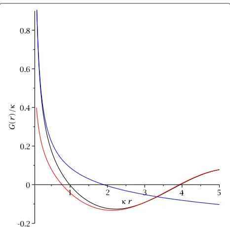
8[Y0(κr)+H0(κr)] , (25) whereH0(κr)is a Struve function. The Green’s function (25) has the property to approach a linear combination of two-dimensional and three-dimensional Green’s func-tions at small distances,

G(r) κr<0.5

1 4πr−

κ 4π

lnκr

2

+γ

, (26)

but it is very different from either the two-dimensional or three-dimensional behavior at large distances,

G(r)

κr>2.5 − κ 8πrsin

κr− π

4

(27)

(see Figure 2).

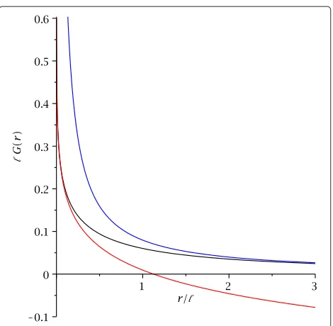
It is instructive to compare this to the Green’s function which results from different effective mass or different permittivity in a layer. The corresponding zero energy Green’s function [6]

G(r)= 1 8

H0 _r

−Y0 _r

(28)

yields two-dimensional behavior at small distancesr and three-dimensional behavior for large separation r,

r:G(r)= 1 4π

−γ−ln

_r

2

+r +O

r2 2

, (29)

r:G(r)= 1 4πr

1−

2

r2+O

4 r4

(30)

(see also Figure 3). Here, the length parameteris = am/m∗for an interface with different effective massm∗ for electrons or holes, or= a_∗/for an interface with different permittivity_∗.

To explore the question of two-dimensional or three-dimensional behavior in the quantum well further, we will look at the density of states in the quantum well.

Figure 3The zero energy Green’s function in a layer with different effective mass or permittivity.The blue line is the three-dimensional Green’s function(4πr)−1, the black line is the Green’s function (28) in a layer of different effective mass or different permittivity, and the red line is the two-dimensional logarithmic Green’s function·G= −[γ+ln(r/2)]/4π.

Density of states for the thin quantum well

The energy dependent retarded Green’s function is directly related to the density of states in a quantum system. This follows readily from the decomposition of (E−H+i)−1in terms of the spectrumEnand eigenstates |n,νofH,

G(E)= −2m

2G(E)= 1 E−H+i =

n,ν

|n,νn,ν| E−En+i

=P

n,ν

|n,νn,ν| E−En −

iπ

n,ν

δ(E−En)|n,νn,ν|.

(31)

Here, ν is a degeneracy index, and we tacitly imply that continuous components in the indices(n,ν)are inte-grated. We include spin in the set of quantum numbers (n,ν).

To make the connection with the density of states (or number of electronic orbitals) per volume, we observe that this quantity in general can be defined as

(E,x)= n,ν

δ(E−En)|x|n,ν|2. (32)

This implies the relation

(E,x)= −1

πx|G(E)|x. (33)

The quantum well atz0breaks translational invariance inzdirection, and we have with equation (33)

(E,z)= 4m

π2x,z|G(E)|x,z

= m

π32

d2kz|G(k,E)|z,

where a factorg = 2 was taken into account for spin 1/2 states.

If there is any quasi two-dimensional behavior in this system, we would expect it in the quantum well region. Therefore, we use the result (24) to calculate the density of states(E,z0)in the quantum well. Substitution yields

(E,z0) = m π32

d2kz0|G(k,E)|z0

= m

π

_∞

0

dk kδ2_k2_−2mE−κ

+ m

π2(E)

√

2mE/

0

dk k

√

2mE−2_k2 2mE−2_k2₊2_κ2, and after evaluation of the integrals,

(E,z0)=(2mE+2κ2)κ m π2

+(E) m

π23

√

2mE−κarctan

√

2mE κ

.

(34)

We can also express this in terms of the free two-dimensional and three-two-dimensional densities of electron states (cf. (13)),

(E,z0)=κd=2

E+(2κ2/2m)

+_d=3(E)

1−√κ

2mEarctan

_√

2mE κ

.

(35)

Note that K2 = E +(2κ2/2m) is the kinetic energy of the particles whose wave functions are exponentially suppressed perpendicular to the quantum well. We find that these particles indeed contribute a term proportional to the two-dimensional density of states _d=2(K2) with their energy K2 of motion along the quantum well, but with a dimensional proportionality constantκwhich is the inverse penetration depth of those states. Such a dimen-sional factor has to be there because densities of states in three dimensions enumerate states per energy and per volume, while_d=2(K2)counts states per energy and per area. Furthermore, the unbound states yield a contribu-tion which approaches the free three-dimensional density of states_d=3(E)in the limitκ→0.

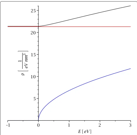
ranges in Figures 4 and 5. The density of states shows two-dimensional behavior for energies below the thresh-old where the electrons or holes can leave the quantum well and a linear combination of a two-dimensional term and three-dimensional term (with a correction factor) for energies above the threshold. This is again very differ-ent from the corresponding behavior of electrons or holes which move with different effective mass in a layer. In that case, the density of states in the layer approaches three-dimensional behavior for small separation and two-dimensional behavior for large separation [6] (see in par-ticular Equations (11) to (13) and Figure 1 in [6]).

Integration of (E,z0) yields the relation between the Fermi energy and the particle density in the quantum well. We find for−2κ2/2m ≤ EF ≤ 0 the two-dimensional area density for maximal kinetic energy K2,K = EF + (2κ2/2m)along the barrier, but rescaled with the inverse transverse penetration depth κ which converts it into a three-dimensional particle density,

n(z0)

−B<EF<0= κm π2

EF+

2_κ2

2m

=κn2 E2,F=K2,F

.

(36)

The result for EF > 0 is a combination of the scaled two-dimensional particle density (36) and the

three-Figure 4The density of states in the quantum well.This displays the density of states in the quantum well locationz₌z0for binding energyB₌1 eV, massm₌me=511 keV/c2, and energies −B_≤E_≤3 eV. The red curve is the contribution from states bound inside the quantum well, the blue curve is the pure three-dimensional density of states in absence of a quantum well, and the black curve is the density of states according to equation (34).

Figure 5The density of states (34) in the quantum well location

z=z0for higher energies0≤E≤100eV.The binding energy,

mass and color coding are the same as in Figure 4. The full density of states (34) approximates the three-dimensional√Ebehavior for energiesEB, but there remains a finite offset compared tod=3 due to the presence of the quantum well.

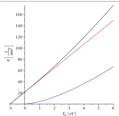
dimensional free particle densityn3with additional cor-rection terms,

n(z0) EF>0=

κ 2π22

×

κ2mEF−2κ2+2mEFarctan

√

2mEF

κ

+ κm

π2

EF+ 2_κ2

2m

+ 1

3π2

√

2mEF

3 ,

(37)

(see Figure 6).

The asymptotic form forEF 2κ2/2mis given by the three-dimensional densityn3plus sub-leading correction terms,

n(z0) EFB

1 3π2

√

2mEF

3

+ κm

2π2

EF+ 2_κ2

2m

+ κ2

π2

2mEF.

(38)

Figure 6The relation between particle density and Fermi energy.This displays the relation between particle density and Fermi energy in the quantum well for binding energyB=1 eV, mass

m=me=511 keV/c2, and−B≤EF≤6 eV. The red curve is the contribution from states bound inside the quantum well, the blue curve is the pure three-dimensional density of states in absence of a quantum well, and the black curve isn(EF)according to Equations (36) and (37).

that this is indeed a correct dimensionally hybrid Green’s function which yields inter-dimensional effects.

Not surprisingly, comparison of the relation between Fermi energy and density of fermions for the quantum well with the corresponding results for a layer of different effective mass [6] confirms again that the effective mass layer exhibits separation of two-dimensional behavior for small lengths/high energies and three-dimensional behav-ior for large lengths/small energies, whereas the quan-tum well yields a linear combination of two-dimensional and three-dimensional terms for small lengths/high energies.

Conclusions

The thin quantum well is certainly one of the most impor-tant model systems for low-dimensional structures in nano-science and technology. We have found that the Green’s function of this system resembles a linear combi-nation of two-dimensional and three-dimensional terms at small distances but exhibits oscillatory behavior at large distances. Furthermore, the local density of states and the relation between particle density and Fermi energy in the quantum well show two-dimensional behavior for Fermi energies below the threshold for scattering out

of the quantum well and a linear combination of two-dimensional and three-two-dimensional behavior plus correc-tion terms above the threshold. This behavior is very different from the behavior of charge carriers which move with different effective mass in a layer: in that case, the analysis in [6] had shown that the system exhibits two-dimensional behavior at small distances and high ener-gies, and three-dimensional behavior at large distances and low energies. The morale of the combination of the present results with the results of [6] is that if we wish to explicitly see transitions between two-dimensional and three-dimensional behavior in a system, then we should look for systems where the interface primarily affects the kinetic terms of fermions through a difference of effective mass between bulk and layer, or the kinetic terms of pho-tons through a difference of permittivity between bulk and layer.

Competing interests

The author declares that he has no competing interests.

Acknowledgements

This research was supported by NSERC Canada.

Received: 12 July 2012 Accepted: 3 October 2012 Published: 23 October 2012

References

1. Hayne M, Provoost R, Zundel MK, Manz YM, Eberl K, Moshchalkov VV:

Electron and hole confinement in stacked self-assembled InP quantum dots.Phys Rev B2000,62:10324–10328.

2. Albo A, Bahir G, Fekete D:Improved hole confinement in GaInAsN-GaAsSbN thin double-layer quantum-well structure for telecom-wavelength lasers.J Appl Phys2010,108:093116.

3. Nazir S, Upadhyay Kahaly M, Schwingenschl ¨ogl U:High mobility of the strongly confined hole gas in AgTaO3/SrTiO3.Appl Phys Lett2012,

100:201607.

4. Dick R:Hamiltonians and Green’s functions which interpolate between two and three dimensions.Int J Theor Phys2003,42:569–581. 5. Dick R:Dimensionally hybrid Green’s functions and density of states

for interfaces.Physica E2008,40:524–530.

6. Dick R:Dimensional effects on densities of states and interactions in nanostructures.Nanoscale Res Lett2010,5:1546–1554.

7. Dick R:Advanced Quantum Mechanics: Materials and Photons. New York: Springer; 2012.

8. Dick R:A model system for dimensional competition in

nanostructures: a quantum wire on a surface.Nanoscale Res Lett2008,

3:140–144.

9. Wang D, Zhao H, Wu N, El Khakani, M A, Ma D:Tuning the charge-transfer property of PbS-quantum dot/TiO2-nanobelt nanohybrids

via quantum confinement.J Phys Chem Lett2010,1:1030–1035. 10. Dick R:Dimensionally hybrid Green’s functions for impurity

scattering in the presence of interfaces.Physica E2008,40:2973–2976. 11. Ebert H, K ¨odderitzsch D, Min´ar J:Calculating condensed matter

properties using the KKR-Green’s function method—recent developments and applications.Rep Prog Phys2011,74:096501. 12. Abramowitz M, Stegun IA:Handbook of Mathematical Functions,9th

printing. New York: Dover Publications; 1970.

13. Kim KJ, Lee JC, Ahn SM, Lee KS, Lee CW, Cho YJ, Seo S, Shin KH, Choe SB, Lee HW:Interdimensional universality of dynamic interfaces.Nature

2009,458:740–742.

doi:10.1186/1556-276X-7-581

Cite this article as: Dick:Inter-dimensional effects in nano-structures.